The oscillation and stability of differentially rotating spherical shells: The initial-value problem

Abstract

An understanding of the oscillations of differentially rotating systems is key to many areas of astrophysics. It is of particular relevance to the emission of gravitational waves from oscillating neutron stars, which are expected to possess significant differential rotation immediately after birth or binary merger. In a previous paper we analysed the normal modes of a simple system exhibiting differential rotation. In this complementary paper we address the initial value problem for the same simple model using both analytical methods and numerical time evolutions. We derive a necessary and sufficient condition for dynamical shear instability. We discuss the dynamical behaviour of the continuous spectrum in response to an initial perturbation, and show that certain singular solutions within the continuous spectrum appear physically indistinguishable from the discrete modes outside the continuous spectrum.

1 Introduction

The oscillations of differentially rotating systems are important in many areas of astrophysics. They are of particular relevance to neutron star astrophysicists, because non-axisymmetric oscillations of compact stars are promising sources of gravitational waves. Detection and interpretation of gravitational waves from oscillating neutron stars could answer many questions about neutron star physics that are difficult to answer using electromagnetic observations, for example regarding the supranuclear equation of state. Emission of gravitational waves from neutron star oscillations will be strongest if the oscillations can grow via some dynamical or secular instability. The most promising instability scenarios arise for newly-born, accreting or newly-merged neutron stars. But it is in precisely these situations that we expect the stars to be differentially rotating. The latest simulations of core collapse indicate that the nascent neutron star emerges rotating differentially (Dimmelmeier, Font & Müller, 2002; Akiyama et al, 2003; Ott et al, 2004). Fujimoto (1993) has shown that rapid accretion from a companion could drive differential rotation in the surface layers of the neutron star, and a similar effect may occur during rapid accretion of supernova fallback material (Watts & Andersson, 2002). Shibata & Uryu (2000) and Baumgarte, Shapiro & Shibata (2000) have shown that a long-lived massive differentially rotating neutron star may be generated as the result of the merger of two neutron stars. In addition, recent work on r-modes in neutron stars suggests that the modes may drive a uniformly rotating star into differential rotation via non-linear effects (Rezzolla et al, 2000; Levin & Ushomirsky, 2001; Lindblom, Tohline & Vallisneri, 2001). Understanding the effect of differential rotation will be critical if we are to model gravitational wave emission from these systems correctly.

Differential rotation introduces two interesting phenomena. Firstly, it may lead to dynamical shear instabilities (Papaloizou & Pringle, 1984, 1985; Balbinski, 1985; Luyten, 1990). Secondly, the dynamical equations of the inviscid problem are complicated by the presence of corotation points. These are points where the pattern speed of a mode matches the local angular velocity, and at these points the governing equations are formally singular. The range of frequencies for which modes possess corotation points is termed the corotation band. It gives rise to a continuous spectrum, the dynamical role of which is unclear. Neither issue has received significant attention in the stellar perturbation literature (see Watts et al (2003), hereafter referred to as Paper I, for a summary of previous work).

We have begun to address the problem by modelling a simple system, a differentially rotating incompressible spherical shell. This model is simplistic, but exhibits the main features of the more complex three-dimensional problem. In Paper I we conducted a normal mode analysis for the shell. In the uniform rotation limit the shell problem admits only the standard r-modes as solutions. As the degree of differential rotation increases, the frequencies of these modes gradually approach the lower edge of the expanding corotation band. Most modes approach the boundary tangentially and appear to cease to exist when the degree of differential rotation exceeds a certain threshold value. In only a few cases do modes cross the corotation band boundary.

For real frequencies in the corotation band the shell problem admits a continuous spectrum of solutions with discontinuous first derivatives. In general, the continuous spectrum solutions have both a logarithmic singularity and a finite step in the first derivative at the corotation point. For certain special frequencies, however, the step in the first derivative vanishes. We refer to these solutions as zero-step solutions. Since these solutions appear when regular normal modes cross into the corotation band, they are likely to be of particular importance. Furthermore, in differentially rotating cylinders, these solutions can merge to give rise to dynamical instabilities (Balbinski, 1985). Even though we do not observe such behaviour in our problem it is an interesting possibility that should not be overlooked in future studies.

The character of the modes that cross into the corotation band varies. Only in one exceptional case, for the simplest rotation law examined, do we observe a mode crossing the corotation band boundary and continuing to exist as a regular stable mode. We think that such regular modes within the corotation band are unlikely to exist for more realistic rotation laws. In general, at all points where modes cross the corotation band boundary we observe the development of zero-step solutions. At some points we also observe the development of dynamically unstable modes. A necessary (but not sufficient) condition for dynamical instability is that the equilibrium vorticity have a turning point on the shell. Some of the rotation laws examined in Paper I meet this condition when the degree of differential rotation exceeds a certain threshold value. All modes crossing the corotation band boundary above this threshold become dynamically unstable. In addition, we observe for one rotation law the development of dynamical instability via the merger of two stable modes outside the corotation band.

Paper I raised a number of questions. Is it possible to derive a necessary and sufficient condition for instability? Do the singular solutions of the continuous spectrum have physical meaning? And do the zero-step solutions appear distinct from the continuous spectrum in time evolutions? In this paper we resolve these questions by addressing the initial value problem for the shell. By trying to isolate the various contributions to the evolution of smooth initial data, we hope to clarify the physical role of different parts of the spectrum of a differentially rotating system. The results for this simple toy model will guide us in future investigations of the three dimensional problem (Watts, Andersson & Jones, 2003).

2 Key results from the mode analysis

In Paper I we analysed the normal mode problem for the differentially rotating spherical shell. Since we will refer to a number of the results from the mode analysis in this paper, we summarise the key results in this section. Consider an incompressible fluid on a differentially rotating spherical shell (with radius $R$). Assuming that the perturbations are $\propto\exp(im\varphi)$ we have the $\theta$-component of the perturbed Euler equation,

$$\partial_{t}\delta v_{\theta}+im\Omega\delta v_{\theta}-2\Omega\cos\theta\delta v_{\varphi}=-\frac{1}{\rho R}\partial_{\theta}\delta P,$$ (1)

and the $\varphi$-component

$$\partial_{t}\delta v_{\varphi}+im\Omega\delta v_{\varphi}+\tilde{\Omega}\delta v_{\theta}=-\frac{im}{\rho R\sin\theta}\delta P,$$ (2)

where the equilibrium vorticity is

$$\tilde{\Omega}=2\Omega\cos\theta+\sin\theta\partial_{\theta}\Omega.$$ (3)

The perturbed continuity equation for an incompressible fluid is

$$\partial_{\theta}(\sin\theta\delta v_{\theta})+im\delta v_{\varphi}=0.$$ (4)

This tells us that only toroidal modes are permitted in this problem. Defining the stream function (in the standard way)

$$U=\delta v_{\theta}\sin\theta,$$ (5)

we can combine equations (1) and (2) to give the vorticity equation

$$(i\partial_{t}-m\Omega)\nabla_{\theta}^{2}U+\frac{m\partial_{\theta}\tilde{\Omega}}{\sin\theta}U=0,$$ (6)

where

$$\nabla^{2}_{\theta}=\partial_{\theta}^{2}+\frac{\cos\theta}{\sin\theta}\partial_{\theta}-\frac{m^{2}}{\sin^{2}\theta}$$ (7)

is the Laplacian on the unit sphere. Changing variables to $x=\cos\theta$ the vorticity equation becomes

$$(i\partial_{t}-m\Omega)\nabla^{2}_{x}U-m\tilde{\Omega}^{\prime}U=0,$$ (8)

where

$$\nabla^{2}_{x}=(1-x^{2})\partial_{x}^{2}-2x\partial_{x}-\frac{m^{2}}{1-x^{2}},$$ (9)

and we use a prime to denote derivatives with respect to $x$. In terms of $x$ the equilibrium vorticity is

$$\tilde{\Omega}=2x\Omega-(1-x^{2})\Omega^{\prime}.$$ (10)

Assuming that we are interested in a mode solution behaving as $\exp(-i\omega t)$, where $\omega$ is the frequency, equation (8) becomes

$$(\omega-m\Omega)\nabla^{2}_{x}U-m\tilde{\Omega}^{\prime}U=0.$$ (11)

At corotation points ($x=x_{c}$), $\omega=m\Omega(x_{c})$ and the equations are formally singular. The nature of the solutions in the vicinity of the corotation point can be analysed using the method of Frobenius. The general solution is found to be

$$U=U_{\mathrm{reg}}+U_{\mathrm{sing}},$$ (12)

where

$$U_{\mathrm{reg}}=\sum_{n=0}^{\infty}a_{n}(x-x_{c})^{n+1},$$ (13)

and

$$U_{\mathrm{sing}}=\sum_{n=0}^{\infty} \bigg{[} a_{n}(x-x_{c})^{n+1}\ln(x-x_{c}){}$$

$$+c_{n}(x-x_{c})^{n}\bigg{]}~{}~{}~{}~{}~{}~{}~{}~{}~{}~{}~{}~{}~{}~{}~{}~{}~{}x>x_{c}{}$$

$$U_{\mathrm{sing}}=\sum_{n=0}^{\infty} \bigg{[} b_{n}(x_{c}/x-1)^{n+1}\ln(x_{c}/x-1){}$$ (14)

$$+d_{n}(x_{c}/x-1)^{n}\bigg{]}~{}~{}~{}~{}~{}~{}~{}~{}~{}~{}~{}~{}~{}~{}x<x_{c}.$$

We use separate solutions for $U_{\mathrm{sing}}$ on either side of the corotation point to avoid taking the logarithm of a negative quantity. The two solutions for $U_{\mathrm{sing}}$ are matched such that $U$ is continuous at the corotation point. The first derivatives are however discontinuous at $x_{c}$, with (in general) both a logarithmic singularity and a step discontinuity. The size of this step discontinuity in $U^{\prime}$ varies as one traverses the frequency band spanned by the continuous spectrum, and for certain special frequencies it vanishes. We refer to the solutions at these frequencies as zero-step solutions. At the zero-step frequencies the Wronskian of the two linearly independent solutions to equation (11) vanishes, despite the logarithmic discontinuity in the first derivative. The importance of this will become apparent.

Let us now consider dynamical instabilities. From equation (8) it is possible to derive the necessary (but not sufficient) condition for instability $\tilde{\Omega}^{\prime}=0$. This condition is met for some of the rotation laws considered in Paper I when the degree of differential rotation exceeds some threshold value. Dynamical instabilities are then found to develop both where modes meet the corotation band boundary, and where modes merge outside the corotation band.

3 Evolving initial data: Green’s function approach

In this paper we consider equation (8) as an initial-value problem. That is, we are interested in the evolution of prescribed initial data, say,

$$U(x,t=0)=U_{0}(x).$$ (15)

We first transform the problem into the frequency domain via the Laplace transform (we use $s\to-i\omega$ in order to allow direct comparison with the mode calculations in Paper I).

$$\hat{U}=\int_{0}^{\infty}Ue^{i\omega t}dt,$$ (16)

with inverse

$$U=\frac{1}{2\pi}\int_{-\infty+ic}^{\infty+ic}\hat{U}e^{-i\omega t}d\omega.$$ (17)

Applying this transform to equation (8) we find

$$(\omega-m\Omega)\nabla^{2}_{x}\hat{U}-m\tilde{\Omega}^{\prime}\hat{U}=i\nabla^{2}_{x}U_{0}.$$ (18)

Note that $\nabla^{2}_{x}U_{0}$ is always non-zero for this problem. The only non-zero smooth initial data for which $\nabla^{2}_{x}U_{0}=0$ would violate the boundary conditions. We should also make a brief comment on the Laplace transform. For growing oscillatory $U$, with time dependence $\exp[(\alpha+i\beta)t]$, equation (18) is only correct if the imaginary part of $\omega$, $\omega_{I}$, is greater than $\alpha$. Otherwise the transform would fail to converge as $t\rightarrow\infty$. We must therefore ensure that the constant $c$, which appears in the limits of integration of the inverse Laplace transform in equation (17), lies above all of the poles of the integrand. This means that we must have $c>\alpha$. Thus on the line integral, we always have $\omega_{I}>\alpha$, and we never breach the assumption that we made when taking the Laplace transform. We then assume analytic continuation of the Laplace transform into the entire complex $\omega$ plane, and use the residue theorem to evaluate the line integral. This does not change the situation: the line integral itself always has $\omega_{I}>\alpha$ and the Laplace transform and its inverse are well-defined.

We will now use the Green’s function method to derive a formal solution to this equation (assuming for the moment that the problem is regular). Given a solution $G(\omega,x,y)$ to

$$\nabla^{2}_{x}G-\frac{m\tilde{\Omega}^{\prime}}{\omega-m\Omega}G=\delta(x-y),$$ (19)

we have

$$\hat{U}(\omega,x)=i\int_{0}^{1}\frac{G(\omega,x,y)}{\omega-m\Omega(y)}\nabla^{2}_{y}U_{0}(y)dy.$$ (20)

Note that because of the symmetry of the problem we need only consider the upper hemisphere of the shell. Finally, inverting the transform we obtain the solution to the initial value problem

$$U(x,t)=\frac{i}{2\pi}\int_{-\infty+ic}^{\infty+ic}d\omega~{}e^{-i\omega t}\int_{0}^{1}\frac{G(\omega,x,y)}{\omega-m\Omega(y)}\nabla^{2}_{y}U_{0}(y)dy.$$ (21)

The analytic properties of the integrand determine the spectrum of the problem.

In the standard way, we construct the required Green’s function $G(\omega,x,y)$ from solutions to the homogeneous problem. Thus we want to solve

$$(\omega-m\Omega)\nabla^{2}_{x}\hat{U}-m\tilde{\Omega}^{\prime}\hat{U}=0.$$ (22)

Consider two solutions, $\hat{U}_{L}$ and $\hat{U}_{R}$, that satisfy the boundary conditions at the left and right endpoints of the interval, respectively. Using the differential equation one can easily show that the Wronskian of any two solutions can be written

$$W=\hat{U}_{L}\hat{U}_{R}^{\prime}-\hat{U}_{R}\hat{U}_{L}^{\prime}=\frac{\tilde{W}(\omega)}{1-x^{2}}.$$ (23)

Pick an arbitrary point $y\in[0,1]$. Then an overall solution, that is continuous at $x=y$, can be written

$${\cal U}=C\left[H(x-y)\hat{U}_{L}(y)\hat{U}_{R}(x)+H(y-x)\hat{U}_{R}(y)\hat{U}_{L}(x)\right].$$ (24)

Working out the derivatives of this function, and using equation (22), we find that ${\cal U}$ is a solution to

$$\nabla^{2}_{x}{\cal U}-\frac{m\tilde{\Omega}^{\prime}}{\omega-m\Omega}{\cal U}=\delta(x-y)C\tilde{W}(\omega).$$ (25)

Comparing this to the equation for the Green’s function in the previous section we see that we can identify

$$G(\omega,x,y)=\frac{{\cal U}(\omega,x,y)}{C\tilde{W}(\omega)} = \frac{1}{\tilde{W}(\omega)}\Big{[}H(x-y)\hat{U}_{L}(y)\hat{U}_{R}(x){}$$ (26)

$$+H(y-x)\hat{U}_{R}(y)\hat{U}_{L}(x)\Big{]},$$

(clearly independent of the normalisation of $\hat{U}_{L}$ and $\hat{U}_{R}$).

4 Solving the initial value problem

To solve the initial value problem analytically we would need to evaluate the integrals:

$$U(x,t)=\frac{i}{2\pi}\int_{-\infty+ic}^{\infty+ic}\frac{{\cal J}(x,y)e^{-i\omega t}}{C\tilde{W}}d\omega$$ (27)

$${\cal J}(x,y)=\int_{0}^{1}\frac{{\cal U}(\omega,x,y)\nabla^{2}_{y}U_{0}(y)}{[\omega-m\Omega(y)]}dy,$$ (28)

where ${\cal U}$ is given by equation (24). Unfortunately, we cannot in general solve even the homogeneous problem (for $\hat{U}_{L}$ and $\hat{U}_{R}$) analytically. It is however possible to generate specific toy problems for which the initial value problem may be solved analytically. We are particularly interested in the behaviour of the continuous spectrum and the zero-step solutions. We therefore develop two toy problems. The first is a particular rotation law that admits only a continuous spectrum as a solution. An analytic solution of the initial value problem is possible for simple initial data, and the solution sheds light on the physical nature of the perturbation. In the second problem we aim to investigate the nature of the zero-step solutions. Ideally one would like to find a simple rotation law, with a zero-step solution, for which one could solve the initial value problem analytically. We have not been able to identify such a law. Instead we have developed a toy mathematical problem with solutions that include both a continuous spectrum and a zero-step solution. The behaviour of the eigenfunctions of this system near the critical point is mathematically identical to the behaviour that we find for the shell problem. The initial value problem for our toy system can however be solved analytically, guiding us towards a quasi-analytic solution for the zero-step solutions and continuous spectrum of the shell problem. The details of the two toy problems are contained in Appendices A and B. In this section we summarise only the key results from each problem.

Appendix A presents a full analytic solution of the initial value problem on the shell, for a simple rotation law that possesses only a continuous spectrum (with no zero-step solutions). For simple initial data the collective perturbation associated with the continuous spectrum is found to be non-singular, and hence physical. The perturbation dies away with time, with inverse power law decay rather than exponential decay. The frequency of the decaying perturbation depends in part upon position. Similar behaviour has been found for the continuous spectrum of a differentially rotating cylinder (Balbinski, 1984).

Appendix B introduces a toy problem that has singular continuous spectrum eigenfunctions with behaviour similar to those of our problem. By careful selection of boundary conditions, one can ensure the presence of a single zero-step solution within the continuous spectrum. In this case we are able to make some progress towards an analytic solution of the initial value problem. We draw several important conclusions that are likely to transfer to the differentially rotating shell. Firstly, the physical perturbation contains a constant amplitude oscillatory component at the zero-step frequency. Secondly, just as in Appendix A, the rest of the continuous spectrum dies away with time for simple initial data. Again we find inverse power law decay rather than exponential decay. The frequency of the perturbation associated with the continuous spectrum is, as before, found to depend in part upon position.

Let us now proceed as far as we can with the analytic solution to the initial value problem for the differentially rotating shell. We start by considering the integral over position, equation (28). We will write $\omega-m\Omega(y)\equiv\bar{\Omega}(\omega,y)(y-y_{c})$, where the corotation point $y_{c}$ is a function of $\omega$. Equation (28) becomes

$${\cal J}(x,y) = \hat{U}_{L}(x)\int_{x}^{1}\frac{\hat{U}_{R}(y)\nabla^{2}_{y}U_{0}(y)}{\bar{\Omega}(\omega,y)(y-y_{c})}dy{}$$ (29)

$$+\hat{U}_{R}(x)\int_{0}^{x}\frac{\hat{U}_{L}(y)\nabla^{2}_{y}U_{0}(y)}{\bar{\Omega}(\omega,y)(y-y_{c})}dy.$$

If $\omega$ is in the range of $m\Omega$, then $0<y_{c}<1$ and the integrand will be singular at $y=y_{c}$. In Paper I we examined the variation of $\hat{U}$ with $y$ and found that in the vicinity of the corotation point ($y\approx y_{c}$), for real $\omega$, it behaves as

$$\hat{U}=\sum_{n=0}^{\infty}c_{n}(y-y_{c})^{n}+\sum_{n=0}^{\infty}a_{n}(y-y_{c})^{n+1}\ln(y-y_{c}).$$ (30)

Whether $y_{c}$ is greater than or less than $x$ will depend on $\omega$. If $y_{c}>x$, the first integral in equation (29) has a pole and a branch point at $y=y_{c}$, and we must treat the integral as a principal value integral. If on the other hand $y_{c}<x$, then it is the second integral that must be treated as a principal value integral. The same procedure is followed in Appendix B. These integrals are not easily evaluated analytically; one must in general resort to numerical methods to solve even the homogeneous problem for $\hat{U}_{L}$ and $\hat{U}_{R}$. However, by examining the power series expansions around the singular point, which are identical to the power series expansions around the singular point for the problem in Appendix B, it is easy to see that the principal value integrals must result in smooth, non-singular functions. Thus even without solving the integrals analytically, we can state that the first integral will give rise to a function $I_{1}(x,\omega)$ and the second integral to a function $I_{2}(x,\omega)$, where both $I_{1}$ and $I_{2}$ are smooth, non-singular functions. The frequency integral, equation (27), becomes

$$U(x,t) = \frac{i}{2\pi}\int_{-\infty+ic}^{\infty+ic}\frac{1}{\tilde{W}(\omega)}\Big{[}\hat{U}_{L}(\omega,x)I_{1}(x,\omega){}$$ (31)

$$+\hat{U}_{R}(\omega,x)I_{2}(x,\omega)\Big{]}e^{-i\omega t}d\omega.$$

We cannot solve this integral analytically. Instead, we will use Cauchy’s theorem to extract its properties. We complete the contour using a semicircle of infinite radius in the lower half plane that must be deformed around any branch cuts. The contribution from the semicircle integral vanishes because the integrand tends to zero on this part of the contour. The only non-zero contribution will come from the poles and branch cuts of the integrand.

We know from Paper I that there are zeroes of $\tilde{W}$ at frequencies at which there are discrete normal modes, and at frequencies within the continuous spectrum where there are zero-step solutions. $\tilde{W}$ has a zero of multiplicity one in all cases except where modes or zero-step solutions merge: at these frequencies it has a zero of multiplicity two.

We must also consider the behaviour of $\hat{U}$. This function is well-behaved and non-singular except for $\omega$ within the range of $m\Omega$. Let us first consider the behaviour near the frequency $\omega=m\Omega(x)$, the corotation frequency. We need to know how $\hat{U}$ varies with $\omega$ for fixed $x$. This would in principle require a numerical calculation, but for the fact that we do know how $\hat{U}$ varies with $x$ for fixed $\omega$ in the vicinity of the point $x=x_{c}$. Because $x_{c}$ is a function of $\omega$, we can rewrite our power series expansions as an expansion around the singular frequency rather than the singular position (see Appendix B, where the equivalence is clearer). We find that $\hat{U}$ is non-singular but has a branch point at $\omega=m\Omega(x)$. The two end points of the continuous spectrum, $\omega=m\Omega_{\mathrm{min}}$ and $\omega=m\Omega_{\mathrm{max}}$ are also branch points. The contour of integration should look similar to that shown in Figure 4.

We can now make some definitive statements about the time-dependence of the physical perturbation $U(x,t)$.

1. The poles of the integrand at discrete frequencies $\omega_{n}$ where the Wronskian is zero will contribute terms with simple oscillatory time dependence $\exp(i\omega_{n}t)$. This is true both for discrete normal modes and the zero-step solutions. Thus by virtue of having zero Wronskian, the zero-step frequencies should appear virtually indistinguishable from the standard discrete normal modes, despite being in the continuous spectrum.

2. At frequencies where modes merge and the Wronskian has a double pole we will have additional terms of the form $t\exp(i\omega_{n}t)$. Such linear growth signals the onset of instability, as can be seen if one considers an unstable mode exhibiting exponential growth $\exp[(i\omega_{n}+\omega_{m})t]$. For small $\omega_{m}$ this can be expressed as a Taylor series:

   $$e^{i\omega_{n}t}e^{\omega_{m}t}\approx e^{i\omega_{n}t}\left[1+\omega_{m}t+\dots\right].$$ (32)

   This behaviour is to be expected since mode mergers usually lead to dynamical instability (Schutz, 1980).

3. The behaviour of the continuous spectrum is more difficult to ascertain but, since the end points of the corotation band on the real line are branch points, we would expect decaying oscillatory behaviour similar to that found in Appendix B. The frequency of oscillation will inevitably depend in part upon position. We cannot rule out the possibility of constant amplitude oscillation, or even growth of the continuous spectrum, in response to some initial data. What is clear, however, is that the perturbation associated with the continuous spectrum is non-singular and hence physical.

5 A sufficient instability condition

Having discussed the general properties of the solution, we will now use an analytic approach to the problem to derive a sufficient condition for instability. We follow the method outlined by Balmforth & Morrison (1999) for inviscid plane parallel shear flow. We start by reference to equation (25), the equation obeyed by ${\cal U}$. Let us assume that we can normalise the solution in such a way that

$$\int_{0}^{1}\nabla_{x}^{2}{\cal U}dx=\Lambda.$$ (33)

We assume that $\Lambda$ is real (note that, strictly speaking, $\Lambda$ will depend on $\omega$ and $y$). Then we find from equation (25) that

$$\Lambda=C\tilde{W}+\int_{0}^{1}\frac{m\tilde{\Omega}^{\prime}}{\omega-m\Omega}{\cal U}dx.$$ (34)

Hence

$$\epsilon\equiv C\tilde{W}=\Lambda-\int_{0}^{1}\frac{m\tilde{\Omega}^{\prime}}{\omega-m\Omega}{\cal U}dx.$$ (35)

In the limit when $\omega$ is real but outside the range $m\Omega(x_{c})$ for $x_{c}$ in [0,1], $\epsilon$ is real. $\epsilon$ has zeroes at frequencies where there are normal mode solutions outside the corotation band. If on the other hand $\omega$ is real, but in the range $\omega=m\Omega(x_{c})$ for $x_{c}\in[0,1]$, then the integrand is singular and the integral must be interpreted as the principal value.

$$\epsilon\equiv C\tilde{W} = \Lambda-{\cal P}\int_{0}^{1}\frac{m\tilde{\Omega}^{\prime}}{\omega-m\Omega}{\cal U}(\omega,x,y)dx{}$$ (36)

$$\pm i\pi\frac{\tilde{\Omega}^{\prime}(x_{c})}{\Omega^{\prime}(x_{c})}{\cal U}(\omega,x_{c},y).$$

The sign depends on whether we circle the singularity in the upper or the lower half-plane. This quantity $\epsilon$, as defined in equation (36), can be used to derive a sufficient instability criterion. Our next step is to derive a useful expression for ${\cal U}$.

In Section (3) we constructed a Green’s function for the initial value problem, equation (26), that depended on ${\cal U}$, which depends in turn on the solutions, $\hat{U}$, to the homogeneous problem. The equation for the homogeneous problem, equation (22) may be rewritten as

$$\nabla^{2}_{x}\hat{U}=\frac{m\tilde{\Omega}^{\prime}}{\omega-m\Omega}\hat{U}.$$ (37)

We can solve this equation using the Green’s function $G_{0}(x,x^{\prime})$ that satisfies

$$\nabla^{2}_{x}G_{0}=\delta(x-x^{\prime}).$$ (38)

The explicit form for this Green’s function is given in Appendix A. Finally, we have

$$\hat{U}(x)=\int_{0}^{1}\frac{m\tilde{\Omega}^{\prime}}{\omega-m\Omega}\hat{U}G_{0}(x,x^{\prime})dx^{\prime}.$$ (39)

Knowing that we can find $G_{0}$, we can rewrite equation (25) for ${\cal U}$ as an integral equation. We obtain

$${\cal U}(\omega,x,y) = C\tilde{W}G_{0}(x,y){}$$ (40)

$$+\int_{0}^{1}\frac{m\tilde{\Omega}^{\prime}}{\omega-m\Omega}{\cal U}(\omega,x^{\prime},y)G_{0}(x,x^{\prime})dx^{\prime},$$

or, if we use the normalisation, equation (33),

$${\cal U}(\omega,x,y) = \Lambda G_{0}(x,y)+\int_{0}^{1}\frac{m\tilde{\Omega}^{\prime}}{\omega-m\Omega}{\cal U}(\omega,x^{\prime},y){}$$ (41)

$$[G_{0}(x,x^{\prime})-G_{0}(x,y)]dx^{\prime}.$$

Recall that we have so far assumed that $\omega$ is complex in order to avoid singularities on the real $x$-axis. If we relax this assumption, we need to allow for the possibility that $\omega-m\Omega(x_{c})=0$. Then we find that (41) is a singular problem. However, we can regularise this equation by a judicious choice of $y$. We therefore take $y=x_{c}$ in (41) to get

$${\cal U}(\omega,x,x_{c}) = \Lambda G_{0}(x,x_{c})+\int_{0}^{1}\frac{m\tilde{\Omega}^{\prime}}{\omega-m\Omega}{\cal U}(\omega,x^{\prime},x_{c}){}$$ (42)

$$[G_{0}(x,x^{\prime})-G_{0}(x,x_{c})]dx^{\prime}.$$

As discussed by Balmforth & Morrison (1999), a solution to the Fredholm equation (42) is a singular eigenfunction associated with a continuous spectrum frequency. Note that we can let ${\cal U}(\omega,x,x_{c})\to{\cal U}(\omega,x)$ since $x_{c}$ is determined by $\omega$ anyway.

Equations (36) and (42) hold for all points where the normalisation given by equation (33) is valid. There are however certain solutions within the continuous spectrum for which this normalisation is not appropriate. If we have solutions for which $\tilde{W}=0$ then equation (25) for ${\cal U}$ is identical to the normal mode equation, (11), that we solved in Paper I. Thus for zero Wronskian solutions we can identify ${\cal U}$ with the normal mode solutions found in Paper I. Most zero Wronskian solutions correspond to modes with finite and continuous eigenfunctions outside the corotation band. The zero-step solutions are an exception, having zero Wronskian and a logarithmic discontinuity in the first derivative. So for the frequencies where zero-step solutions exist we must treat the integral in equation (33) as a principal value, with

$$\Lambda=\int_{0}^{1}\nabla_{x}^{2}{\cal U}dx={\cal P}\int_{0}^{1}\nabla_{x}^{2}{\cal U}dx\pm i\pi\left[(x-x_{c})\nabla_{x}^{2}{\cal U}\right]_{x=x_{c}}.$$ (43)

For these special frequencies,

$$\epsilon = {\cal P}\int_{0}^{1}\left[\nabla_{x}^{2}{\cal U}-\frac{m\tilde{\Omega}^{\prime}}{\omega-m\Omega}{\cal U}\right]dx{}$$ (44)

$$\pm i\pi\left[\left[(x-x_{c})\nabla_{x}^{2}{\cal U}\right]_{x_{c}}+\frac{\tilde{\Omega}^{\prime}(x_{c})}{\Omega^{\prime}(x_{c})}{\cal U}(\omega,x_{c},y)\right].$$

That the real part of $\epsilon$ should be zero if ${\cal U}$ is a solution to the normal mode problem is clear from equation (11). That the imaginary part must also be zero can be seen by taking the limit as $x\rightarrow x_{c}$ of $(x-x_{c})$ times equation (11), and applying L’Hôpital’s rule. So as we would expect, $\epsilon$ (and hence $\tilde{W}$) is zero at frequencies where there are zero-step solutions to the normal mode problem. For all other frequencies within the continuous spectrum $\epsilon$ will in general be complex and non-zero.

At frequencies where there are zero-step solutions, the regularising term in the integral in equation (42) cancels exactly the term involving $\Lambda$, and equation (42) becomes

$${\cal U}(\omega,x)=\int_{0}^{1}\frac{m\tilde{\Omega}^{\prime}}{\omega-m\Omega}{\cal U}(\omega,x^{\prime})G_{0}(x,x^{\prime})dx^{\prime}.$$ (45)

The equation becomes homogeneous, with a kernel that is truly singular. The presence of homogeneous solutions at certain frequencies complicates any attempts to solve equation (42) directly. Fortunately, we do not need to solve this equation to derive a sufficient instability criterion.

Let us recap. Given a solution to the integral equation (42), we can find the quantity $\epsilon$ defined in equation (36). These two equations hold for all frequencies in the continuous spectrum apart from those for which there are zero-step continuous spectrum solutions to the normal mode problem. At these frequencies, $\epsilon$ will be zero and there will be a homogeneous solution to equation (42), as discussed above.

Let us rescale equations (42) and (36) according to ${\cal U}/\Lambda\to{\cal U}$ and $\epsilon/\Lambda\to\epsilon$ to get

$${\cal U}(\omega,x) = G_{0}(x,x_{c})+\int_{0}^{1}\frac{m\tilde{\Omega}^{\prime}}{\omega-m\Omega}{\cal U}(\omega,x^{\prime}){}$$ (46)

$$[G_{0}(x,x^{\prime})-G_{0}(x,x_{c})]dx^{\prime},$$

and

$$\epsilon=1-{\cal P}\int_{0}^{1}\frac{m\tilde{\Omega}^{\prime}}{\omega-m\Omega}{\cal U}(\omega,x)dx\pm i\pi\frac{\tilde{\Omega}^{\prime}(x_{c})}{\Omega^{\prime}(x_{c})}{\cal U}(\omega,x_{c}).$$ (47)

In order to have an instability we must have a zero of the Wronskian $\tilde{W}$ in the upper half of the $\omega$-plane. The Nyquist method tells us that the number of zeroes ${\cal N}$ of $\tilde{W}$ in a region enclosed by a contour $\cal{C}$ in the $\omega$ plane is given by the integral

$${\cal N}=\frac{1}{2\pi i}\int_{\cal C}\frac{\tilde{W}^{\prime}}{\tilde{W}}d\omega=\frac{1}{2\pi}\Delta\mathrm{arg}(\tilde{W}),$$ (48)

where $\Delta$ is used to denote the change in a quantity. The integral in equation (48) tells us the number of times that the function $\tilde{W}$ winds around the origin of the complex $\tilde{W}$ plane as $\omega$ varies around $\cal C$. We decompose the integral into two parts:

$$\frac{1}{2\pi i}\int_{\cal{C}}\frac{\tilde{W}^{\prime}}{\tilde{W}}d\omega=\frac{1}{2\pi i}\int_{\cal{R}}\frac{\tilde{W}^{\prime}}{\tilde{W}}d\omega+\frac{1}{2\pi i}\int_{\cal{C}^{\prime}}\frac{\tilde{W}^{\prime}}{\tilde{W}}d\omega.$$ (49)

The first integral is taken over the real line $\cal{R}$, the second over a semicircle ${\cal C}^{\prime}$ in the upper half plane. In Appendix C we show that the integral over the semicircle vanishes. Now $\epsilon(\omega)=C(\omega)\tilde{W}(\omega)$, so

$$\int_{\cal R}\frac{\tilde{W}^{\prime}}{\tilde{W}}d\omega=\int_{\cal R}\frac{\epsilon^{\prime}}{\epsilon}d\omega-\int_{\cal R}\frac{C^{\prime}}{C}d\omega.$$ (50)

$C$ was an arbitrary constant in equation (24), so we can choose $C$ to be real. Then, setting $\epsilon=|\epsilon|\exp(i\mathrm{arg}\epsilon)$ and $\tilde{W}=|\tilde{W}|\exp(i\mathrm{arg}\tilde{W})$, equation (48) becomes

$${\cal N}=\frac{1}{2\pi}\Delta\mathrm{arg}(\epsilon).$$ (51)

In other words, the number of unstable eigenvalues should be determined by the change in the argument of $\epsilon$ as $\omega$ traverses the real line. In fact, we can constrain the range of integration still further. For frequencies outside the corotation band, the principal value integral in equation (47) becomes a regular integral with no imaginary part (since we can normalise ${\cal U}$ to ensure that it is real). Hence, $\epsilon$ is real for all frequencies outside the range $m\Omega_{\mathrm{min}}<\omega<m\Omega_{\mathrm{max}}$ and cannot wind. The presence of a corotation band and the associated continuous spectrum is clearly essential for instability on the shell. Thus

$${\cal N}=\frac{1}{2\pi}\Delta\mathrm{arg}(\epsilon)=\int_{m\Omega_{\mathrm{min}}}^{m\Omega_{\mathrm{max}}}\frac{\epsilon^{\prime}}{\epsilon}d\omega.$$ (52)

The existence of $\epsilon=0$ solutions at certain frequencies within the corotation band, and for certain degrees of differential rotation on the edges of the corotation band, will not affect the winding number. This is because these are isolated points where $\epsilon$ jumps directly to zero; and there is no winding if $\epsilon$ passes through the origin rather than around it. The frequencies where $\epsilon=0$ can be excluded from the calculation of winding number (Balmforth & Morrison, 1995), and will not be discussed further.

At the endpoints of the corotation band, $\omega=m\Omega_{\mathrm{min}}$ and $\omega=m\Omega_{\mathrm{max}}$, one can demonstrate that $\epsilon=1$. This means that there can only be winding if we cross the negative real $\epsilon$-axis while traversing the band.

From equation (47), it is clear that the imaginary part of $\epsilon$ is zero if either ${\cal U}(\omega,x_{c})=0$ or $\tilde{\Omega}^{\prime}(x_{c})=0$. The first condition, ${\cal U}(\omega,x_{c})=0$, cannot lead to instability, because if this is the case we have a regular mode within the corotation band, and the real part of $\epsilon$ would also vanish. Thus for winding we require

$$\tilde{\Omega}^{\prime}(x_{c})=0,$$ (53)

which is consistent with the necessary criterion for instability derived in Section 5. We denote the frequency at which this inflexion point condition is met as $\omega_{i}$.

For there to be at least one unstable eigenvalue, the real part of $\epsilon$ must be negative at the frequency $\omega_{i}$. We therefore have a sufficient condition for instability

$${\cal{P}}\int_{0}^{1}\frac{m\tilde{\Omega}^{\prime}}{\omega_{i}-m\Omega}{\cal U}(\omega_{i},x)dx>1.$$ (54)

The above condition tells us that there is at least one unstable eigenvalue. But what if we want to know the absolute number of unstable eigenvalues? In Paper I we found the total number of unstable eigenvalues by computing normal modes. The method outlined in this section offers in principle an alternative. If we could solve equation (46) numerically, using a Fredholm equation solving routine, we could use the resulting ${\cal U}$ to compute $\epsilon$ as the frequency varies across the continuous spectrum range, and hence determine the winding number directly. A similar calculation has been carried out by Balmforth & Morrison (1999) for plane parallel flow. Their problem is however simpler as there are no homogeneous solutions to their equivalent of equation (46). In our case one would have to begin by solving the homogeneous (eigenvalue) Fredholm problem, as stated in equation (45), and then exclude these frequencies from the main calculation. We have assessed the feasibility of solving the homogeneous equation using the numerical methods for singular integral equations discussed in Delves & Mohamed (1985), but conclude that application of these methods is far from trivial in this case. Computation of normal modes is a far more convenient method of determining the total number of unstable eigenvalues for this problem.

6 Evolving initial data: Numerical results

The prime way to check the mode calculations is the numerical evolution of generic smooth initial data. This will also enable us to check the quasi-analytic solution to the initial value problem formulated in Section 4.

We start by reformulating equation (6) to ensure that our variables are real valued. We introduce

$$U(t,\theta,\varphi)=C(t,\theta)\cos m\varphi-S(t,\theta)\sin m\varphi$$ (55)

After decoupling the sine/cosine parts, we arrive at two equations that can be written succinctly as

$$\partial_{t}A-m\Omega B+m\partial_{\theta}\tilde{\Omega}S = 0$$ (56)

$$\partial_{t}B+m\Omega A-m\partial_{\theta}\tilde{\Omega}C = 0$$ (57)

where $A$ and $B$ are defined by

$$\nabla^{2}_{\theta}C = \frac{A}{\sin\theta}$$ (58)

$$\nabla^{2}_{\theta}S = \frac{B}{\sin\theta}$$ (59)

In order to get a first-order system we introduce

$$Z = \partial_{\theta}C$$ (60)

$$X = \partial_{\theta}S$$ (61)

so equations (58) and (59) become

$$\sin\theta A-\sin^{2}\theta\partial_{\theta}Z-\sin\theta\cos\theta Z+m^{2}C = 0$$ (62)

$$\sin\theta B-\sin^{2}\theta\partial_{\theta}X-\sin\theta\cos\theta X+m^{2}S = 0$$ (63)

We now have six first order equations for six unknowns. We can see from equations (62)-(63) that for regularity at the poles we require $C=S=0$.

Our numerical solution of the six equations is based on a second order accurate Crank-Nicholson implicit finite differencing scheme. The finite differenced equations are solved using a relaxation scheme with $601$ gridpoints and a timestep $\Delta t=0.05\Delta\theta$. Convergence testing has verified that the code is second order accurate, and stability analysis indicates that the code is stable over many dynamical timescales. To test the code we ran time evolutions for the simple rotation law described in Appendix A. The analytical solution of the initial value problem was used to verify the robustness of the numerical time evolution code. We found the results to agree extremely well with those shown in Figure 3.

We then performed time evolutions for a more complicated rotation law, the solar rotation law that we studied in Paper I (Law 3 of that paper):

$$\Omega=2\pi\left(454.8-60.4\beta\cos^{2}\theta-71.4\beta\cos^{4}\theta\mathrm{~{}~{}nHz}\right)$$ (64)

The parameter $\beta$ measures the degree of differential rotation, uniform rotation corresponding to $\beta=0$.

For initial data we used the standard spherical harmonics $Y_{l}^{m}$ that are the eigenfunctions of $U$ in uniform rotation. A sample of numerical results for this rotation law with $m=2$ are shown in Figures 1-2. For frequencies outside the corotation band, there are clear peaks at the frequencies of the regular normal modes. For dynamically unstable modes we are able to verify the growth times predicted by the normal mode analysis. What is most interesting, however, is the behaviour of the continuous spectrum. The power spectrum shows distinct peaks within the continuous spectrum at frequencies where we found zero-step solutions in Paper I, just as predicted in Section 4. Although the size of the peak in the power spectrum varies depending on sampling position (the value of $x$ at which we monitor the time evolution), these frequencies clearly stand out from the rest of the continuous spectrum.

We were also interested to see how the rest of the continuous spectrum behaved in response to an initial perturbation. The continuous spectrum was observed to die away with time for smooth initial data, and to be excited to a much lower extent than the modes and zero-step solutions.

The numerical evolutions support the conclusions from our Green’s function analysis. In particular, it is clear that the zero-step solutions stand out from the rest of the continuous spectrum. Hence, it is reasonable to expect them to be of particular relevance for the dynamical evolution. This would be in accordance with the results of Balbinski (1985), which show that the merger of zero-step solutions may lead to dynamical instabilities.

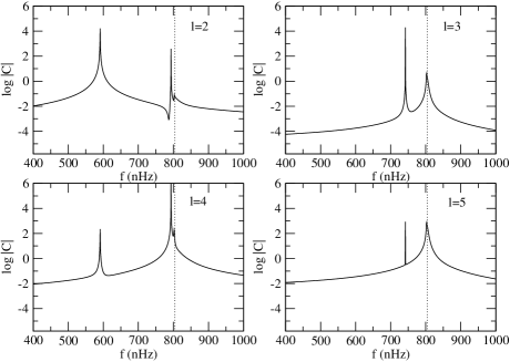
Figure 1: Power spectrum of numerical time evolution of data for the solar differential rotation law with $m=2$ and $\beta=0.4$. The four panels represent initial data proportional to the spherical harmonic $Y^{2}_{l}$, with $l=2-5$. The sampling position is $\theta=\pi/30$. The dashed line marks the lower edge of the corotation band, at 804.6. We know from Paper I that at $\beta=0.4$ the $l$ = 2, 3, and 4 modes are outside the corotation band, at frequencies 592.1, 744.3 and 796.0 respectively. Peaks at these frequencies are clearly visible. The $l=5$ mode does not cross into the corotation band but the mode results predict a zero-step solution just inside corotation, at frequency 806.35. A peak at this point is visible in the power spectrum.

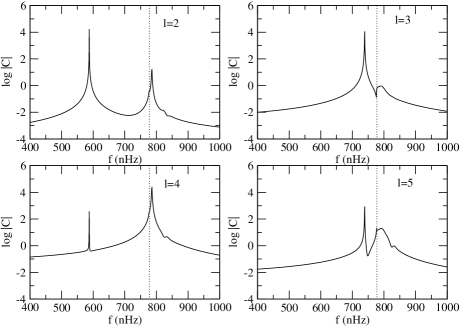
Figure 2: Power spectrum of numerical time evolution of data for the solar differential rotation law with $m=2$ and $\beta=0.5$. The four panels represent initial data proportional to the spherical harmonic $Y^{2}_{l}$, with $l=2-5$. The sampling position is $\theta=\pi/30$. The dashed line marks the lower edge of the corotation band, at 777.8. We know from Paper I that at $\beta=0.5$ the $l$ = 2 and 3 modes are outside the corotation band, at frequencies 588.66 and 741.08 respectively. Peaks at these frequencies are clearly visible. The $l$ = 4 mode is now inside the corotation band, at frequency 788.34. This is visible, in addition to a zero-step solution excited by $l=5$ initial data at 802.50. The peak at around 825 for $l$ = 4 and 5 initial data is probably associated with the continuous spectrum and is an artefact of sampling position.

7 Discussion

The main question arising from the normal mode analysis of Paper I was the nature of the physical perturbations associated with the singular eigenfunctions of both the zero-step corotating solutions, and the continuous spectrum within which they exist. By studying the initial value problem both analytically and numerically we have been able to resolve this issue.

Firstly, we have confirmed that the physical perturbations associated with these phenomena are not singular. Their time dependence in response to an initial perturbation, however, is complicated. For appropriate initial data, the zero-step solutions behave in much the same way as stable normal modes outside corotation. That is, they produce a clear peak in the power spectrum at a fixed frequency, standing out from the rest of the continuous spectrum. The fact that such oscillatory solutions can exist within the continuous spectrum is of great relevance for future studies of the oscillations of differentially rotating systems.

The behaviour of the rest of the continuous spectrum is difficult to predict analytically, and can only be elucidated by numerical time evolutions. The analytic calculations suggest that the physical perturbation associated with the continuous spectrum is oscillatory, with a complicated frequency dependence that varies in part according to the position on the shell. The amplitude of the oscillations could grow, remain at constant amplitude or die away with time (as a an inverse power of time), depending on the initial data and the rotation law. For the rotation laws and initial data that we have studied we observe only decay, but we cannot rule out either constant amplitudes or growth.

The results of numerical time evolutions have verified to high accuracy the predictions of mode frequencies made by the normal mode analysis. This is true both for modes outside the corotation band (including dynamically unstable modes), and the zero-step solutions within it. This is encouraging, as when we move on to study more realistic stellar models, we are likely to rely more on time evolutions than on increasingly complicated mode analysis.

8 Acknowledgments

We would like to thank Bernard Schutz and Horst Beyer for useful discussions. We acknowledge support from the EU Programme ‘Improving the Human Research Potential and the Socio-Economic Knowledge Base’ (Research Training Network Contract HPRN-CT-2000-00137). ALW is supported by a PPARC postgraduate studentship and NA acknowledges support from the Leverhulme Trust in the form of a prize fellowship.

Appendix A A rotation law that exhibits only a continuous spectrum

Solving the initial value problem analytically for an arbitrary rotation law is extremely difficult. For certain rotation laws, however, an analytical solution of the initial value problem is both feasible and instructive. In this Appendix we analyse a rotation law that exhibits a continuous spectrum but no other type of oscillation. Our aim is to isolate the response of the continuous spectrum to an initial perturbation. We select the simple rotation law

$$\Omega=\frac{\Omega_{c}}{1+|x|},$$ (65)

for which $\tilde{\Omega}^{\prime}=0$. Solving the normal mode problem for this rotation law, one finds that the only solutions form a continuous spectrum with derivatives that are discontinuous at the corotation point. In contrast to the general case, however, the derivatives possess only a step discontinuity at the corotation point (no logarithmic singularity). There are no zero-step solutions.

Returning to the initial value problem, equation (18) becomes

$$\nabla_{x}^{2}\hat{U}=\frac{i\nabla_{x}^{2}\hat{U}_{0}}{(\omega-m\Omega)}.$$ (66)

We solve this equation using a Green’s function $G_{0}(x,y)$ that satisfies

$$\nabla_{x}^{2}G_{0}=\delta(x-y).$$ (67)

Because of the symmetry of the governing equation there are two possible boundary conditions at $x=0$, either $dG_{0}/dx(0,y)=0$ (even solutions), or $G_{0}(0,y)=0$ (odd solutions). For even solutions, we find that

$$G_{0}(x,y)=\left\{\begin{array}[]{ll}\frac{-1}{2m}\left[\left(\frac{y+1}{y-1}\right)^{\frac{m}{2}}+\left(\frac{y-1}{y+1}\right)^{\frac{m}{2}}\right]\left(\frac{x-1}{x+1}\right)^{\frac{m}{2}}&x>y\\ \frac{-1}{2m}\left[\left(\frac{x+1}{x-1}\right)^{\frac{m}{2}}+\left(\frac{x-1}{x+1}\right)^{\frac{m}{2}}\right]\left(\frac{y-1}{y+1}\right)^{\frac{m}{2}}&x<y,\end{array}\right.$$ (68)

and for odd solutions,

$$G_{0}(x,y)=\left\{\begin{array}[]{ll}\frac{1}{2m}\left[\left(\frac{y-1}{y+1}\right)^{\frac{m}{2}}-\left(\frac{y+1}{y-1}\right)^{\frac{m}{2}}\right]\left(\frac{x-1}{x+1}\right)^{\frac{m}{2}}&x>y\\ \frac{1}{2m}\left[\left(\frac{x-1}{x+1}\right)^{\frac{m}{2}}-\left(\frac{x+1}{x-1}\right)^{\frac{m}{2}}\right]\left(\frac{y-1}{y+1}\right)^{\frac{m}{2}}&x<y.\end{array}\right.$$ (69)

We can now recover the physical perturbation using the inversion integral

$$U(x,t)=\int_{0}^{1}{\cal H}(x,y)\nabla^{2}_{y}U_{0}(y)dy,$$ (70)

where

$${\cal H}(x,y)=\frac{1}{2\pi}\int_{-\infty+ic}^{\infty+ic}\frac{G_{0}(\omega,x,y)e^{-i\omega t}}{\omega-m\Omega(y)}d\omega.$$ (71)

We illustrate the typical behaviour by giving results for the particular case $U_{0}(y)=P_{l}^{m}(y)$, with $l=m$ (even). In this case, $\nabla_{y}^{2}U_{0}(y)\propto(1-y^{2})^{m/2}$ and we find

$$U(x,t) = \frac{i(-1)^{m+1}}{4\pi m}\bigg{\{}\left(\frac{1-x}{1+x}\right)^{\frac{m}{2}}\int_{0}^{x}\Big{[}(1+y)^{m}+{}$$ (72)

$$(1-y)^{m}\Big{]}e^{-im\Omega(y)t}dy+\bigg{[}\left(\frac{1+x}{1-x}\right)^{\frac{m}{2}}+{}$$

$$\left(\frac{1-x}{1+x}\right)^{\frac{m}{2}}\bigg{]}\int_{x}^{1}(1-y)^{m}e^{-im\Omega(y)t}dy\bigg{\}}.$$

Evaluating the integral analytically for $l=m=1$ we find

$$U(x,t) = 2b\left[it\mathrm{Ei}(i\Omega_{c}t)-e^{-i\Omega_{c}t}\right]+\frac{(a+b)}{2}{}$$ (73)

$$\left[(4+2it)e^{-\frac{i\Omega_{c}t}{2}}+(t^{2}-4it)\mathrm{Ei}\left(\frac{i\Omega_{c}t}{2}\right)\right]{}$$

$$+\frac{1}{2}\Big{[}-3a+b+2(b-a)x-i(a+b)(1+x)t{}$$

$$+(a+b)x^{2}\Big{]}e^{-\frac{i\Omega_{c}t}{1+x}}+{}$$

$$\frac{1}{2}\left[4iat-(a+b)t^{2}\right]\mathrm{Ei}\left(\frac{i\Omega_{c}t}{1+x}\right),$$

where

$$a(x)=\left(\frac{1+x}{1-x}\right)^{\frac{1}{2}},~{}~{}b(x)=\left(\frac{1-x}{1+x}\right)^{\frac{1}{2}},$$ (74)

and the asymptotic expansion of the exponential integral $\mathrm{Ei}(x)$ is

$$\mathrm{Ei}(x)=\frac{e^{-x}}{x}\left(1-\frac{1}{x}+\frac{2}{x^{2}}-...\right).$$ (75)

Expanding the exponential integrals we find that all terms whose amplitudes grow with $t$ cancel. The resulting time dependence is illustrated in Figure 3. The most persistent term has an amplitude that decays as $1/t$. In addition, the three different frequency components $\Omega_{c}$, $\Omega_{c}/2$ and $\Omega_{c}/(1+x)$ interact to produce beating. The beating is particularly pronounced if $x$ is chosen such that $\Omega_{c}/(1+x)$ is very close to either of the other two frequencies.

If instead we consider initial data $U_{0}(y)=P_{l}^{m}(y)$ with $l=m+1$ (odd) then $\nabla_{y}^{2}U_{0}(y)\propto y(1-y^{2})^{m/2}$ and we find that

$$U(x,t) = \frac{i(-1)^{m}}{4\pi m}\bigg{\{}\left(\frac{1-x}{1+x}\right)^{\frac{m}{2}}\int_{0}^{x}y\Big{[}(1-y)^{m}-{}$$ (76)

$$(1+y)^{m}\Big{]}e^{-im\Omega(y)t}dy+\bigg{[}\left(\frac{1-x}{1+x}\right)^{\frac{m}{2}}-{}$$

$$\left(\frac{1+x}{1-x}\right)^{\frac{m}{2}}\bigg{]}\int_{x}^{1}y(1-y)^{m}e^{-im\Omega(y)t}dy\bigg{\}}.$$

Evaluating the integral analytically, we obtain similar results to those for $l=m$ initial data, except that now the most persistent terms decay as $1/t^{2}$. This is illustrated in Figure 3.

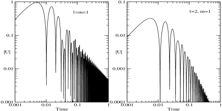
Figure 3: Time evolution of $|U|$ for $l=m=1$ and $l=2,m=1$ initial data. At late times, $|U|$ falls off as $1/t$ for the $l=m=1$ data and as $1/t^{2}$ for the $l=2,m=1$ data.

Appendix B A toy problem with a continuous spectrum and a zero-step solution

In Appendix A we solved the initial value problem for the differentially rotating shell for a rotation law that exhibits only a continuous spectrum. The continuous spectrum eigenfunctions obtained for this rotation law differ from those found for more general rotation laws, however, in two ways. Firstly, the eigenfunctions do not possess a logarithmic singularity in the first derivatives, only a finite step. Secondly, there are no zero-step solutions.

We have not been able to identify a rotation law that, in addition to exhibiting both of these features, is simple enough to permit analytical solution of the initial value problem. In this Appendix we instead analyse a toy problem that has solutions with the required behaviour, to inform our investigation of the shell problem.

B.1 Selection of a toy problem

Consider the equation

$$(x-i\partial_{t})U^{\prime\prime}(x)+U(x)=0,$$ (77)

where primes indicate derivatives with respect to $x$. Assume a normal mode solution, with $U\propto\exp(-i\omega t)$. Equation (77) becomes

$$(x-\omega)U^{\prime\prime}+U=0.$$ (78)

The critical point $x=\omega$, which gives rise to the continuous spectrum, plays the same role as the corotation point on the differentially rotating shell. The general solution to equation (78) is

$$U=\sqrt{x-\omega}[A_{1}J_{1}(2\sqrt{x-\omega})+A_{2}Y_{1}(2\sqrt{x-\omega})],$$ (79)

where $J_{\nu}$ and $Y_{\nu}$ are Bessel functions of the first and second kind respectively, $\nu$ being the index of the function. $A_{1}$ and $A_{2}$ are constants. To show that the solutions have the required behaviour, it is convenient to consider separate solutions on either side of the critical point (compare to Paper I):

$$U(x)=\left\{\begin{array}[]{ll}U_{<}(x)&x<\omega\\ U_{>}(x)&x>\omega,\end{array}\right.$$ (80)

where

$$U_{<}(x) = \sqrt{x-\omega}\left[c_{1}J_{1}(2\sqrt{x-\omega})+c_{2}Y_{1}(2\sqrt{x-\omega})\right]$$ (81)

$$U_{>}(x) = \sqrt{x-\omega}\left[c_{3}J_{1}(2\sqrt{x-\omega})+c_{4}Y_{1}(2\sqrt{x-\omega})\right]$$ (82)

where $c_{1}$ - $c_{4}$ are constants. Near the critical point:

$$U_{<} = -\frac{c_{2}}{\pi}+{\cal O}(x-\omega){}$$ (83)

$$U_{>} = -\frac{c_{4}}{\pi}+{\cal O}(x-\omega).$$ (84)

For continuity of the function at the critical point we require $c_{2}=c_{4}$. Let us now consider the behaviour of the first derivatives near the critical point:

$$U_{<}^{\prime} = c_{1}+\frac{c_{2}}{\pi}[\ln|x-\omega|+i\pi+2\gamma]+{\cal O}(x-\omega){}$$ (85)

$$U_{>}^{\prime} = c_{3}+\frac{c_{2}}{\pi}[\ln|x-\omega|+2\gamma]+{\cal O}(x-\omega),$$ (86)

where $\gamma$ is Euler’s constant. Thus at the critical point there will be both a logarithmic singularity and a finite step in the first derivative. The degree of freedom associated with the finite step in the first derivative allows us to construct a continuous spectrum of solutions for $\omega$ in the range of $x$. Mathematically the behaviour is identical to that of the continuous spectrum on the differentially rotating shell. The Wronskian of the two solutions, $W$, is

$$W=\frac{1}{\pi}[c_{4}c_{1}-c_{2}c_{3}+ic_{2}c_{4}].$$ (87)

Since $c_{2}=c_{4}$ we see that $W$ is zero if $c_{1}-c_{3}+ic_{2}=0$. This corresponds to the finite step in the first derivative vanishing, indicating the presence of a zero-step solution. As we are interested in the behaviour of zero-step solutions we will select a domain and boundary conditions such that there is at least one zero-step solution. We select the domain $x=[0,1]$ and fix one of the boundary conditions, $U_{<}(0)=0$. In this case there is a zero-step solution for $\omega=1/2$ if we insist on a second boundary condition $U_{>}(1)=\beta$, where

$$\beta=c_{3}\lim_{\omega\rightarrow 1/2}\left[\sqrt{1-\omega}\frac{[f_{2}f_{3}-f_{1}f_{4}+if_{1}f_{3}]}{f_{2}-if_{1}}\right],$$ (88)

and

$$f_{1}(\omega) = J_{1}(2\sqrt{-\omega}){}$$ (89)

$$f_{2}(\omega) = Y_{1}(2\sqrt{-\omega}){}$$ (90)

$$f_{3}(\omega) = J_{1}(2\sqrt{1-\omega}){}$$ (91)

$$f_{4}(\omega) = Y_{1}(2\sqrt{1-\omega}).$$ (92)

There are no other zero-step solutions within the continuous spectrum with $0<\omega<1$. Investigation suggests that there are no other mode solutions for this problem with these boundary conditions with either complex $\omega$ or real $\omega$ outside the range $0<\omega<1$.

B.2 Setting up the initial value problem

In the previous section we established the boundary conditions necessary to ensure that the toy problem exhibits both a continuous spectrum and a zero-step solution at $\omega=1/2$. We now define

$$\hat{U}=\int_{0}^{\infty}Ue^{-i\omega t}dt,$$ (93)

and apply a Laplace transform to equation (77) to obtain the inhomogeneous equation

$$\hat{U}^{\prime\prime}+\frac{\hat{U}}{x-\omega}=-\frac{iU_{0}^{\prime\prime}}{x-\omega}.$$ (94)

We will solve this problem using a Green’s function that obeys the equation

$$G^{\prime\prime}+\frac{G}{x-\omega}=\delta(x-y).$$ (95)

B.3 Finding the Green’s function

We construct the Green’s function as follows. Let $\hat{U}_{L}$ and $\hat{U}_{R}$ be solutions to the homogeneous equation that obey the boundary conditions on the left and right of the domain respectively. The Wronskian of these two solutions, $W$, is a function of frequency only. Consider the function

$$F(x,y)=C[H(y-x)\hat{U}_{R}(y)\hat{U}_{L}(x)+H(x-y)\hat{U}_{L}(y)\hat{U}_{R}(x)].$$ (96)

$F$ is continuous at the point $x=y$, irrespective of the normalisation of $\hat{U}_{L}$ and $\hat{U}_{R}$. It can be shown to obey the equation

$$F^{\prime\prime}+\frac{F}{x-\omega}=CW(\omega)\delta(x-y).$$ (97)

We can see that a valid solution to equation (95) is

$$G(\omega,x,y) = \frac{1}{W(\omega)}\Big{[}H(y-x)\hat{U}_{R}(y)\hat{U}_{L}(x){}$$ (98)

$$+H(x-y)\hat{U}_{L}(y)\hat{U}_{R}(x)\Big{]}.$$

We now need to determine $\hat{U}_{L}$ and $\hat{U}_{R}$. From our examination of the normal mode problem, we know that normalised solutions to the homogeneous problem are

$$\hat{U}_{L}(x)=\sqrt{x-\omega}\left[J_{1}(2\sqrt{x-\omega})+\bar{c}_{2}Y_{1}(2\sqrt{x-\omega})\right]$$ (99)

$$\hat{U}_{R}(x)=\sqrt{x-\omega}\left[J_{1}(2\sqrt{x-\omega})+\bar{c}_{4}Y_{1}(2\sqrt{x-\omega})\right],$$ (100)

where (comparing to the normal mode problem) we have defined $\bar{c}_{2}=c_{2}/c_{1}$, $\bar{c}_{4}=c_{4}/c_{3}$, and $\bar{\beta}=\beta/c_{3}$. The Wronskian of the two solutions is

$$W=\bar{c}_{4}-\bar{c}_{2}+i\bar{c}_{2}\bar{c}_{4}.$$ (101)

The boundary condition at $x=0$, $\hat{U}_{L}(0)=0$, gives

$$\bar{c}_{2}=-\frac{J_{1}(2\sqrt{-\omega})}{Y_{1}(2\sqrt{-\omega})}.$$ (102)

The boundary condition at $x=1$, $\hat{U}_{R}(1)=\bar{\beta}$, gives

$$\bar{c}_{4}=\frac{1}{Y_{1}(2\sqrt{1-\omega})}\left[\frac{\bar{\beta}}{\sqrt{1-\omega}}-J_{1}(2\sqrt{1-\omega})\right].$$ (103)

It can be verified that the Wronskian is indeed zero at $\omega=1/2$. We have now found our Green’s function.

B.4 The inversion integrals (part I)

The first stage in recovering $U(x,t)$ is to use the Green’s function to find $\hat{U}(x,\omega)$. Using equations (94) and (95) we can show, in the standard way, that

$$\hat{U}(x)=-i\int_{0}^{1}\frac{U_{0}^{\prime\prime}G}{y-\omega}dy-\left[G\hat{U}^{\prime}-\hat{U}G^{\prime}\right]_{0}^{1}.$$ (104)

The last term in equation (104) is non-zero because of our choice of boundary conditions. By choosing conditions that ensured the presence of a zero-step solution, we have also ensured that $G$ and $\hat{U}$ do not obey the same boundary conditions. In the following sections we will neglect this second term because our primary interest is in the zero-step solutions. Their contribution is encapsulated in the position integral, not in the second term, which depends solely on the end-points. Restricting our attention to the position integral,

$$\int_{0}^{1}\frac{U_{0}^{\prime\prime}(y)G(\omega,x,y)}{y-\omega}dy = \frac{1}{W(\omega)}\Big{[}\hat{U}_{L}(x)\left(I_{p1}+\bar{c}_{4}(\omega)I_{p2}\right){}$$ (105)

$$+\hat{U}_{R}(x)\left(I_{p3}+\bar{c}_{2}(\omega)I_{p4}\right)\Big{]}$$

where

$$I_{p1} = \int_{x}^{1}\frac{J_{1}(2\sqrt{y-\omega})}{\sqrt{y-\omega}}dy{}$$ (106)

$$I_{p2} = \int_{x}^{1}\frac{Y_{1}(2\sqrt{y-\omega})}{\sqrt{y-\omega}}dy{}$$ (107)

$$I_{p3} = \int_{0}^{x}\frac{J_{1}(2\sqrt{y-\omega})}{\sqrt{y-\omega}}dy{}$$ (108)

$$I_{p4} = \int_{0}^{x}\frac{Y_{1}(2\sqrt{y-\omega})}{\sqrt{y-\omega}}dy.$$ (109)

In order to evaluate these integrals we must select initial data that obeys the boundary conditions. We will consider the simple case

$$U_{0}(y)=y^{2}/2+(\bar{\beta}-1/2)y~{}~{}\rightarrow~{}~{}U_{0}^{\prime\prime}=1.$$ (110)

$I_{p1}$ and $I_{p3}$ are regular at the point $y=\omega$, so the integrals are straightforward:

$$I_{p1}=J_{0}(2\sqrt{x-\omega})-J_{0}(2\sqrt{1-\omega}),$$ (111)

$$I_{p3}=-J_{0}(2\sqrt{x-\omega})+J_{0}(2\sqrt{-\omega}).$$ (112)

The integrals $I_{p2}$ and $I_{p4}$ require a little more care because the integrands are singular at the point $y=\omega$ (real $\omega$ only). If $x<\omega<1$, we must treat $I_{p2}$ as a principal value integral, and $I_{p4}$ is non-singular. If on the other hand $0<\omega<x$, we must treat $I_{p4}$ as a principal value integral, and $I_{p2}$ is non-singular. Thus we get

$$I_{p2}=Y_{0}(2\sqrt{x-\omega})-Y_{0}(2\sqrt{1-\omega})-H(\omega-x)i,$$ (113)

$$I_{p4}=-Y_{0}(2\sqrt{x-\omega})+Y_{0}(2\sqrt{-\omega})-H(x-\omega)i.$$ (114)

B.5 The inversion integrals (part II)

The final inversion integral to recover the time dependent solution $U(x,t)$ is

$$U(x,t)=\frac{1}{2\pi}\int_{-\infty+ic}^{\infty+ic}\hat{U}(\omega,x)e^{-i\omega t}d\omega.$$ (115)

For our given choice of initial data, equation (115) becomes:

$$U(x,t) = \frac{1}{2\pi}\int_{-\infty+ic}^{\infty+ic}\frac{e^{-i\omega t}\sqrt{x-\omega}}{W(\omega)}\Big{\{}J_{1}(2\sqrt{x-\omega}){}$$ (116)

$$\left[J_{0}(2\sqrt{-\omega})-J_{0}(2\sqrt{1-\omega})\right]+J_{1}(2\sqrt{x-\omega}){}$$

$$\big{[}(\bar{c}_{4}-\bar{c}_{2})Y_{0}(2\sqrt{x-\omega})-\bar{c}_{4}Y_{0}(2\sqrt{1-\omega})+{}$$

$$\bar{c}_{2}Y_{0}(2\sqrt{-\omega})\big{]}+Y_{1}(2\sqrt{x-\omega})\big{[}(\bar{c}_{2}-\bar{c}_{4}){}$$

$$J_{0}(2\sqrt{x-\omega})+\bar{c}_{4}J_{0}(2\sqrt{-\omega})-\bar{c}_{2}J_{0}(2\sqrt{1-\omega})\big{]}{}$$

$$-i\bar{c}_{2}\bar{c}_{4}Y_{1}(2\sqrt{x-\omega})-iJ_{1}(2\sqrt{x-\omega}){}$$

$$\left[H(\omega-x)\bar{c}_{4}+H(x-\omega)\bar{c}_{2}\right]\Big{\}}.$$

The integrand has a simple pole at $\omega=1/2$ due to the zero of the Wronskian. In addition, there are branch points at $\omega=0,x,1$. The contour of integration for $x<1/2$ is shown in Figure 4 (if $x>1/2$, we would instead join the points $\omega=x$ and $\omega=1$ by a branch cut, and have an isolated branch cut down from $x=0$). The integral around the semicircle, I2, vanishes as the radius tends to infinity, while the integrals along I5/I6 and I7/I10 cancel exactly.

Figure 4: The contour for the frequency inversion integral. Filled dots indicate branch points, open dots isolated poles. The thick solid lines are branch cuts.

The residue associated with the simple pole at $\omega=1/2$ is $\propto\exp(-it/2)$. Such constant amplitude oscillatory frequency contributions are typical of frequencies where there are zero-step solutions. Identical behaviour is found for the shell model, as discussed in Section 4.

Working out the contributions from I3, I4, I8 and I9 is more difficult. We will focus on I8/I9, as the continuous spectrum contribution arises from the branch point at $\omega=x$. We restrict our attention to the case when $x$ is small (for illustrative purposes). Making this assumption we note that $\omega$ and $\omega-x$ are also small on I8 and I9. We will use Taylor expansions of the integrand using the three small parameters $x$, $\omega$, and $\omega-x$ .

Keeping only terms up to second order, we find that the contribution to equation (116) from the integrals along I8 and I9, $I_{\omega}$, is

$$I_{\omega} = \int_{I8,I9}e^{-i\omega t}(W_{0}+W_{1}\omega)\Big{[}\alpha_{1}(x-\omega)\ln(x-\omega){}$$ (117)

$$+\alpha_{2}(x-\omega)^{2}\ln(x-\omega)+\alpha_{3}\omega(x-\omega)\ln(x-\omega){}$$

$$+\alpha_{4}\omega^{2}\ln(-\omega)+\alpha_{5}\omega(x-\omega)\ln(-\omega)\Big{]},$$

where $\alpha_{1}$ - $\alpha_{5}$ are constants, and we have expanded the inverse Wronskian in terms of the small parameter $\omega$:

$$W(\omega)^{-1}=W_{0}+W_{1}\omega+{\cal O}(\omega^{2}),$$ (118)

where $W_{0}$ and $W_{1}$ are also constants. We now choose the phase of the logarithms such that

$$\ln(-\omega)=\left\{\begin{array}[]{ll}\ln|\omega|&\mathrm{~{}~{}~{}~{}On~{}I8}\\ \ln|\omega|+2\pi i&\mathrm{~{}~{}~{}~{}On~{}I9}\end{array}\right.$$ (119)

$$\ln(x-\omega)=\left\{\begin{array}[]{ll}\ln|x-\omega|&\mathrm{~{}~{}~{}~{}On~{}I8}\\ \ln|x-\omega|+2\pi i&\mathrm{~{}~{}~{}~{}On~{}I9.}\end{array}\right.$$ (120)

The logarithm terms cancel when we integrate over I8 and I9, so the only non-zero contribution will come from the $2\pi i$ piece on I9. At first order, the contribution to $I_{\omega}$ is

$$I_{\omega 1}=\beta_{1}\left[\frac{1-ixt-e^{-ixt}}{t^{2}}\right],$$ (121)

where $\beta_{1}$ is a constant. The second order contribution to $I_{\omega}$ is

$$I_{\omega 2}=\frac{1}{t^{3}}\left[\gamma_{1}+\gamma_{2}xt+\gamma_{3}x^{2}t^{2}+\left(\delta_{1}+\delta_{2}xt+\delta_{3}x^{2}t^{2}\right)e^{-ixt}\right],$$ (122)

where $\gamma_{1}-\gamma_{3}$ and $\delta_{1}-\delta_{3}$ are constants. If we include higher order terms we find that that the most persistent contribution to $U(x,t)$ arising from the continuous spectrum decays as $1/t$. Higher order terms merely introduce contributions that decay as successively higher order powers of $t$. It is also clear that the continuous spectrum contributes a term to $U(x,t)$ with a frequency that depends on position $x$.

The analysis presented in this section is for a specific choice of initial data and for small $x$. We must therefore ask whether the key results would change if we had made different choices. It is certainly by no means clear that the continuous spectrum should decay for all smooth initial data. Although we have not observed anything other than decay, we cannot rule out the possibility of constant amplitude oscillation or even growth. In contrast, the existence of a frequency component that depends on position appears inevitable.

Appendix C Vanishing of semicircle integral in derivation of instability criterion

In this Appendix we will demonstrate that we can neglect the integral over the semicircle in equation (49) by considering the nature of solutions for large $|\omega|$. We start by rewriting equation (22) as

$$\nabla^{2}_{x}\hat{U}-\frac{m}{\omega}\left[\Omega\nabla^{2}_{x}\hat{U}-\tilde{\Omega}^{\prime}\hat{U}\right]=0.$$ (123)

We expand $\hat{U}$ in terms of the small parameter $m/\omega$

$$\hat{U}=\hat{U}_{0}+\frac{m}{\omega}\hat{U}_{1}.$$ (124)

Equation (123) becomes

$$\nabla^{2}_{x}\hat{U}_{0}+\frac{m}{\omega}\nabla^{2}_{x}\hat{U}_{1}-\frac{m}{\omega}\Big{[}\Omega\nabla^{2}_{x}\hat{U}_{0}+\frac{m}{\omega}\Omega\nabla^{2}_{x}\hat{U}_{1}$$

$$-\tilde{\Omega}^{\prime}\hat{U}_{0}-\frac{m}{\omega}\tilde{\Omega}^{\prime}\hat{U}_{1}\Big{]} = 0.$$ (125)

At leading order equation (125) becomes

$$\nabla^{2}_{x}\hat{U}_{0}=0.$$ (126)

At first order equation (125) becomes

$$\nabla^{2}_{x}\hat{U}_{1}+\tilde{\Omega}^{\prime}\hat{U}_{0}=0.$$ (127)

The general solution to equation (126) is

$$\hat{U}_{0}=\left\{\begin{array}[]{llll}\hat{U}_{0R}&=&c_{1}\left(\frac{x-1}{x+1}\right)^{\frac{m}{2}}&x>y\\ \hat{U}_{0L}&=&c_{2}\left(\frac{x+1}{x-1}\right)^{\frac{m}{2}}+c_{3}\left(\frac{x-1}{x+1}\right)^{\frac{m}{2}}&x<y,\end{array}\right.$$ (128)

where for continuity of the function at $x=y$ we require

$$c_{1}=c_{2}\left(\frac{y+1}{y-1}\right)^{m}+c_{3}.$$ (129)

It is clear from equation (128) that $\hat{U}_{0}$ does not depend on $\omega$. Using the method of Green’s functions to solve equation (127) we must first solve

$$\nabla_{x}^{2}G_{0}=\delta(x-x^{\prime}).$$ (130)

The solution to this equation is given in Appendix A, equations (68) and (69). We find $G_{0}(x,x^{\prime})$ to be independent of $\omega$. We now have

$$\hat{U}_{1}=\left\{\begin{array}[]{lll}\hat{U}_{1R}=-\int G_{0}(x,x^{\prime})\tilde{\Omega}^{\prime}(x^{\prime})\hat{U}_{0R}(x^{\prime},y)dx^{\prime}&x>y\\ \hat{U}_{1L}=-\int G_{0}(x,x^{\prime})\tilde{\Omega}^{\prime}(x^{\prime})\hat{U}_{0L}(x^{\prime},y)dx^{\prime}&x<y.\end{array}\right.$$ (131)

It is clear from equation (131) that $\hat{U}_{1}$ must also be independent of $\omega$. Let us consider the implications of this for the Wronskian $W$. We get

$$W = \hat{U}_{0L}\hat{U}_{0R}^{\prime}-\hat{U}_{0R}\hat{U}_{0L}^{\prime}+\frac{m}{\omega}\Big{[}\hat{U}_{1L}\hat{U}_{0R}^{\prime}-\hat{U}_{0R}\hat{U}_{1L}^{\prime}{}$$ (132)

$$+\hat{U}_{0L}\hat{U}_{1R}^{\prime}-\hat{U}_{1R}\hat{U}_{0L}^{\prime}\Big{]}+\sim{\cal O}\left(\frac{m}{\omega}\right)^{2}.$$

This means that we can write $\tilde{W}=(1-x^{2})W$ as

$$\tilde{W}=f(x,y)+\frac{m}{\omega}g(x,y),$$ (133)

and we obtain

$$\frac{\tilde{W}^{\prime}}{\tilde{W}}=-\frac{mg(x,y)/\omega^{2}}{f(x,y)+mg(x,y)/\omega}\approx-\frac{mg(x,y)f(x,y)}{\omega^{2}}.$$ (134)

Integrating over frequency,

$$\int_{{\cal C}^{\prime}}\frac{\tilde{W}^{\prime}}{\tilde{W}}d\omega=-\frac{mg(x,y)f(x,y)}{\omega}.$$ (135)

In the limit as $\omega\rightarrow\infty$ the integral clearly tends to zero. We can therefore neglect the integral over the infinite semicircle in equation (49).

References

- Akiyama et al (2003) Akiyama S., Wheeler J.C., Meier D.L., Lichtenstadt I., 2003, ApJ, 584, 954
- Balbinski (1984) Balbinski E., 1984, MNRAS, 209, 145
- Balbinski (1985) Balbinski E., 1985, MNRAS, 216, 897
- Balmforth & Morrison (1995) Balmforth N.J., Morrison P.J., 1995, Annals New York Academy of Sciences, 773, 80
- Balmforth & Morrison (1999) Balmforth N.J., Morrison P.J., Studies in Applied Math., 102, 309
- Baumgarte, Shapiro & Shibata (2000) Baumgarte T.W., Shapiro S.L., Shibata M., 2000, ApJ, 528, L29
- Delves & Mohamed (1985) Delves L.M., Mohamed J.L., 1985, Computational methods for integral equations, Cambridge Univ. Press, Cambridge
- Dimmelmeier, Font & Müller (2002) Dimmelmeier H., Font J.A., Müller E., 2002,A&A, 388, 917
- Friedman & Schutz (1978a) Friedman J.L., Schutz B.F., 1978, ApJ, 221, 937
- Fujimoto (1993) Fujimoto M.Y., 1993, ApJ, 419, 768
- Levin & Ushomirsky (2001) Levin Y., Ushomirsky G., 2001, MNRAS, 322, 515
- Lindblom, Tohline & Vallisneri (2001) Lindblom L., Tohline J.E., Vallisneri M., 2001, Phys. Rev. Lett., 86, 1152
- Luyten (1990) Luyten P.J., 1990, MNRAS, 242, 447
- Ott et al (2004) Ott C.D., Burrows A., Livne E., Walder R., 2004, ApJ, 600, 834
- Papaloizou & Pringle (1984) Papaloizou J.C.B., Pringle J.E., 1984, MNRAS, 208, 721
- Papaloizou & Pringle (1985) Papaloizou J.C.B., Pringle J.E., 1985, MNRAS, 213, 799
- Rezzolla et al (2000) Rezzolla L., Lamb F.L., Shapiro S.L., 2000, ApJ, 531, L139
- Schutz (1980) Schutz B.F., 1980, MNRAS, 190, 7
- Shibata & Uryu (2000) Shibata M., Uryu K., 2000, Phys. Rev. D, 61, 064001
- Watts & Andersson (2002) Watts A.L., Andersson N., 2002, MNRAS, 333, 943
- Watts et al (2003) Watts A.L., Andersson N., Beyer H., Schutz B.F., 2003, MNRAS, 342, 1156
- Watts, Andersson & Jones (2003) Watts A.L., Andersson N., Jones D.I., 2003, astro-ph/0309554