Cosmic microwave background anisotropies in multi-connected flat spaces

Abstract

This article investigates the signature of the seventeen multi-connected flat spaces in cosmic microwave background (CMB) maps. For each such space it recalls a fundamental domain and a set of generating matrices, and then goes on to find an orthonormal basis for the set of eigenmodes of the Laplace operator on that space. The basis eigenmodes are expressed as linear combinations of eigenmodes of the simply connected Euclidean space. A preceding work, which provides a general method for implementing multi-connected topologies in standard CMB codes, is then applied to simulate CMB maps and angular power spectra for each space. Unlike in the 3-torus, the results in most multi-connected flat spaces depend on the location of the observer. This effect is discussed in detail. In particular, it is shown that the correlated circles on a CMB map are generically not back-to-back, so that negative search of back-to-back circles in the WMAP data does not exclude a vast majority of flat or nearly flat topologies.

I Introduction

Among all multi-connected three-dimensional spaces, “flat spaces” have been studied the most extensively in the cosmological context. This is due to the computational simplicity of the simplest compact flat three-manifold, the 3-torus, which has been used extensively in numerical simulations. The main goal of this article is to provide tools to compute the CMB properties and produce high resolution CMB maps for all seventeen multi-connected flat spaces , following the general method introduced in our preceding work [1].

Recent measurements show that the density parameter $\Omega_{0}$ is close to unity and the observable universe is approximately flat. CMB data obtained by the Archeops balloon experiments [2] and more recently by WMAP [3] place strong constraints on the curvature. In addition, WMAP [4] and later the Planck satellite [5] do and will provide full sky maps of CMB anisotropies, offering an opportunity to probe the topological properties of our universe. This observational constraint on the curvature radius of the universe motivates the detailed study of flat spaces even though spherical spaces are also promising candidates [6, 7, 8, 9, 10, 11].

At present, the status of the constraints on the topology of flat spaces is evolving rapidly driven by the release of the WMAP data. Previous analysis, based on the COBE data, mainly constrained the topology of a 3-torus (see Refs. [12, 13, 14, 15, 16, 17, 18, 19, 20, 21, 22] and Refs. [23, 24, 25] for reviews of different methods for searching for the topology).

The WMAP data [3] possess some anomalies on large angular scales that may be explained by a topological structure. In particular, the quadrupole is abnormally low, the octopole is very planar and the alignment between the quadrupole and octopole is also anomalous [26]. Besides many other potential explanations [27], it was suggested that a toroidal universe with a smaller dimension on the order of half the horizon scale may explain all these anomalies [26] but it was latter shown, on the basis of a finer statistical analysis, that it did not [28]. Another topology was recently proposed to explain some of this anomaly in the case of a slightly positively curved space, namely the Poincaré dodecahedral space [11].

The first results of the search for the topology through the “circles in the sky” method [29] gave negative results for back-to-back or almost back-to-back circles [28, 30]. While the first applies only to back-to-back circle with no twist, the second study includes an arbitrary twist and conclude that “it rules out the possibility that we live in a universe with topology smaller than $24\,{\mbox{Gpc}}$”. As will be discussed in this paper, back-to-back circles are generic only for homogeneous topologies such as e.g. 3-tori and a subclass of lens spaces. In non-homogeneous spaces the relative position of the circles depends on the position of the observer in the fundamental polyhedron.

In conclusion, as demonstrated by these preliminary results, only the toroidal spaces have been really constrained [28, 30]. Besides, a series of studies have pointed out a departure of the WMAP data from statistical isotropy. Copi et al. [31] recently argued in particular that they are inconsistent with an isotropic Gaussian distribution at 98.8% confidence level. Previous studies pointed toward a possible North-South asymmetry of the data [32, 33]. Spaces with non-trivial topology are a class of models in which global isotropy (and possibly global homogeneity) is broken. Simulated CMB maps of these spaces may help to construct estimators for quantifying the departure of the temperature distribution from isotropy, and also give a deeper understanding of recent results.

Let us emphasize that in the case where the topological scale is slightly larger than the size of the observable universe, no matching circles will be observed. This might also happen for a configuration where the circles would all lie in the direction of the galactic disk where the signal-to-noise ratio might be too low. Contrary to the simply connected case, the correlation matrix, $C_{\ell m}^{\ell^{\prime}m^{\prime}}\equiv\left<a_{\ell m}a_{\ell^{\prime}m^{\prime}}\right>$, of the coefficients of the development of the temperature fluctuations on spherical harmonics, will not be proportional to $\delta_{\ell\ell^{\prime}}\delta_{mm^{\prime}}$. The study of this correlation matrix could offer the possibility to probe topology (slightly) beyond the horizon. Computing the correlation matrix $C_{\ell m}^{\ell^{\prime}m^{\prime}}$ for different multi-connected spaces will help design the best strategy to constrain the deviation from the simply connected case, and gives a concrete example of cosmological models in which the global homogeneity and isotropy are broken.

As described in detail in our preceding work [1], what is needed for any CMB computation are the eigenmodes of the Laplacian

$$\Delta\Upsilon^{[{\Gamma}]}_{{k}\,{}}=-k^{2}\Upsilon^{[{\Gamma}]}_{{k}\,{}},$$ (1)

with boundary conditions compatible with the given topology. These eigenmodes can be developed on the basis ${\cal Y}_{k\ell m}$ of the (spherically symmetric) eigenmodes of the universal covering space as

$$\Upsilon^{[{\Gamma}]}_{{k}\,{s}}=\sum_{\ell=0}^{\infty}\sum_{m=-\ell}^{\ell}\xi^{[{\Gamma}]\,{s}}_{{k}\,{\ell}\,{m}}{\cal Y}_{k\ell m},$$ (2)

so that all the topological information is encoded in the coefficients $\xi^{[{\Gamma}]\,{s}}_{{k}\,{\ell}\,{m}}$, where $s$ labels the various eigenmodes sharing the same eigenvalue $-k^{2}$. Ref. [1] computes these coefficients for the torus and lens spaces and Refs. [7, 34] discuss more general cases.

To summarize, this article aims at several goals. First, it will give the complete classification of flat spaces and the exact form of the eigenmodes of the Laplacian for each of them. It will also provide a set of simulated CMB maps for most of these spaces. Among other effects, it will illustrate the effect of non-compact directions and discuss the influence of the position of the observer in the case of non-homogeneous spaces, which has never been discussed before. It also explains the structure of the observed CMB spectrum in the case of a very anisotropic (i.e., flattened or elongated in one direction) fundamental domain.

This article is organized as follows. We start by recalling the properties of the eighteen flat spaces (Section II) as well as the eigenmodes of the simply connected three-dimensional Euclidean space ${{\bf{E}}}^{3}$ (Section III), and in particular how to convert planar waves, which suit the description of topology, to spherical waves, which are more convenient for CMB computation. Then, in Section IV, we explain how to extract the modes of a given multi-connected space from the modes of ${{\bf{E}}}^{3}$. This method is then applied to give the eigenmodes of the ten compact flat spaces (Section V), the five multi-connected flat spaces with two compact directions (“chimney spaces”, Section VI) and the two multi-connected flat spaces with only one compact direction (“slab spaces”, Section VII). Applying the general formalism developed in our previous work [1], we produce CMB maps for some of these spaces. With three exceptions the manifolds are not homogeneous, in the sense that a given manifold does not look the same from all points. To discuss the implication of the observed CMB and the genericity of the maps, we detail in Section IX the influence of the position of the observer on the form of the eigenmodes and we study its consequences on the observed CMB maps. We show in particular that the matched circles are generically not back-to-back, but their relative position depends on the topology, the precise shape of the fundamental domain, and the position of the observer.

Notation

The local geometry of the universe is described by a locally Euclidean Friedmann-Lemaître metric

$${\rm d}s^{2}=-c^{2}{\rm d}t^{2}+a^{2}(t)\left[{\rm d}\chi^{2}+\chi^{2}{\rm d}\omega^{2}\right],$$ (3)

where $a(t)$ is the scale factor, $t$ the cosmic time, ${\rm d}\omega^{2}\equiv{\rm d}\theta^{2}+\sin^{2}\theta\,{\rm d}\varphi^{2}$ the infinitesimal solid angle.

II The eighteen flat spaces

Let us start by recalling the list of flat spaces. They are obtained as the quotient ${{\bf{E}}}^{3}/\Gamma$ of three-dimensional Euclidean space ${{\bf{E}}}^{3}$ by a group $\Gamma$ of symmetries of ${{\bf{E}}}^{3}$ that is discrete and fixed point free. The classification of such spaces has long been known [35, 36], motivated by the study of crystallography and completed in 1934 [37]. The ten compact flat spaces are quotients of the 3-torus; six are orientable and four are non-orientable. Fig. 1 shows fundamental polyhedra. The non-compact spaces form two families, the chimney space and its quotients having two compact directions (Fig. 2) and the slab space and its quotient having only one compact direction (Fig. 3). The terms slab space and chimney space were coined by Adams and Shapiro in their beautiful exposition of the flat three-dimensional topologies [38]. Table 1 summarizes the properties of the whole family of flat spaces.

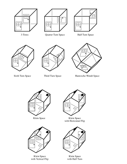
Figure 1: Fundamental domains for the compact flat three-manifolds. The unmarked walls are glued straight across. Courtesy of Adam Weeks Marano (first published in Ref. [39]).

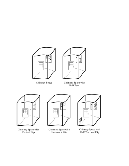
Figure 2: The chimney space is made from an infinitely tall rectangular chimney with front and back faces (resp. left and right faces) glued straight across. The four variations on the chimney space space glue the front face to the back as indicated by the doors. In all variations except the last the left and right faces are glued straight across; in the last variation they are glued with a top-to-bottom flip so that the windows match. (Courtesy of Adam Weeks Marano)

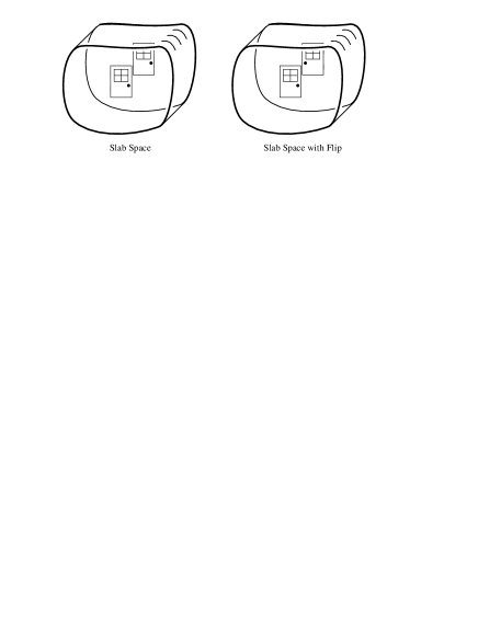
Figure 3: The slab space is made from an infinitely tall and wide slab of space with its front face glued to its back face straight across. The variation glues the faces with a flip. (Courtesy of Adam Weeks Marano)

Symbol	Name	# Compact Directions	Orientable
$E_{1}$	3-torus	3	Yes
$E_{2}$	half turn space	3	Yes
$E_{3}$	quarter turn space	3	Yes
$E_{4}$	third turn space	3	Yes
$E_{5}$	sixth turn space	3	Yes
$E_{6}$	Hantzsche-Wendt space	3	Yes
$E_{7}$	Klein space	3	No
$E_{8}$	Klein space with horizontal flip	3	No
$E_{9}$	Klein space with vertical flip	3	No
$E_{10}$	Klein space with half turn	3	No
$E_{11}$	chimney space	2	Yes
$E_{12}$	chimney space with half turn	2	Yes
$E_{13}$	chimney space with vertical flip	2	No
$E_{14}$	chimney space with horizontal flip	2	No
$E_{15}$	chimney space with half turn and flip	2	No
$E_{16}$	slab space	1	Yes
$E_{17}$	slab space with flip	1	No
$E_{18}$	Euclidean space	0	Yes

Table 1: Classification of the 18 three-dimensional flat spaces.

III Eigenmodes of ${{\bf{E}}}^{3}$

The eigenmodes of Euclidean space ${{\bf{E}}}^{3}$ admit two different bases: a basis of planar waves and a basis of spherical waves. The former are more convenient when seeking eigenbases for multi-connected spaces, while the latter are more convenient for simulating CMB maps. This section considers both bases and the conversion between them, as also detailed in the particular case of the torus in Ref. [1].

III.1 Planar waves

Each vector ${\bf k}$ defines a planar wave

$$\Upsilon_{\bf k}({\bf x})={\rm e}^{i{\bf k}\cdot{\bf x}}.$$ (4)

The defining vector ${\bf k}$, called the wave vector, lives in the dual space, so the dot product ${\bf k}\cdot{\bf x}$ is always dimensionless. These modes are indeed not square integrable and are normalized as

$$\int_{{{\bf{R}}}^{3}}\Upsilon_{\bf k}({\bf x})\Upsilon_{{\bf k}^{\prime}}^{*}({\bf x})\frac{{\rm d}^{3}{\bf x}}{(2\pi)^{3}}=\delta^{{\rm D}}({{\bf k}-{\bf k}^{\prime}}).$$ (5)

III.2 Spherical waves

Each spherical wave factors into a radial part and an angular part,

$${\cal Y}_{k\ell m}(\chi,\theta,\varphi)=\sqrt{\frac{2}{\pi}}\,(2\pi)^{3/2}\,j_{\ell}(k\chi)\,Y_{\ell}^{m}(\theta,\varphi),$$ (6)

where $(\chi,\theta,\varphi)$ are the usual spherical coordinates

$$x = \chi\;\sin{\theta}\;\cos{\varphi}$$

$$y = \chi\;\sin{\theta}\;\sin{\varphi}$$

$$z = \chi\;\cos{\theta}.$$ (7)

The radial factor $j_{\ell}(k\chi)$ is the spherical Bessel function of index $\ell$, and the angular factor $Y_{\ell}^{m}(\theta,\varphi)$ is the standard spherical harmonic. The mode ${\cal Y}_{k\ell m}$ is not square integrable and is normalized according to

$$\int_{{{\bf{R}}}^{3}}{\cal Y}_{k\ell m}{\cal Y}_{k^{\prime}\ell^{\prime}m^{\prime}}^{*}\frac{\chi^{2}{\rm d}\chi{\rm d}\cos\theta{\rm d}\varphi}{(2\pi)^{3}}=\frac{1}{k^{2}}\delta^{{\rm D}}({k-k^{\prime}})\delta_{{\ell}\,{\ell^{\prime}}}\delta_{{m}\,{m^{\prime}}},$$ (8)

which is analogous to the normalization (5) and which determines the numerical coefficient $\sqrt{2/\pi}$.

III.3 Conversion

Subsequent sections will find explicit bases for the eigenmodes of multi-connected flat three-manifolds as linear combinations of planar waves. The planar waves may easily be converted to spherical waves using Eqns 5.17.3.14 and 5.17.2.9 of Ref. [40]:

$$\Upsilon_{\bf k}({\bf x}) = {\rm e}^{i{\bf k}\cdot{\bf x}}$$ (9)

$$= \sum_{\ell=0}^{\infty}\;i^{\ell}\;j_{\ell}(k\,|{\bf x}|)\;(2\ell+1)\;P_{\ell}(\cos{\theta_{{\bf k},{\bf x}}})$$

$$= \sum_{\ell=0}^{\infty}\;i^{\ell}\;j_{\ell}(k\,|{\bf x}|)\;\left(4\pi\sum_{m=-\ell}^{\ell}Y_{\ell}^{m}({\bf\hat{x}})Y_{\ell}^{m*}({\bf\hat{k}})\right)$$

$$= \sum_{\ell=0}^{\infty}\,\sum_{m=-\ell}^{\ell}\;i^{\ell}\;Y_{\ell}^{m*}({\bf\hat{k}})\;\left[\;4\pi\;j_{\ell}(k\,|{\bf x}|)\;Y_{\ell}^{m}({\bf\hat{x}})\;\right]$$

$$= \sum_{\ell=0}^{\infty}\,\sum_{m=-\ell}^{\ell}\;\left(\;i^{\ell}\;Y_{\ell}^{m*}({\bf\hat{k}})\right){\cal Y}_{klm}({\bf x}),$$

where $k=|{\bf k}|$, ${\bf\hat{k}}\equiv{\bf k}/|{\bf k}|$, and ${\bf\hat{x}}\equiv{\bf x}/|{\bf x}|$.

In particular, the conversion formula (9) lets one easily translate a planar wave $\Upsilon_{\bf k}$ to the framework we developed in Ref. [1], which expresses each basis eigenmode as a sum of spherical waves

$$\Upsilon_{\bf k}=\Upsilon_{k,s}=\sum_{\ell=0}^{\infty}\sum_{m=-\ell}^{\ell}\xi^{s}_{k\ell m}{\cal Y}_{k\ell m},$$ (10)

where $s$ indexes the different $\Upsilon_{\bf k}$ whose wave vectors ${\bf k}$ share the same modulus $k$. In the Euclidean case the index may be chosen to be $s=\hat{\bf k}$. Comparison with (9) immediately gives the coefficients

$$\xi^{\hat{\bf k}}_{k\ell m}=i^{\ell}\;Y_{\ell}^{m*}({\bf\hat{k}}).$$ (11)

IV Eigenmodes of Multi-Connected Spaces

A multi-connected flat three-manifold is the quotient ${{\bf{E}}}^{3}/\Gamma$ of Euclidean space ${{\bf{E}}}^{3}$ under the action of a group $\Gamma$ of isometries. The group $\Gamma$ is called the holonomy group and is always discrete and fixed point free. Each eigenmode $\hat{\Upsilon}$ of the multi-connected space ${{\bf{E}}}^{3}/\Gamma$ lifts to a $\Gamma$-periodic eigenmode $\Upsilon$ of ${{\bf{E}}}^{3}$, that is, to an eigenmode of ${{\bf{E}}}^{3}$ that is invariant under the action of the holonomy group $\Gamma$. Common practice blurs the distinction between eigenmodes of ${{\bf{E}}}^{3}/\Gamma$ and $\Gamma$-periodic eigenmodes of ${{\bf{E}}}^{3}$, and we follow that practice here. Thus the task of finding the eigenmodes of the multi-connected space ${{\bf{E}}}^{3}/\Gamma$ becomes the task of finding the $\Gamma$-periodic eigenmodes of ${{\bf{E}}}^{3}$. In this section we investigate how an isometry $\gamma\in\Gamma$ acts on the space of eigenmodes. The two lemmas we obtain will make it easy to determine the eigenmodes of specific multi-connected spaces in subsequent sections.

Every isometry $\gamma$ of Euclidean space ${{\bf{E}}}^{3}$ factors as a rotation/reflection followed by a translation. If we write the rotation/reflection as a $3\times 3$ matrix $M$ in the orthogonal group ${\rm O}(3)$ and write the translation as a vector ${\bf T}$, then $\gamma$ acts on ${{\bf{E}}}^{3}$ as

$$\left(\begin{array}[]{c}{x}\\ {y}\\ {z}\end{array}\right)\quad\mapsto\quad\left(\begin{array}[]{rrr}{M_{xx}}&{M_{xy}}&{M_{xz}}\\ {M_{yx}}&{M_{yy}}&{M_{yz}}\\ {M_{zx}}&{M_{zy}}&{M_{zz}}\end{array}\right)\left(\begin{array}[]{c}{x}\\ {y}\\ {z}\end{array}\right)+\left(\begin{array}[]{c}{T_{x}}\\ {T_{y}}\\ {T_{z}}\end{array}\right).$$ (12)

This isometry of ${{\bf{E}}}^{3}$ induces a natural action $\Upsilon_{\bf k}({\bf x})\mapsto\Upsilon_{\bf k}(M{\bf x}+{\bf T})$ on the space of eigenmodes.

Lemma 1 (Action Lemma). The natural action of an isometry $\gamma$ of ${{\bf{E}}}^{3}$ takes a planar eigenmode $\Upsilon_{\bf k}$ to another planar eigenmode ${\rm e}^{i{\bf k}\cdot{\bf T}}\Upsilon_{{\bf k}M}$.

Proof. Keeping in mind that ${\bf k}$ is a row vector while ${\bf x}$ is a column vector, the proof is an easy computation:

$$\Upsilon_{\bf k}({\bf x}) = {\rm e}^{i{\bf k}\cdot{\bf x}}$$ (13)

$$\mapsto {\rm e}^{i{\bf k}\cdot(M{\bf x}+{\bf T})}$$

$$= {\rm e}^{i{\bf k}\cdot{\bf T}}\;{\rm e}^{i{\bf k}M{\bf x}}$$

$$= {\rm e}^{i{\bf k}\cdot{\bf T}}\;\Upsilon_{{\bf k}M}({\bf x}).$$

Q.E.D.

Lemma 2 (Invariance Lemma). If $\gamma$ is an isometry of ${{\bf{E}}}^{3}$ with matrix part $M$ and translational part $T$, the mode $\Upsilon_{\bf k}$ is a planar wave, and $n$ is the smallest positive integer such that ${\bf k}={\bf k}M^{n}$ (typically $n$ is simply the order of the matrix $M$), then the action of $\gamma$

1. preserves the $n$-dimensional space of eigenmodes spanned by $\{\Upsilon_{\bf k},\Upsilon_{{\bf k}M},\ldots,\Upsilon_{{\bf k}M^{n-1}}\}$ as a set, and

2. fixes a specific element

   $$a_{0}\Upsilon_{\bf k}+a_{1}\Upsilon_{{\bf k}M}+\ldots+a_{n-1}\Upsilon_{{\bf k}M^{n-1}},$$ (14)

   if and only if for each $j\mbox{ (mod }{n})$

   $$a_{j+1}={\rm e}^{i{\bf k}M^{j}{\bf T}}a_{j}.$$ (15)

Proof. Both parts are immediate corollaries of Lemma 1. Specifically, the action of $\gamma$ takes a linear combination

$$a_{0}\Upsilon_{\bf k}+a_{1}\Upsilon_{{\bf k}M}+\ldots+a_{n-2}\Upsilon_{{\bf k}M^{n-2}}+a_{n-1}\Upsilon_{{\bf k}M^{n-1}},$$ (16)

to

$$a_{0}{\rm e}^{i{\bf k}{\bf T}}\Upsilon_{{\bf k}M}+a_{1}{\rm e}^{i{\bf k}M{\bf T}}\Upsilon_{{\bf k}M^{2}}+\ldots+a_{n-2}{\rm e}^{i{\bf k}M^{n-2}{\bf T}}\Upsilon_{{\bf k}M^{n-1}}+a_{n-1}{\rm e}^{i{\bf k}M^{n-1}{\bf T}}\Upsilon_{{\bf k}},$$ (17)

so it’s clear that the $n$-dimensional subspace spanned by $\{\Upsilon_{\bf k},\Upsilon_{{\bf k}M},\ldots,\Upsilon_{{\bf k}M^{n-1}}\}$ is preserved as a set. Equating (16) to (17) and comparing coefficients proves the second part. Q.E.D.

V Compact Flat Three-Manifolds

We will first find the eigenmodes of the 3-torus, and then use them to find the eigenmodes of the remaining compact flat three-manifolds.

V.1 3-Torus

The 3-torus is the quotient of Euclidean space ${{\bf{E}}}^{3}$ under the action of three linearly independent translations ${\bf T}_{1}$, ${\bf T}_{2}$ and ${\bf T}_{3}$. Its fundamental domain is a parallelepiped. Its eigenmodes are the eigenmodes of ${{\bf{E}}}^{3}$ invariant under the translations ${\bf T}_{1}$, ${\bf T}_{2}$ and ${\bf T}_{3}$ (recall from Section IV the convention that eigenmodes of the quotient are represented as periodic eigenmodes of ${{\bf{E}}}^{3}$). The Invariance Lemma (with $n=1$) implies that an eigenmode $\Upsilon_{\bf k}$ of ${{\bf{E}}}^{3}$ is invariant under the translation ${\bf T}_{1}$ if and only if ${\rm e}^{i{\bf k}\cdot{\bf T}_{1}}=1$ which occurs precisely when ${\bf k}\cdot{\bf T}_{1}$ is an integer multiple of $2\pi$. Thus geometrically the allowed values of the wave vector ${\bf k}$ form a family of parallel planes orthogonal to ${\bf T}_{1}$. Similarly, the eigenmode $\Upsilon_{\bf k}$ is invariant under the translation ${\bf T}_{2}$ (resp. ${\bf T}_{3}$) if and only if ${\bf k}$ lies on a family of parallel planes orthogonal to ${\bf T}_{2}$ (resp. ${\bf T}_{3}$), defined by ${\bf k}\cdot{\bf T}_{2}\in 2\pi Z$ (resp. ${\bf k}\cdot{\bf T}_{3}\in 2\pi Z$). The eigenmode $\Upsilon_{\bf k}$ is invariant under all three translations ${\bf T}_{1}$, ${\bf T}_{2}$ and ${\bf T}_{3}$ if and only if it lies on all three families of parallel planes simultaneously. The intersection of the three families forms a lattice of discrete points. Fig. 4 illustrates the construction for the 2-torus; the construction for the 3-torus is analogous. This lattice of points defines the standard basis for the eigenspace of a torus.

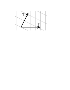
Figure 4: An eigenmode $\Upsilon_{\bf k}$ of ${{\bf{E}}}^{2}$ is invariant under the translation ${\bf T}_{i}$ if and only if ${\bf k}$ lies on a family of parallel lines orthogonal to ${\bf T}_{i}$, defined by ${\bf k}\cdot{\bf T}_{i}\in 2\pi Z$. The mode $\Upsilon_{\bf k}$ is invariant under both translations ${\bf T}_{1}$ and ${\bf T}_{2}$ if and only if it lies in the lattice of intersection points of the two families of parallel lines. The construction in three dimensions is similar, but with three families of planes instead of two families of lines. Strictly speaking we should not draw the parallel lines in the same space as the translation vectors ${\bf T}_{i}$ because the wave vectors ${\bf k}$ live in the dual space (with units of $\,{\mbox{length}^{-1}}$) while the ${\bf T}_{i}$ live in the primary space (with units of  length), but nevertheless it’s visually helpful to do so.

Definition. The standard basis for a 3-torus ${{\bf{T}}}^{3}$ generated by three linearly independent translations ${\bf T}_{1}$, ${\bf T}_{2}$ and ${\bf T}_{3}$ is the set $B=\{\Upsilon_{\bf k}\;|\;{\bf k}\cdot{\bf T}_{i}\in 2\pi Z\mbox{ for }i=1,2,3\}$.

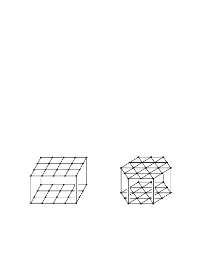
Figure 5: In a rectangular 3-torus (left) the allowed wave vectors ${\bf k}$ form a rectangular lattice. In a hexagonal 3-torus (right) the lattice is hexagonal within each layer.

The most important special case of a 3-torus is the rectangular 3-torus generated by three mutually orthogonal translations

$${\bf T}_{1} = (L_{x},0,0)$$

$${\bf T}_{2} = (0,L_{y},0)$$

$${\bf T}_{3} = (0,0,L_{z}),$$ (18)

in which case the allowed wave vectors ${\bf k}$ take the form

$${\bf k}=2\pi\,\left(\frac{n_{x}}{L_{x}},\,\frac{n_{y}}{L_{y}},\,\frac{n_{z}}{L_{z}}\right),$$ (19)

for integer values of $n_{x}$, $n_{y}$ and $n_{z}$, thus forming a rectangular lattice (Fig. 5 left).

The second most important special case is the hexagonal 3-torus generated by

$${\bf T}_{1} = \left(L,0,0\right)$$

$${\bf T}_{2} = \left(-\frac{1}{2}L,+\frac{\sqrt{3}}{2}L,0\right)$$

$${\bf T}_{3} = \left(-\frac{1}{2}L,-\frac{\sqrt{3}}{2}L,0\right)$$

$${\bf T}_{4} = \left(0,0,L_{z}\right).$$ (20)

These four generators and their inverses define a fundamental domain as a hexagonal prism. The first three generators are linearly dependent (${\bf T}_{1}+{\bf T}_{2}+{\bf T}_{3}=0$); eliminating any one of them suggests an alternative fundamental domain as a prism with a rhombic base. Even though the hexagonal and rhombic prisms look different, they define the same manifold. Either way, the allowed wave vectors ${\bf k}$ form a hexagonal lattice (Fig. 5 right) and may be parameterized as

$${\bf k}\quad=\quad 2\pi\,\left(-\frac{n_{1}}{L},\frac{2n_{1}-n_{2}}{\sqrt{3}L},\frac{n_{3}}{L_{z}}\right),$$ (21)

for integer values of $n_{1}$, $n_{2}$ and $n_{3}$.

In the case of a general 3-torus, one writes the translations ${\bf T}_{1}$, ${\bf T}_{2}$ and ${\bf T}_{3}$ as the columns of a $3\times 3$ matrix $T$ and solves the equation ${\bf k}T=2\pi(n_{1},n_{2},n_{3})$ to find the allowable wave vectors ${\bf k}=2\pi(n_{1},n_{2},n_{3})T^{-1}$ for integers $n_{1}$, $n_{2}$ and $n_{3}$.

When one wants to simulate CMB maps, one needs to know not only the modes themselves but also how the modes are paired under complex conjugation. The reason is that the cosmological fields are in fact real-valued stochastic variables. Any such field can be decomposed into Fourier modes as

$$\phi({\bf x},t)=\int\frac{{\rm d}^{3}{\bf k}}{(2\pi)^{3/2}}\phi_{\bf k}(t){\rm e}^{i{\bf k}.{\bf x}}\hat{e}_{\bf k},$$ (22)

where $\hat{e}_{\bf k}$ is a complex, usually Gaussian, random variable satisfying

$$\left<\hat{e}_{\bf k}\hat{e}_{{\bf k}^{\prime}}^{*}\right>=\delta^{{\rm D}}({{\bf k}-{\bf k}^{\prime}}).$$ (23)

The evolution equations of the cosmological perturbations involve time derivatives and a Laplacian so that the coefficient $\phi_{\bf k}(t)$ can be decomposed as

$$\phi_{\bf k}(t)=\phi_{k}(t){\rm e}^{i\theta_{\bf k}},$$ (24)

where $\theta_{\bf k}$ is a phase that is constant throughout the evolution. By absorbing the phase into the random variable, we can always choose $\phi_{\bf k}$ to be a real function of $k$ only, i.e., $\phi_{k}(t)$. Since ${\rm e}^{i{\bf k}\cdot{\bf x}}$ and ${\rm e}^{-i{\bf k}\cdot{\bf x}}$ are conjugate in the preceding decomposition, the fact that $\phi({\bf x},t)$ is real implies that

$$\hat{e}_{\bf k}^{*}=\hat{e}_{-{\bf k}}.$$ (25)

This latter constraint may not hold for all the other spaces studied in this article and we will need to give its analog for each case.

V.2 Quotients of the 3-Torus

For ease of illustration we first explain our general method for the two-dimensional Klein bottle. Figure 6 shows a portion of the Klein bottle’s universal cover, in which alternate images of the fundamental domain appear mirror reversed. Half the holonomies are pure translations while the other half are glide reflections. In other words, the holonomy group $\Gamma$ contains an index 2 subgroup $\Gamma^{\prime}\subset\Gamma$ comprising the pure translations. While ${{\bf{E}}}^{2}/\Gamma$ gives the original Klein bottle, ${{\bf{E}}}^{2}/\Gamma^{\prime}$ gives a torus whose fundamental domain is the square formed by the solid lines in Figure 6 (ignoring the dotted lines). According to the convention introduced in Section IV, the Klein bottle’s eigenmodes are represented as $\Gamma$-periodic functions on ${{\bf{E}}}^{2}$. But every $\Gamma$-periodic function is automatically a $\Gamma^{\prime}$-periodic function as well, because $\Gamma^{\prime}$ is a subgroup of $\Gamma$. Thus every eigenmode of the Klein bottle is a priori an eigenmode of the 2-torus. The task in finding the eigenspace of the Klein bottle is to start with the eigenspace of the torus and find the subspace that is invariant under the glide reflection (the one taking the lower half of a square to the upper half). In practice this is quite simple. A rectangular torus has holonomy group $\Gamma^{\prime}$ generated by the two translations

$$\left(\begin{array}[]{c}{x}\\ {y}\end{array}\right)\;\mapsto\;\left(\begin{array}[]{c}{x}\\ {y}\end{array}\right)+\left(\begin{array}[]{c}{L_{x}}\\ {0}\end{array}\right)\qquad\mbox{and}\qquad\left(\begin{array}[]{c}{x}\\ {y}\end{array}\right)\;\mapsto\;\left(\begin{array}[]{c}{x}\\ {y}\end{array}\right)+\left(\begin{array}[]{c}{0}\\ {L_{y}}\end{array}\right).$$ (26)

The standard eigenbasis for this torus takes the form (19), namely $B=\{\Upsilon_{\bf k}\;|\;{\bf k}=2\pi(\frac{n_{x}}{L_{x}},\frac{n_{y}}{L_{y}})\mbox{ for }n_{x},n_{y}\in Z\}$. To extend this $\Gamma^{\prime}$ to the full holonomy group $\Gamma$ of the Klein bottle, we add the glide reflection

$$\left(\begin{array}[]{c}{x}\\ {y}\end{array}\right)\;\mapsto\;\left(\begin{array}[]{rrr}{-1}&{0}\\ {0}&{1}\end{array}\right)\left(\begin{array}[]{c}{x}\\ {y}\end{array}\right)+\left(\begin{array}[]{c}{0}\\ {L_{y}/2}\end{array}\right),$$ (27)

and ask which elements of the basis $B$ it preserves. The Invariance Lemma provides a ready answer: when $k_{x}\neq 0$ the two-dimensional subspace $\{\Upsilon_{k_{x},k_{y}},\Upsilon_{-k_{x},k_{y}}\}$ is preserved as a set (Part 1 of the Invariance Lemma) while the mode $\Upsilon_{k_{x},k_{y}}+(-1)^{n_{y}}\Upsilon_{-k_{x},k_{y}}$ is fixed exactly (Part 2 of the Invariance Lemma). In the exceptional case that $k_{x}=0$, the one-dimensional subspace $\{\Upsilon_{0,k_{y}}\}$ is preserved as a set, while $\Upsilon_{0,k_{y}}$ is fixed if and only if $n_{y}$ is even (because when $n=1$, Part 2 of the Invariance Lemma requires $a_{0}={\rm e}^{i{\bf k}\cdot{\bf T}}a_{0}$ which implies ${\bf k}\cdot{\bf T}/(2\pi)=n_{z}/2\in Z$). In summary, an orthonormal basis for the space of eigenmodes of the Klein bottle is the union of

$$\begin{array}[]{lcl}\left[\Upsilon_{2\pi(\frac{n_{x}}{L_{x}},\frac{n_{y}}{L_{y}})}+(-1)^{n_{y}}\Upsilon_{2\pi(-\frac{n_{x}}{L_{x}},\frac{n_{y}}{L_{y}})}\right]/\sqrt{2}&\quad\mbox{for}&n_{x}\in Z^{+},n_{y}\in Z,\\ \Upsilon_{2\pi(0,\frac{n_{y}}{L_{y}})}&\quad\mbox{for}&n_{y}\in 2Z.\\ \end{array}$$ (28)

Figure 6: The Klein bottle’s holonomy group contains glide reflections as well as translations. The translations alone form an index 2 subgroup defining a torus.

Let us now apply this same method to each of the nine quotients of the 3-torus.

V.2.1 Half turn space

The analysis of the half turn space closely follows that of the Klein bottle given immediately above. The only difference is that the Klein bottle’s holonomy group contained translations and glide reflections, while the half turn space’s holonomy group contains translations and corkscrew motions. Specifically, we begin with the generators for the holonomy group $\Gamma^{\prime}$ of a rectangular 3-torus

$$\left(\begin{array}[]{c}{x}\\ {y}\\ {z}\end{array}\right)\;\mapsto\;\left(\begin{array}[]{c}{x}\\ {y}\\ {z}\end{array}\right)+\left(\begin{array}[]{c}{L_{x}}\\ {0}\\ {0}\end{array}\right),\qquad\left(\begin{array}[]{c}{x}\\ {y}\\ {z}\end{array}\right)\;\mapsto\;\left(\begin{array}[]{c}{x}\\ {y}\\ {z}\end{array}\right)+\left(\begin{array}[]{c}{0}\\ {L_{y}}\\ {0}\end{array}\right),\qquad\left(\begin{array}[]{c}{x}\\ {y}\\ {z}\end{array}\right)\;\mapsto\;\left(\begin{array}[]{c}{x}\\ {y}\\ {z}\end{array}\right)+\left(\begin{array}[]{c}{0}\\ {0}\\ {L_{z}}\end{array}\right).$$ (29)

and add a generator for the half-turn corkscrew motion

$$\left(\begin{array}[]{c}{x}\\ {y}\\ {z}\end{array}\right)\;\mapsto\;\left(\begin{array}[]{rrr}{-1}&{0}&{0}\\ {0}&{-1}&{0}\\ {0}&{0}&{\;\;\;1}\end{array}\right)\left(\begin{array}[]{c}{x}\\ {y}\\ {z}\end{array}\right)+\left(\begin{array}[]{c}{0}\\ {0}\\ {L_{z}/2}\end{array}\right),$$ (30)

to get the full holonomy group $\Gamma$ of the half turn space. The Invariance Lemma shows that when $(k_{x},k_{y})\neq(0,0)$ the two-dimensional subspace $\{\Upsilon_{k_{x},k_{y},k_{z}},\Upsilon_{-k_{x},-k_{y},k_{z}}\}$ is preserved as a set (Part 1 of the Invariance Lemma) while the mode $\Upsilon_{k_{x},k_{y},k_{z}}+(-1)^{n_{z}}\Upsilon_{-k_{x},-k_{y},k_{z}}$ is fixed exactly (Part 2 of the Invariance Lemma). In the exceptional case that $(k_{x},k_{y})=(0,0)$, the one-dimensional subspace $\{\Upsilon_{0,0,k_{z}}\}$ is preserved as a set, while $\Upsilon_{0,0,k_{z}}$ is fixed if and only if $n_{z}$ is even. In summary, an orthonormal basis for the space of eigenmodes of the half turn space, $\Upsilon_{k_{x},k_{y},k_{z}}^{[E_{2}]}$, is the union of

$$\begin{array}[]{lcl}\frac{1}{\sqrt{2}}\left[\Upsilon_{2\pi(\frac{n_{x}}{L_{x}},\frac{n_{y}}{L_{y}},\frac{n_{z}}{L_{z}})}+(-1)^{n_{z}}\Upsilon_{2\pi(-\frac{n_{x}}{L_{x}},-\frac{n_{y}}{L_{y}},\frac{n_{z}}{L_{z}})}\right]&\quad\mbox{for}&(n_{x}\in Z^{+},n_{y},n_{z}\in Z)\mbox{ or }(n_{x}=0,n_{y}\in Z^{+},n_{z}\in Z),\\ \Upsilon_{2\pi(0,0,\frac{n_{z}}{L_{z}})}&\quad\mbox{for}&n_{z}\in 2Z.\\ \end{array}$$ (31)

In terms of the notations used in Ref. [1], it leads to the coefficients

$$\xi_{k\ell m}^{\hat{\bf k}}=\left\{\begin{array}[]{lcl}\frac{i^{\ell}}{\sqrt{2}}\left[Y_{\ell}^{m*}(\hat{\bf k})+(-1)^{n_{z}}Y_{\ell}^{m*}(\hat{\bf k}M)\right]&\quad\mbox{for}&(n_{x}\in Z^{+},n_{y},n_{z}\in Z)\mbox{ or }(n_{x}=0,n_{y}\in Z^{+},n_{z}\in Z),\\ i^{\ell}Y_{\ell}^{m*}(\hat{\bf k})&\quad\mbox{for}&(n_{x},n_{y})=(0,0),\quad n_{z}\in 2Z.\\ \end{array}\right.,$$ (32)

${\bf k}$ being given by Eq. (19). Passing from the expression of the modes to the coefficients $\xi^{{\hat{\bf k}}}_{{k}\,{\ell}\,{m}}$ is straightforward and in the following we will give only the expressions of the modes.

If desired, one could construct a more general half turn space from a right prism with a parallelogram base, instead of a rectangular box.

To find the analog of Eq. (25), one simply needs to check that

$$\Upsilon_{k_{x},k_{y},k_{z}}^{[E_{2}]*}=(-1)^{n_{z}}\Upsilon_{k_{x},k_{y},-k_{z}}^{[E_{2}]},$$ (33)

so that it follows that

1. when $k_{z}\not=0$, $\hat{e}_{\bf k}$ is a complex random variable satisfying

   $$\hat{e}_{k_{x},k_{y},k_{z}}^{*}=(-1)^{n_{z}}\hat{e}_{k_{x},k_{y},-k_{z}},$$ (34)

2. when $k_{z}=0$, $\hat{e}_{\bf k}$ is a real random variable.

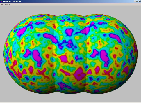
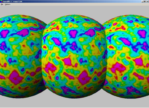
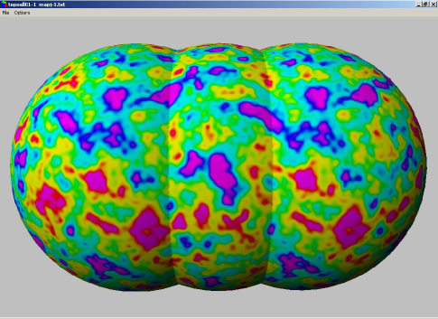
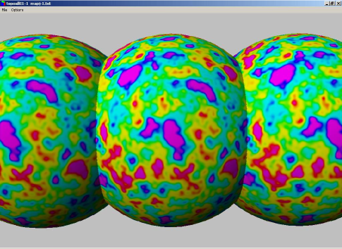
Figure 7: The last scattering surface seen from outside for a half-turn space $E_{2}$ with $L_{x}=L_{y}=0.64$, $L_{z}=1.28$ in units of the radius of the last scattering surface. Each row presents the two pairs of matching circles along the $z$ direction, but seen from opposite directions. The left panels show circles which match with a $\pi$ rotation while the right panel shows circles which match without rotation. We recover the invariance by a translation of $L_{z}$ due to the fact that the cubic torus of size $L_{z}=1.28$ is the double cover of the half-turn space considered here. Only the Sachs-Wolfe contribution has been depicted here.

V.2.2 Quarter turn space

The quarter turn space is similar to the half turn space, but with with a quarter turn corkscrew motion

$$\left(\begin{array}[]{c}{x}\\ {y}\\ {z}\end{array}\right)\;\mapsto\;\left(\begin{array}[]{rrr}{0}&{-1}&{0}\\ {1}&{0}&{0}\\ {0}&{0}&{1}\end{array}\right)\left(\begin{array}[]{c}{x}\\ {y}\\ {z}\end{array}\right)+\left(\begin{array}[]{c}{0}\\ {0}\\ {L_{x}/4}\end{array}\right).$$ (35)

In particular this implies that $L_{x}=L_{y}$. The Invariance Lemma shows that when $(k_{x},k_{y})\neq(0,0)$ the four-dimensional subspace $\{\Upsilon_{k_{x},k_{y},k_{z}}$, $\Upsilon_{k_{y},-k_{x},k_{z}}$, $\Upsilon_{-k_{x},-k_{y},k_{z}}$, $\Upsilon_{-k_{y},k_{x},k_{z}}\}$ is preserved as a set, while the mode $\Upsilon_{k_{x},k_{y},k_{z}}+i^{n_{z}}\Upsilon_{k_{y},-k_{x},k_{z}}+(-1)^{n_{z}}\Upsilon_{-k_{x},-k_{y},k_{z}}+(-i)^{n_{z}}\Upsilon_{-k_{y},k_{x},k_{z}}$ is fixed exactly. In the exceptional case that $(k_{x},k_{y})=(0,0)$, the one-dimensional subspace $\{\Upsilon_{0,0,k_{z}}\}$ is preserved as a set, while $\Upsilon_{0,0,k_{z}}$ is fixed if and only if $n_{z}$ is a multiple of 4. In summary, an orthonormal basis for the space of eigenmodes of the quarter turn space, $\Upsilon_{k_{x},k_{y},-k_{z}}^{[E_{3}]}$, is the union of

$$\frac{1}{2}\left[\Upsilon_{2\pi(\frac{n_{x}}{L_{x}},\frac{n_{y}}{L_{y}},\frac{n_{z}}{L_{z}})}+i^{n_{z}}\Upsilon_{2\pi(\frac{n_{y}}{L_{y}},-\frac{n_{x}}{L_{x}},\frac{n_{z}}{L_{z}})}+i^{2n_{z}}\Upsilon_{2\pi(-\frac{n_{x}}{L_{x}},-\frac{n_{y}}{L_{y}},\frac{n_{z}}{L_{z}})}+i^{3n_{z}}\Upsilon_{2\pi(-\frac{n_{y}}{L_{y}},\frac{n_{x}}{L_{x}},\frac{n_{z}}{L_{z}})}\right]$$

$$\qquad\qquad\mbox{for}\quad n_{x}\in Z^{+},n_{y}\in Z^{+}\cup\{0\},n_{z}\in Z,$$

$$\Upsilon_{2\pi(0,0,\frac{n_{z}}{L_{z}})}\quad\mbox{for}\quad n_{z}\in 4Z.$$ (36)

As in the case of the half turn space, one can easily check that

$$\Upsilon_{k_{x},k_{y},k_{z}}^{[E_{3}]*}=(-1)^{n_{z}}\Upsilon_{k_{x},k_{y},-k_{z}}^{[E_{3}]},$$ (37)

so that the analog of Eq. (25) is given by

1. when $k_{z}\not=0$, $\hat{e}_{\bf k}$ is a complex random variable satisfying

   $$\hat{e}_{k_{x},k_{y},k_{z}}^{*}=(-1)^{n_{z}}\hat{e}_{k_{x},k_{y},-k_{z}},$$ (38)

2. when $k_{z}=0$, $\hat{e}_{\bf k}$ is a real random variable.

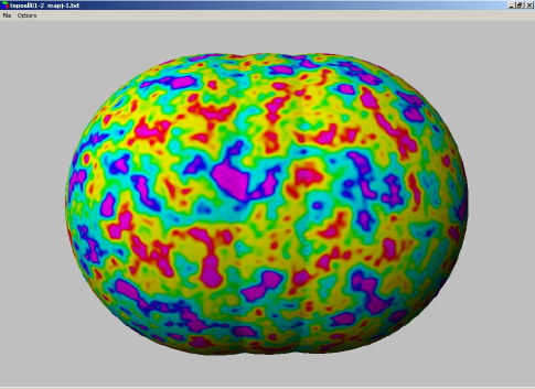
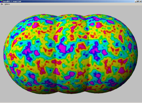
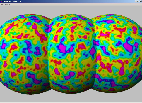
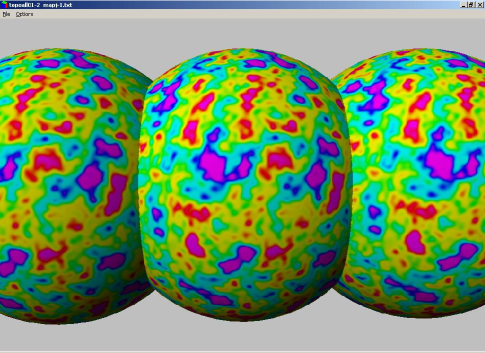
Figure 8: The last scattering surface seen from outside for a quarter-turn space $E_{3}$ with $L_{x}=L_{y}=0.64$ and $L_{z}=1.28$. We present the four pairs of matched circles along the $z$-axis, which match with a twist of $\pi/2$, $\pi$, $3\pi/2$ and $2\pi$, respectively. We recover the invariance by a translation of $L_{z}$ for the last pair due to the fact that the cubic torus of size $L_{z}=1.28$ is the four-fold cover of the quarter-turn space considered here. Only the Sachs-Wolfe contribution has been depicted here.

V.2.3 Third turn space

The third turn space is a three-fold quotient of a hexagonal 3-torus, not a rectangular one. To the generators (V.1) of the hexagonal 3-torus we add a one-third turn corkscrew motion

$$\left(\begin{array}[]{c}{x}\\ {y}\\ {z}\end{array}\right)\;\mapsto\;\left(\begin{array}[]{rrr}{-\frac{1}{2}}&{-\frac{\sqrt{3}}{2}}&{0}\\ {\frac{\sqrt{3}}{2}}&{-\frac{1}{2}}&{0}\\ {0}&{0}&{1}\end{array}\right)\left(\begin{array}[]{c}{x}\\ {y}\\ {z}\end{array}\right)+\left(\begin{array}[]{c}{0}\\ {0}\\ {L_{z}/3}\end{array}\right).$$ (39)

The eigenmodes $\Upsilon_{\bf k}$ of the hexagonal 3-torus are already known from Eqn. (21) (and illustrated in Figure 5). Applying the Invariance Lemma to them with the additional generator (39) yields the eigenbasis, $\Upsilon_{k_{x},k_{y},k_{z}}^{[E_{4}]}$,

$$\begin{array}[]{lcl}\frac{1}{\sqrt{3}}\left[\Upsilon_{{\bf k}}+\zeta^{n_{3}}\Upsilon_{{\bf k}M}+\zeta^{2n_{3}}\Upsilon_{{\bf k}M^{2}}\right]&\quad\mbox{for}&n_{1}\in Z^{+},\;n_{2}\in Z^{+}\cup\{0\},n_{3}\in Z,\\ \Upsilon_{2\pi(0,0,\frac{n_{3}}{L_{z}})}&\quad\mbox{for}&n_{3}\in 3Z,\\ \end{array}$$ (40)

where $\zeta={\rm e}^{2i\pi/3}$ is a cube root of unity and it is easily checked that

$${\bf k} = 2\pi\left(\frac{-n_{2}}{L},\;\frac{2n_{1}-n_{2}}{\sqrt{3}L},\;\frac{n_{3}}{L_{z}}\right)$$

$${\bf k}M = 2\pi\left(\frac{n_{1}}{L},\;\frac{2n_{2}-n_{1}}{\sqrt{3}L},\;\frac{n_{3}}{L_{z}}\right)$$

$${\bf k}M^{2} = 2\pi\left(\frac{n_{2}-n_{1}}{L},\;\frac{-n_{1}-n_{2}}{\sqrt{3}L},\;\frac{n_{3}}{L_{z}}\right).$$ (41)

One can check that

$$\Upsilon_{n_{1},n_{2},n_{3}}^{*}=\left\{\begin{array}[]{ll}\zeta^{2n_{3}}\Upsilon_{n_{2},n_{2}-n_{1},-n_{3}}&\hbox{when}\,n_{2}>n_{1}\\ \zeta^{n_{3}}\Upsilon_{n_{1}-n_{2},n_{1},-n_{3}}&\hbox{when}\,n_{1}\geq n_{2}\end{array}\right..$$ (42)

It follows that the analog of Eq. (25) is given by

1. $$\hat{e}_{n_{1},n_{2},n_{3}}^{*}=\left\{\begin{array}[]{ll}\zeta^{2n_{3}}\hat{e}_{n_{2},n_{2}-n_{1},-n_{3}}&\hbox{when}\,n_{2}>n_{1}\\ \zeta^{n_{3}}\hat{e}_{n_{1}-n_{2},n_{1},-n_{3}}&\hbox{when}\,n_{1}\geq n_{2}\end{array}\right..$$ (43)

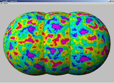
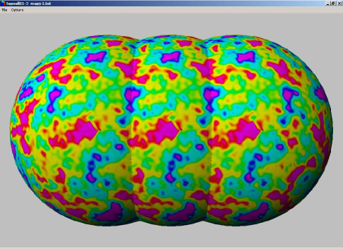
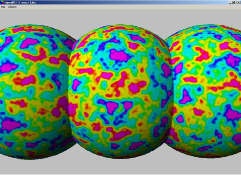
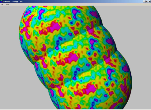
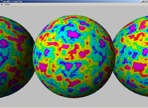
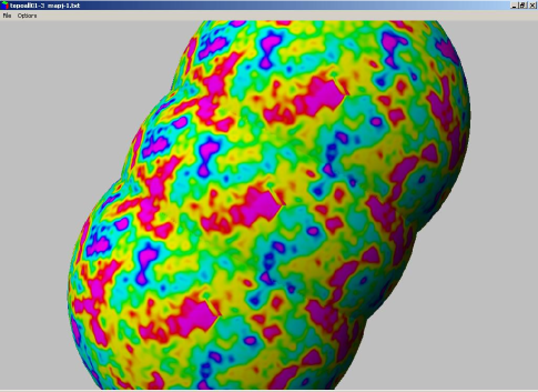
Figure 9: The last scattering surface seen from outside for a third-turn space $E_{4}$ with $L_{x}=L_{y}=0.64$ and $L_{z}=1.92$ in units of the last scattering surface. The first column presents the three pairs of circles alonq the $z$ axis which match after a rotation of $2\pi/3$, $4\pi/3$ and $2\pi$ respectively. We recover the invariance by a translation of $L_{z}$ due to the fact that the cubic torus of size $L_{z}=1.92$ is the three-fold cover of the third-turn space considered here. The second column present the three pairs of circles related by translations in the $xy$-plane. Only the Sachs-Wolfe contribution has been depicted here.

V.2.4 Sixth turn space

The sixth turn space is like the third turn space, but with a one-sixth turn corkscrew motion

$$\left(\begin{array}[]{c}{x}\\ {y}\\ {z}\end{array}\right)\;\mapsto\;\left(\begin{array}[]{rrr}{\frac{1}{2}}&{-\frac{\sqrt{3}}{2}}&{0}\\ {\frac{\sqrt{3}}{2}}&{\frac{1}{2}}&{0}\\ {0}&{0}&{1}\end{array}\right)\left(\begin{array}[]{c}{x}\\ {y}\\ {z}\end{array}\right)+\left(\begin{array}[]{c}{0}\\ {0}\\ {L_{z}/6}\end{array}\right).$$ (44)

The same reasoning as before shows the eigenbasis, $\Upsilon_{k_{x},k_{y},k_{z}}^{[E_{5}]}$, to be

$$\begin{array}[]{lcl}\frac{1}{\sqrt{6}}\left[\Upsilon_{{\bf k}}+\zeta^{n_{3}}\Upsilon_{{\bf k}M}+\zeta^{2n_{3}}\Upsilon_{{\bf k}M^{2}}+\zeta^{3n_{3}}\Upsilon_{{\bf k}M^{3}}+\zeta^{4n_{3}}\Upsilon_{{\bf k}M^{4}}+\zeta^{5n_{3}}\Upsilon_{{\bf k}M^{5}}\right]&\mbox{ for }&n_{1}\in Z^{+},\;n_{2}\in Z^{+}\cup\{0\},\;n_{2}<n_{1},n_{3}\in Z,\\ \Upsilon_{2\pi(0,0,\frac{n_{3}}{L_{z}})}&\mbox{ for }&n_{3}\in 6Z,\\ \end{array}$$ (45)

where $\zeta={\rm e}^{2i\pi/6}$ is a sixth root of unity and it is easily checked that

$${\bf k} = 2\pi\left(\frac{-n_{2}}{L},\;\frac{2n_{1}-n_{2}}{\sqrt{3}L},\;\frac{n_{3}}{L_{z}}\right)$$

$${\bf k}M = 2\pi\left(\frac{n_{1}-n_{2}}{L},\;\frac{n_{1}+n_{2}}{\sqrt{3}L},\;\frac{n_{3}}{L_{z}}\right)$$

$${\bf k}M^{2} = 2\pi\left(\frac{n_{1}}{L},\;\frac{2n_{2}-n_{1}}{\sqrt{3}L},\;\frac{n_{3}}{L_{z}}\right)$$

$${\bf k}M^{3} = 2\pi\left(\frac{n_{2}}{L},\;\frac{n_{2}-2n_{1}}{\sqrt{3}L},\;\frac{n_{3}}{L_{z}}\right)$$

$${\bf k}M^{4} = 2\pi\left(\frac{n_{2}-n_{1}}{L},\;\frac{-n_{1}-n_{2}}{\sqrt{3}L},\;\frac{n_{3}}{L_{z}}\right)$$

$${\bf k}M^{5} = 2\pi\left(\frac{-n_{1}}{L},\;\frac{n_{1}-2n_{2}}{\sqrt{3}L},\;\frac{n_{3}}{L_{z}}\right).$$ (46)

One can check that

$$\Upsilon_{n_{1},n_{2},n_{3}}^{*}=(-1)^{n_{3}}\Upsilon_{n_{1},n_{2},-n_{3}},$$ (47)

so that when $n_{3}\neq 0$ an analog relation exists with the corresponding complex random variables, and when $n_{3}=0$, the random variable $\hat{e}_{n_{1},n_{2},0}$ is real.

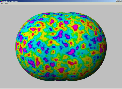
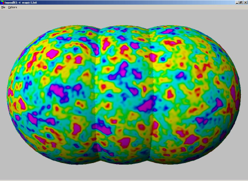
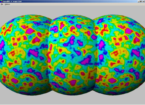
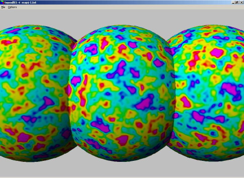
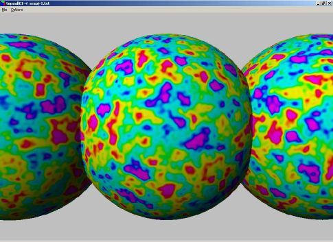
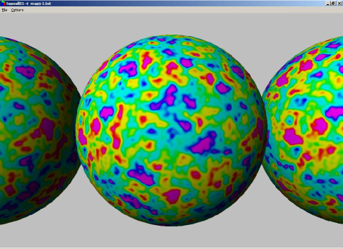
Figure 10: The last scattering surface seen from outside for a sixth-turn space $E_{5}$ with $L_{x}=L_{y}=0.64$ and $L_{z}=1.92$ in units of the last scattering surface. We presents the six pairs of circles along the $z$ axis which match after a rotation of $\pi/3$, $2\pi/3\ldots 2\pi$ respectively. We recover the invariance by a translation of $L_{z}$ due to the fact that the cubic torus of size $L_{z}=1.92$ is the six-fold cover of the sixth-turn space considered here. Only the Sachs-Wolfe contribution has been depicted here.

V.2.5 Hantzsche-Wendt space

The fundamental polyhedron of the Hantzsche-Wendt space is a rhombic dodecahedron circumscribed about a rectangular box of size $(L_{x}/2,L_{y}/2,L_{z}/2)$. The holonomy group is generated by the three half-turn corkscrew motions

$$\left(\begin{array}[]{c}{x}\\ {y}\\ {z}\end{array}\right)\; \mapsto \;\left(\begin{array}[]{rrr}{\;\;\;1}&{0}&{0}\\ {0}&{-1}&{0}\\ {0}&{0}&{-1}\end{array}\right)\left(\begin{array}[]{c}{x}\\ {y}\\ {z}\end{array}\right)+\left(\begin{array}[]{c}{L_{x}/2}\\ {L_{y}/2}\\ {0}\end{array}\right)$$ (60)

$$\left(\begin{array}[]{c}{x}\\ {y}\\ {z}\end{array}\right)\; \mapsto \;\left(\begin{array}[]{rrr}{-1}&{0}&{0}\\ {0}&{\;\;\;1}&{0}\\ {0}&{0}&{-1}\end{array}\right)\left(\begin{array}[]{c}{x}\\ {y}\\ {z}\end{array}\right)+\left(\begin{array}[]{c}{0}\\ {L_{y}/2}\\ {L_{z}/2}\end{array}\right)$$ (73)

$$\left(\begin{array}[]{c}{x}\\ {y}\\ {z}\end{array}\right)\; \mapsto \;\left(\begin{array}[]{rrr}{-1}&{0}&{0}\\ {0}&{-1}&{0}\\ {0}&{0}&{\;\;\;1}\end{array}\right)\left(\begin{array}[]{c}{x}\\ {y}\\ {z}\end{array}\right)+\left(\begin{array}[]{c}{L_{x}/2}\\ {0}\\ {L_{z}/2}\end{array}\right).$$ (86)

The composition of these three generators is the identity, so any two suffice to generate the group. Each element of the Hantzsche-Wendt group has a rotational component $M\in\{{\rm diag}(1,1,1)$, ${\rm diag}(1,-1,-1)$, ${\rm diag}(-1,1,-1)$, ${\rm diag}(-1,-1,1)\}$. The pure translations (elements with $M={\rm diag}(1,1,1)$) form a subgroup of index 4; the corresponding four-fold cover of the Hantzsche-Wendt space is a rectangular 3-torus of size $(L_{x},L_{y},L_{z})$, whose holonomy is generated by the squares of the above corkscrew motions. Thus we may begin with the eigenspace for a rectangular 3-torus (19) and ask what subspace remains fixed by the three Hantzsche-Wendt generators (86). The Invariance Lemma shows that all three generators preserve the (typically four-dimensional) subspace $\{\Upsilon_{k_{x},k_{y},k_{z}},\Upsilon_{k_{x},-k_{y},-k_{z}},\Upsilon_{-k_{x},k_{y},-k_{z}},\Upsilon_{-k_{x},-k_{y},k_{z}}\}$ as a set, and fix the linear combination

$$\Upsilon_{k_{x},k_{y},k_{z}}\;+\;(-1)^{n_{x}-n_{y}}\Upsilon_{k_{x},-k_{y},-k_{z}}\;+\;(-1)^{n_{y}-n_{z}}\Upsilon_{-k_{x},k_{y},-k_{z}}\;+\;(-1)^{n_{z}-n_{x}}\Upsilon_{-k_{x},-k_{y},k_{z}}.$$ (87)

Visualizing the four wave vectors in the subscripts of (87) as alternate corners of the cube $(\pm k_{x},\,\pm k_{y},\,\pm k_{z})=2\pi(\frac{\pm n_{x}}{L_{x}},\,\frac{\pm n_{y}}{L_{y}},\,\frac{\pm n_{z}}{L_{z}})$, one sees that subspace will be degenerate if and only if at least two of the indices $\{n_{x},n_{y},n_{z}\}$ are zero. In the degenerate case a two-dimensional subspace like $\{\Upsilon_{k_{x},0,0},\Upsilon_{-k_{x},0,0}\}$ is preserved as a set, while the mode $\Upsilon_{k_{x},0,0}+\Upsilon_{-k_{x},0,0}$ is preserved by all three generators if and only if $n_{x}$ is even. Thus the Hantzsche-Wendt’s eigenspace has basis, $\Upsilon_{k_{x},k_{y},k_{z}}^{[E_{6}]}$,

$$\frac{1}{2}\left[\Upsilon_{2\pi(\frac{n_{x}}{L_{x}},\frac{n_{y}}{L_{y}},\frac{n_{z}}{L_{z}})}+(-1)^{n_{x}-n_{y}}\Upsilon_{2\pi(\frac{n_{x}}{L_{x}},-\frac{n_{y}}{L_{y}},-\frac{n_{z}}{L_{z}})}+(-1)^{n_{y}-n_{z}}\Upsilon_{2\pi(-\frac{n_{x}}{L_{x}},\frac{n_{y}}{L_{y}},-\frac{n_{z}}{L_{z}})}+(-1)^{n_{z}-n_{x}}\Upsilon_{2\pi(-\frac{n_{x}}{L_{x}},-\frac{n_{y}}{L_{y}},\frac{n_{z}}{L_{z}})}\right]$$

$$\qquad\qquad\mbox{for}\quad(n_{x},n_{y}\in Z^{+},n_{z}\in Z)\mbox{ or }(n_{x}=0,n_{y},n_{z}\in Z^{+})\mbox{ or }(n_{y}=0,n_{x},n_{z}\in Z^{+}),$$

$$\frac{1}{\sqrt{2}}\left[\Upsilon_{2\pi(\frac{n_{x}}{L_{x}},0,0)}+\Upsilon_{2\pi(-\frac{n_{x}}{L_{x}},0,0)}\right]\quad\mbox{for}\quad n_{x}\in 2Z^{+},$$

$$\frac{1}{\sqrt{2}}\left[\Upsilon_{2\pi(0,\frac{n_{y}}{L_{y}},0)}+\Upsilon_{2\pi(0,-\frac{n_{y}}{L_{y}},0)}\right]\quad\mbox{for}\quad n_{y}\in 2Z^{+},$$

$$\frac{1}{\sqrt{2}}\left[\Upsilon_{2\pi(0,0,\frac{n_{z}}{L_{z}})}+\Upsilon_{2\pi(0,0,-\frac{n_{z}}{L_{z}})}\right]\quad\mbox{for}\quad n_{z}\in 2Z^{+}.$$ (88)

One can easily check that

$$\Upsilon_{k_{x},k_{y},k_{z}}^{[E_{6}]*}=(-1)^{n_{x}-n_{z}}\Upsilon_{k_{x},k_{y},-k_{z}}^{[E_{6}]},$$ (89)

when $(n_{x},n_{y}\in Z^{+},n_{z}\in Z)$ or $(n_{x}=0,n_{y},n_{z}\in Z^{+})$ or $(n_{y}=0,n_{x},n_{z}\in Z^{+})$ and that otherwise $\Upsilon_{k_{x},k_{y},k_{z}}^{[E_{6}]}$ is real. It follows that the analog of Eq. (25) is given by

1. when $n_{x},n_{y}\in Z^{+}$ and $n_{z}\in Z$, $\hat{e}_{\bf k}$ is a complex random variable satisfying

   $$\hat{e}_{k_{x},k_{y},k_{z}}^{*}=(-1)^{n_{x}-n_{z}}\hat{e}_{k_{x},k_{y},-k_{z}}.$$ (90)

   It is thus a real random variable if $k_{z}=0$ and $n_{x}\in 2Z$ and a purely imaginary random variable if $k_{z}=0$ and $n_{x}\notin 2Z$

2. when $n_{x}=0$ and $n_{y},n_{z}\in Z^{+}$, $\hat{e}_{\bf k}$ is a random variable satisfying

   $$\hat{e}_{0,k_{y},k_{z}}^{*}=(-1)^{n_{y}}\hat{e}_{0,k_{y},k_{z}},$$ (91)

   so that it is a real random variable when $n_{y}\in 2Z^{+}$ and purely imaginary otherwise,

3. when $n_{y}=0$ and $n_{x},n_{z}\in Z^{+}$, $\hat{e}_{\bf k}$ is a random variable satisfying

   $$\hat{e}_{k_{x},0,k_{z}}^{*}=(-1)^{n_{z}}\hat{e}_{k_{x},0,k_{z}},$$ (92)

   so that it is a real random variable when $n_{z}\in 2Z^{+}$ and purely imaginary otherwise,

4. when $n_{x}\in Z^{+}$, $n_{y}\in Z^{+}$ or $n_{z}\in Z^{+}$, $\hat{e}_{k_{x},0,0}$, $\hat{e}_{0,k_{y},0}$ and $\hat{e}_{0,0,k_{z}}$ are real random variables.

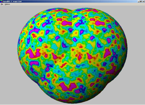
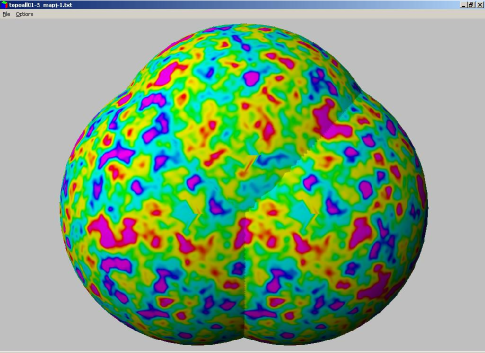
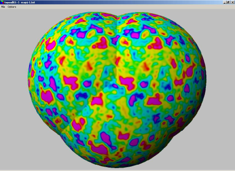
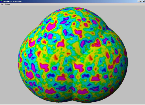
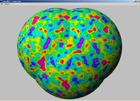
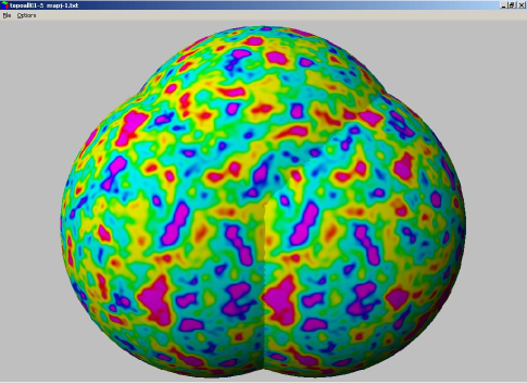
Figure 11: The last scattering surface seen from outside for a Hantzsche-Wendt space $E_{6}$ with $L_{x}=L_{y}=L_{z}=0.64$ in units of the last scattering surface. The geometry of the circle pairings corresponds to the geometry of the fundamental polyhedron. The pairs of matching circles are shown here looking from directions parallel to the $x$-, $y$-, and $z$-axes, respectively. Only the Sachs-Wolfe contribution has been depicted here.

V.2.6 Klein space

Klein space is generated by two glide reflections

$$\left(\begin{array}[]{c}{x}\\ {y}\\ {z}\end{array}\right)\;\mapsto\;\left(\begin{array}[]{rrr}{1}&{0}&{0}\\ {0}&{-1}&{0}\\ {0}&{0}&{\;\;\;1}\end{array}\right)\left(\begin{array}[]{c}{x}\\ {y}\\ {z}\end{array}\right)+\left(\begin{array}[]{c}{L_{x}/2}\\ {L_{y}/2}\\ {0}\end{array}\right),\qquad\left(\begin{array}[]{c}{x}\\ {y}\\ {z}\end{array}\right)\;\mapsto\;\left(\begin{array}[]{rrr}{1}&{0}&{0}\\ {0}&{-1}&{0}\\ {0}&{0}&{\;\;\;1}\end{array}\right)\left(\begin{array}[]{c}{x}\\ {y}\\ {z}\end{array}\right)+\left(\begin{array}[]{c}{L_{x}/2}\\ {-L_{y}/2}\\ {0}\end{array}\right),\qquad$$ (93)

along with a simple translation

$$\left(\begin{array}[]{c}{x}\\ {y}\\ {z}\end{array}\right)\;\mapsto\;\left(\begin{array}[]{c}{x}\\ {y}\\ {z}\end{array}\right)+\left(\begin{array}[]{c}{0}\\ {0}\\ {L_{z}}\end{array}\right).$$ (94)

The first (resp. second) glide reflection corresponds to the two upper (resp. lower) faces of the hexagonal prism in Figure 1, taking one to the other so that the small dark-colored (resp. light-colored) windows match. The simple translation takes the front hexagonal face to the back hexagonal face so that the doors match.

The square of either glide reflection is a horizontal translation ${\bf T}=(L_{x},0,0)$ (taking the unmarked left wall to the unmarked right wall in Figure 1), while the composition of one glide reflection with the inverse of the other is a vertical translation ${\bf T}=(0,L_{y},0)$. Thus the Klein space is the two-fold quotient of a rectangular 3-torus of size $(L_{x},L_{y},L_{z})$.

To find the Klein space’s eigenmodes, we begin with the modes (19) of the rectangular 3-torus and ask which remain invariant under the glide reflections (93). The Invariance Lemma shows the Klein space’s eigenmodes have the orthonormal basis

$$\begin{array}[]{lcl}\frac{1}{\sqrt{2}}\left[\Upsilon_{2\pi(\frac{n_{x}}{L_{x}},\frac{n_{y}}{L_{y}},\frac{n_{z}}{L_{z}})}+(-1)^{n_{x}+n_{y}}\Upsilon_{2\pi(\frac{n_{x}}{L_{x}},-\frac{n_{y}}{L_{y}},\frac{n_{z}}{L_{z}})}\right]&\quad\mbox{for}&n_{y}\in Z^{+},\;n_{x},n_{z}\in Z,\\ \Upsilon_{2\pi(\frac{n_{x}}{L_{x}},0,\frac{n_{z}}{L_{z}})}&\quad\mbox{for}&n_{x}\in 2Z,\;n_{z}\in Z.\\ \end{array}$$ (95)

One can easily check that

$$\Upsilon_{k_{x},k_{y},k_{z}}^{[E_{7}]*}=(-1)^{n_{x}+n_{y}}\Upsilon_{-k_{x},k_{y},-k_{z}}^{[E_{7}]},$$ (96)

when $n_{y}\in Z^{+},\;n_{x},n_{z}\in Z$ and that $\Upsilon_{k_{x},k_{y},k_{z}}^{[E_{7}]}$ is real otherwise. It follows that the analog of Eq. (25) is given by

1. when $n_{y}\in Z^{+},\;n_{x},n_{z}\in Z$, $\hat{e}_{\bf k}$ must satisfy

   $$\hat{e}_{k_{x},k_{y},k_{z}}^{*}=(-1)^{n_{x}+n_{y}}\hat{e}_{-k_{x},k_{y},-k_{z}}.$$ (97)

   It is thus a real random variable when $k_{x}=k_{z}=0$ and $n_{y}\in 2Z$ and a purely imaginary random variable when when $k_{x}=k_{z}=0$ and $n_{y}\notin 2Z$,

2. when $n_{x}\in 2Z$, $n_{y}=0$ and $n_{z}\in Z$, $\hat{e}_{k_{x},0,k_{z}}$ is a real random variable.

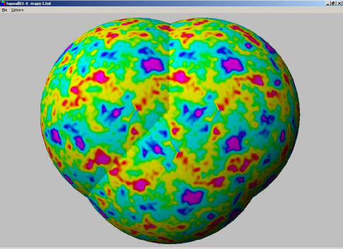
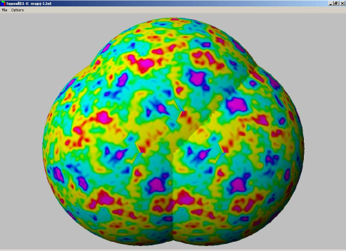
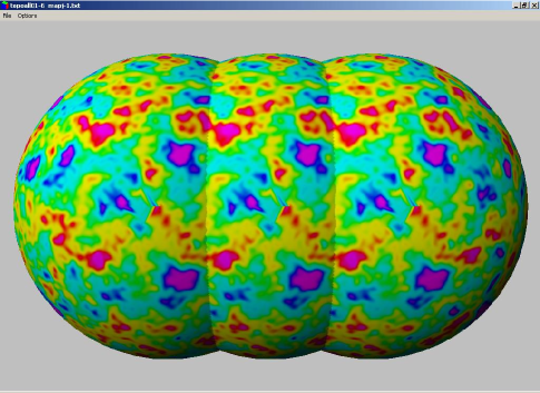
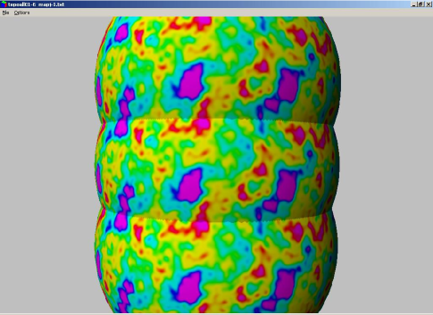
Figure 12: The last scattering surface seen from outside for a Klein space space $E_{7}$ with $L_{x}=L_{y}=L_{z}=0.64$. We present four pairs of matched circles. The lower right figure corresponds to the translation along the $z$ axis while the three other plots corresponds to the holonomies acting in the $xy$-plane. Only the Sachs-Wolfe contribution has been depicted here.

V.2.7 Klein space with horizontal flip

The Klein space with horizontal flip is a two-fold quotient of the plain Klein space. It includes the same two glide reflections (93) as the Klein space, but adds a square root

$$\left(\begin{array}[]{c}{x}\\ {y}\\ {z}\end{array}\right)\;\mapsto\;\left(\begin{array}[]{rrr}{-1}&{0}&{0}\\ {0}&{\;\;\;1}&{0}\\ {0}&{0}&{\;\;\;1}\end{array}\right)\left(\begin{array}[]{c}{x}\\ {y}\\ {z}\end{array}\right)+\left(\begin{array}[]{c}{0}\\ {0}\\ {L_{z}/2}\end{array}\right),$$ (98)

of the Klein space’s $L_{z}$-translation (94). Because the Klein space with horizontal flip is a quotient of the plain Klein space, every eigenmode of the former is automatically an eigenmode of the latter (recall the reasoning of the first paragraph of Section IV). Thus our task is to decide which of the Klein space’s eigenmodes (95) are preserved by the new generator (98). The Invariance Lemma shows the orthonormal basis to be

$$\begin{array}[]{lcl}\frac{1}{2}\left[\Upsilon_{2\pi(\frac{n_{x}}{L_{x}},\frac{n_{y}}{L_{y}},\frac{n_{z}}{L_{z}})}+(-1)^{n_{x}+n_{y}}\Upsilon_{2\pi(\frac{n_{x}}{L_{x}},-\frac{n_{y}}{L_{y}},\frac{n_{z}}{L_{z}})}\right.&&\\ \quad\left.+(-1)^{n_{z}}\Upsilon_{2\pi(-\frac{n_{x}}{L_{x}},\frac{n_{y}}{L_{y}},\frac{n_{z}}{L_{z}})}+(-1)^{n_{x}+n_{y}+n_{z}}\Upsilon_{2\pi(-\frac{n_{x}}{L_{x}},-\frac{n_{y}}{L_{y}},\frac{n_{z}}{L_{z}})}\right]&\quad\mbox{for}&n_{x},n_{y}\in Z^{+},\;n_{z}\in Z,\\ \frac{1}{\sqrt{2}}\left[\Upsilon_{2\pi(0,\frac{n_{y}}{L_{y}},\frac{n_{z}}{L_{z}})}+(-1)^{n_{y}}\Upsilon_{2\pi(0,-\frac{n_{y}}{L_{y}},\frac{n_{z}}{L_{z}})}\right]&\quad\mbox{for}&n_{y}\in Z^{+},\;n_{z}\in 2Z,\\ \frac{1}{\sqrt{2}}\left[\Upsilon_{2\pi(\frac{n_{x}}{L_{x}},0,\frac{n_{z}}{L_{z}})}+(-1)^{n_{z}}\Upsilon_{2\pi(-\frac{n_{x}}{L_{x}},0,\frac{n_{z}}{L_{z}})}\right]&\quad\mbox{for}&n_{x}\in 2Z^{+},\;n_{z}\in Z,\\ \Upsilon_{2\pi(0,0,\frac{n_{z}}{L_{z}})}&\quad\mbox{for}&n_{z}\in 2Z.\\ \end{array}$$ (99)

Following the same procedure as before, we obtain that the analog of Eq. (25) is given by

1. when $n_{x},n_{y}\in Z^{+},\;n_{z}\in Z$, $\hat{e}_{\bf k}$ must satisfy

   $$\hat{e}_{k_{x},k_{y},k_{z}}^{*}=(-1)^{n_{x}+n_{y}+n_{z}}\hat{e}_{k_{x},k_{y},-k_{z}}.$$ (100)

   It is thus a real random variable when $n_{z}=0$ and $n_{x}+n_{y}\in 2Z$ and a purely imaginary random variable when $n_{z}=0$ and $n_{x}+n_{y}\notin 2Z$,

2. when $n_{x}=0$, $n_{y}\in Z^{+}$ and $n_{z}\in Z$, $\hat{e}_{0,k_{y},k_{z}}$ must satisfy

   $$\hat{e}_{0,k_{y},k_{z}}^{*}=(-1)^{n_{y}}\hat{e}_{0,k_{y},-k_{z}},$$ (101)

   so that it is a real random variable when $k_{z}=0$ and $n_{y}\in 2Z$ and a purely imaginary random variable when $n_{z}=0$ and $n_{y}\notin 2Z$,

3. when $n_{x}\in Z^{+}$, $n_{y}=0$ and $n_{z}\in Z$, $\hat{e}_{k_{x},0,k_{z}}$ must satisfy

   $$\hat{e}_{k_{x},0,k_{z}}^{*}=(-1)^{n_{z}}\hat{e}_{k_{x},0,-k_{z}},$$ (102)

   so that it is a real random variable when $k_{z}=0$,

4. when $n_{z}\in 2Z$ it has to satisfy

   $$\hat{e}_{0,0,k_{z}}^{*}=\hat{e}_{0,0,-k_{z}}.$$ (103)

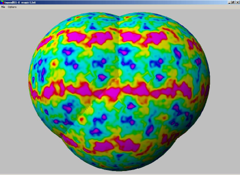
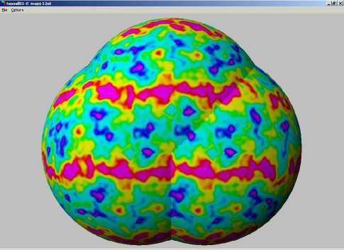
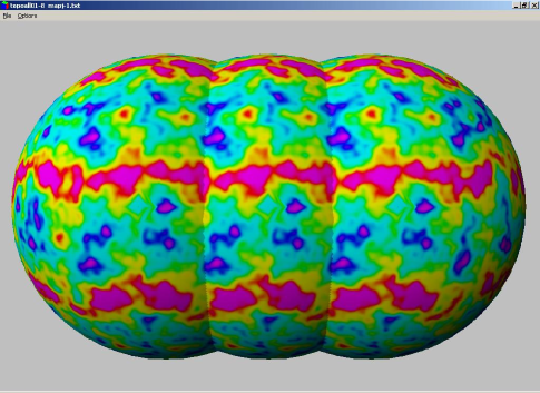
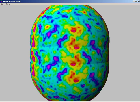
Figure 13: The last scattering surface seen from outside for a Klein space with horizontal flip $E_{8}$ with $L_{x}=L_{y}=L_{z}=0.64$. We present four pairs of matched circles. The first three are identical to those of Klein space, while the last one corresponds to the transformation along the $z$-axis (the upper and lower circles are mirror images of each other). Only the Sachs-Wolfe contribution has been depicted here.

V.2.8 Klein space with vertical flip

The Klein space with vertical flip replaces (98) with

$$\left(\begin{array}[]{c}{x}\\ {y}\\ {z}\end{array}\right)\;\mapsto\;\left(\begin{array}[]{rrr}{1}&{0}&{0}\\ {0}&{-1}&{0}\\ {0}&{0}&{\;\;\;1}\end{array}\right)\left(\begin{array}[]{c}{x}\\ {y}\\ {z}\end{array}\right)+\left(\begin{array}[]{c}{0}\\ {0}\\ {L_{z}/2}\end{array}\right),$$ (104)

whose action interchanges the modes $\Upsilon_{(k_{x},k_{y},k_{z})}\leftrightarrow(-1)^{n_{z}}\Upsilon_{(k_{x},-k_{y},k_{z})}$. Consistency with the glide reflections (93), whose action interchanges $\Upsilon_{(k_{x},k_{y},k_{z})}\leftrightarrow(-1)^{n_{x}+n_{y}}\Upsilon_{(k_{x},-k_{y},k_{z})}$, requires $n_{x}+n_{y}\equiv n_{z}\mbox{ (mod }{2})$. Thus the orthonormal basis is

$$\begin{array}[]{lcl}\frac{1}{\sqrt{2}}\left[\Upsilon_{2\pi(\frac{n_{x}}{L_{x}},\frac{n_{y}}{L_{y}},\frac{n_{z}}{L_{z}})}+(-1)^{n_{x}+n_{y}}\Upsilon_{2\pi(\frac{n_{x}}{L_{x}},-\frac{n_{y}}{L_{y}},\frac{n_{z}}{L_{z}})}\right]&\quad\mbox{for}&n_{y}\in Z^{+},\;n_{x},n_{z}\in Z,\;n_{x}+n_{y}\equiv n_{z}\mbox{ (mod }{2}),\\ \Upsilon_{2\pi(\frac{n_{x}}{L_{x}},0,\frac{n_{z}}{L_{z}})}&\quad\mbox{for}&n_{x},n_{z}\in 2Z.\\ \end{array}$$ (105)

Following the same procedure as before, we obtain that the analog of Eq. (25) is given by

1. when $n_{y}\in Z^{+}$ and $n_{x},n_{z}\in Z$ with $n_{x}+n_{y}\equiv n_{z}\mbox{ (mod }{2})$, $\hat{e}_{\bf k}$ must satisfy

   $$\hat{e}_{k_{x},k_{y},k_{z}}^{*}=(-1)^{n_{z}}\hat{e}_{-k_{x},k_{y},-k_{z}},$$ (106)

   so that it is a real random variable when $k_{x}=k_{z}=0$,

2. when $n_{x},n_{z}\in 2Z$, it has to be such that

   $$\hat{e}_{k_{x},0,k_{z}}^{*}=\hat{e}_{-k_{x},0,-k_{z}}.$$ (107)

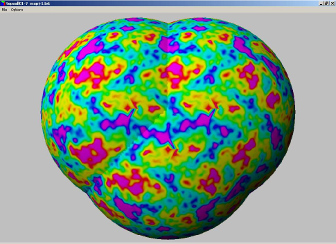
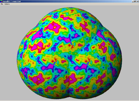
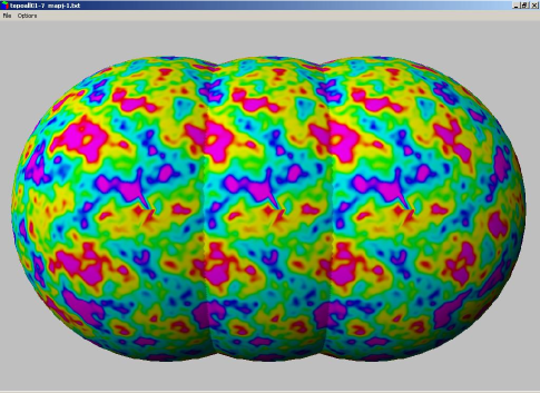
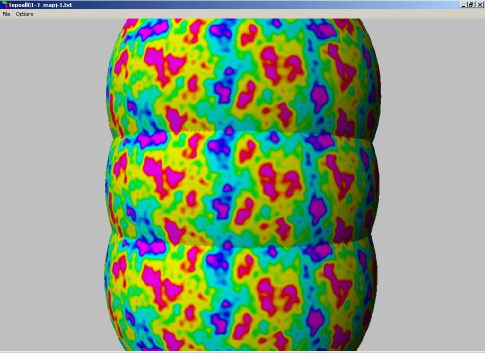
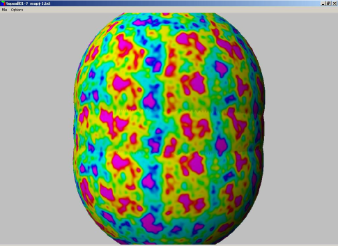
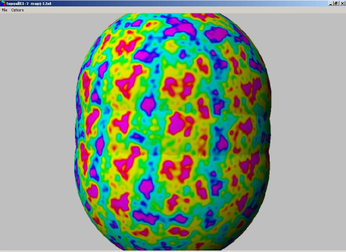
Figure 14: The last scattering surface seen from outside for a Klein space with vertical flip $E_{9}$ with $L_{x}=L_{y}=L_{z}=0.64$. We present the six pairs of matched circles. The first two rows correspond to the same holonomies as for the Klein space, while the last row corresponds to the translation plus flip specific to this space. Two different views of the same holonomy are shown.

V.2.9 Klein space with half turn

The Klein space with half turn replaces (98) or (104) with

$$\left(\begin{array}[]{c}{x}\\ {y}\\ {z}\end{array}\right)\;\mapsto\;\left(\begin{array}[]{rrr}{-1}&{0}&{0}\\ {0}&{-1}&{0}\\ {0}&{0}&{\;\;\;1}\end{array}\right)\left(\begin{array}[]{c}{x}\\ {y}\\ {z}\end{array}\right)+\left(\begin{array}[]{c}{0}\\ {0}\\ {L_{z}/2}\end{array}\right),$$ (108)

The orthonormal eigenbasis, which differs only slightly from that of the Klein space with horizontal flip (99), is

$$\begin{array}[]{lcl}\frac{1}{2}\left[\Upsilon_{2\pi(\frac{n_{x}}{L_{x}},\frac{n_{y}}{L_{y}},\frac{n_{z}}{L_{z}})}+(-1)^{n_{x}+n_{y}}\Upsilon_{2\pi(\frac{n_{x}}{L_{x}},-\frac{n_{y}}{L_{y}},\frac{n_{z}}{L_{z}})}\right.&&\\ \quad\left.+(-1)^{n_{z}}\Upsilon_{2\pi(-\frac{n_{x}}{L_{x}},-\frac{n_{y}}{L_{y}},\frac{n_{z}}{L_{z}})}+(-1)^{n_{x}+n_{y}+n_{z}}\Upsilon_{2\pi(-\frac{n_{x}}{L_{x}},\frac{n_{y}}{L_{y}},\frac{n_{z}}{L_{z}})}\right]&\quad\mbox{for}&n_{x},n_{y}\in Z^{+},\;n_{z}\in Z,\\ \frac{1}{\sqrt{2}}\left[\Upsilon_{2\pi(0,\frac{n_{y}}{L_{y}},\frac{n_{z}}{L_{z}})}+(-1)^{n_{y}}\Upsilon_{2\pi(0,-\frac{n_{y}}{L_{y}},\frac{n_{z}}{L_{z}})}\right]&\quad\mbox{for}&n_{y}\in Z^{+},\;n_{z}\in Z,\;n_{y}\equiv n_{z}\mbox{ (mod }{2}),\\ \frac{1}{\sqrt{2}}\left[\Upsilon_{2\pi(\frac{n_{x}}{L_{x}},0,\frac{n_{z}}{L_{z}})}+(-1)^{n_{z}}\Upsilon_{2\pi(-\frac{n_{x}}{L_{x}},0,\frac{n_{z}}{L_{z}})}\right]&\quad\mbox{for}&n_{x}\in 2Z^{+},\;n_{z}\in Z,\\ \Upsilon_{2\pi(0,0,\frac{n_{z}}{L_{z}})}&\quad\mbox{for}&n_{z}\in 2Z.\\ \end{array}$$ (109)

Following the same procedure as before, we obtain that the analog of Eq. (25) is given by

1. when $n_{x},n_{y}\in Z^{+}$ and $n_{z}\in Z$, $\hat{e}_{\bf k}$ must satisfy

   $$\hat{e}_{k_{x},k_{y},k_{z}}^{*}=(-1)^{n_{z}}\hat{e}_{k_{x},k_{y},-k_{z}},$$ (110)

   so that it is a real random variable when $k_{z}=0$,

2. when $n_{y}\in Z^{+}$, $n_{z}\in Z$ and $n_{y}\equiv n_{z}\mbox{ (mod }{2})$, $\hat{e}_{\bf k}$ must satisfy

   $$\hat{e}_{0,k_{y},k_{z}}^{*}=(-1)^{n_{y}}\hat{e}_{0,k_{y},-k_{z}},$$ (111)

   so that it is a real random variable when $k_{z}=0$ and $n_{y}\in 2Z$ and a purely imaginary random variable when $k_{z}=0$ and $n_{y}\notin 2Z$.

3. when $n_{x}\in 2Z^{+}$ and $n_{z}\in Z$, $\hat{e}_{\bf k}$ must satisfy

   $$\hat{e}_{k_{x},0,k_{z}}^{*}=(-1)^{n_{z}}\hat{e}_{k_{x},0,-k_{z}},$$ (112)

   so that it is a real random variable when $k_{z}=0$

4. when $n_{z}\in 2Z$, it has to be such that

   $$\hat{e}_{0,0,k_{z}}^{*}=\hat{e}_{0,0,-k_{z}}.$$ (113)

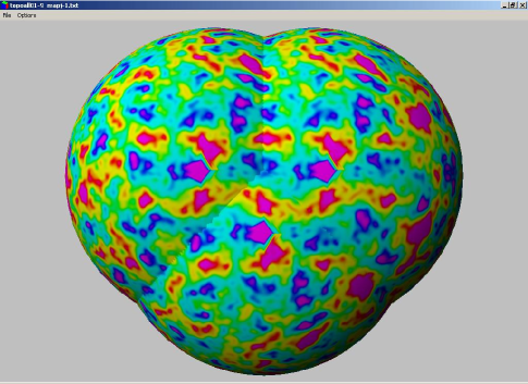
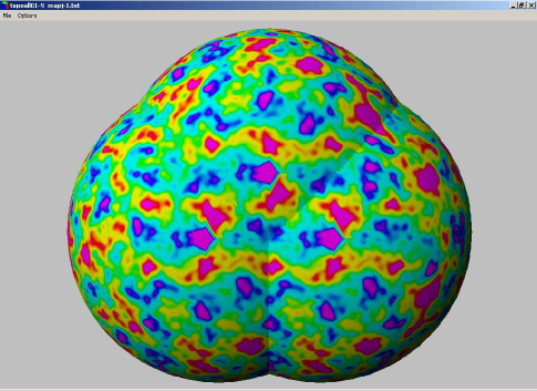
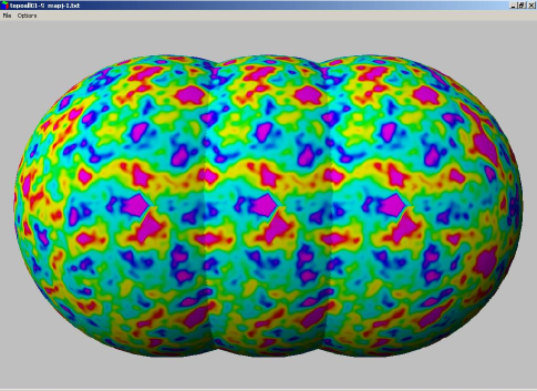
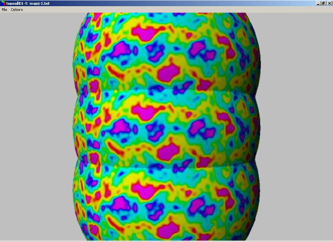
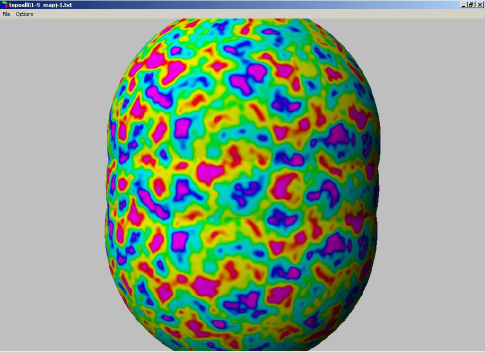
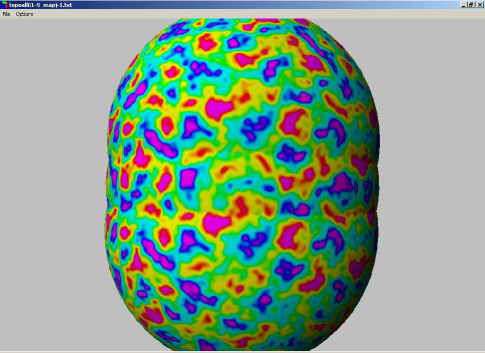
Figure 15: The last scattering surface seen from outside for a Klein space with half turn $E_{10}$ with $L_{x}=L_{y}=L_{z}=0.64$. We present the six pairs of matched circles. The two upper left rows correspond to the same holonomies as for the Klein space, while the last row corresponds to the translation plus half turn holonomy specific to this space. Two different views of the same holonomy are shown.

VI Doubly Periodic Spaces

We will first find the eigenmodes of the chimney space, and then use them to find the eigenmodes of its quotients.

VI.1 Chimney Space

Just as a 3-torus is the quotient of Euclidean space ${{\bf{E}}}^{3}$ under the action of three linearly independent translations ${\bf T}_{1}$, ${\bf T}_{2}$ and ${\bf T}_{3}$, a chimney space is the quotient of ${{\bf{E}}}^{3}$ by only two linearly independent translations ${\bf T}_{1}$ and ${\bf T}_{2}$. Its fundamental domain is an infinitely tall chimney whose cross section is a parallelogram (Figure 2). And just as the allowable wave vectors ${\bf k}$ for an eigenmode $\Upsilon_{\bf k}$ of a 3-torus were defined by the intersection of three families of parallel planes (Section V.1), the allowable wave vectors ${\bf k}$ for an eigenmode $\Upsilon_{\bf k}$ of a chimney space are defined by the intersection of two families of parallel planes. Thus the allowable wave vectors form a latticework of parallel lines.

The most important special case is the rectangular chimney space generated by two orthogonal translations

$${\bf T}_{1} =(L_{x},0,0),$$

$${\bf T}_{2} =(0,L_{y},0),$$ (114)

in which case the allowed wave vectors ${\bf k}$ take the form

$${\bf k}=2\pi\,\left(\frac{n_{x}}{L_{x}},\,\frac{n_{y}}{L_{y}},\,r_{z}\right)$$ (115)

for integer values of $n_{x}$ and $n_{y}$ and real values of $r_{z}$. The corresponding orthonormal basis

$$\begin{array}[]{lcl}\Upsilon_{2\pi(\frac{n_{x}}{L_{x}},\frac{n_{y}}{L_{y}},r_{z})}&\quad\mbox{for}&n_{x},n_{y}\in Z,\;r_{z}\in R\end{array}$$ (116)

is continuous, not discrete as for the 3-torus. Nevertheless, restricting to a fixed modulus $k=|{\bf k}|$ recovers a finite-dimensional basis.

The next four spaces are quotients of the chimney space, so their eigenmodes will form subspaces of those of the chimney space itself.

As in the case of the torus, the random variable $\hat{e}_{\bf k}$ is a complex random variable satisfying

$$\hat{e}_{\bf k}^{*}=\hat{e}_{-{\bf k}}.$$ (117)

VI.2 Quotients of the Chimney Space

VI.2.1 Chimney space with half turn

The chimney space with half turn (Figure 2) is generated by the rectangular chimney space’s $x$-translation ${\bf T}_{1}=(L_{x},0,0)$ along with

$$\left(\begin{array}[]{c}{x}\\ {y}\\ {z}\end{array}\right)\;\mapsto\;\left(\begin{array}[]{rrr}{-1}&{0}&{0}\\ {0}&{\;\;\;1}&{0}\\ {0}&{0}&{-1}\end{array}\right)\left(\begin{array}[]{c}{x}\\ {y}\\ {z}\end{array}\right)+\left(\begin{array}[]{c}{0}\\ {0}\\ {L_{y}/2}\end{array}\right).$$ (118)

Even though the eigenmodes are not discrete, the Invariance Lemma applies exactly as in the compact case, giving the eigenbasis

$$\begin{array}[]{lcl}\frac{1}{\sqrt{2}}\left[\Upsilon_{2\pi(\frac{n_{x}}{L_{x}},\frac{n_{y}}{L_{y}},r_{z})}+(-1)^{n_{y}}\Upsilon_{2\pi(-\frac{n_{x}}{L_{x}},\frac{n_{y}}{L_{y}},-r_{z})}\right]&\quad\mbox{for}&(n_{x}\in Z^{+},r_{z}\in R)\mbox{ or }(n_{x}=0,r_{z}\in R^{+}),\\ \Upsilon_{2\pi(0,\frac{n_{y}}{L_{y}},0)}&\quad\mbox{for}&n_{y}\in 2Z.\\ \end{array}$$ (119)

This case is analogous to the case of the half turn space so the analog of Eq. (25) is given by

1. when $(n_{x}\in Z^{+},r_{z}\in R)$ or $(n_{x}=0,r_{z}\in R^{+})$, $\hat{e}_{\bf k}$ satisfies

   $$\hat{e}_{k_{x},k_{y},k_{z}}^{*}=(-1)^{n_{y}}\hat{e}_{k_{x},-k_{y},k_{z}}.$$ (120)

   It is thus a real random variable when $n_{y}=0$ and complex otherwise,

2. when $n_{y}\in 2Z$, $\hat{e}_{\bf k}$ satisfies

   $$\hat{e}_{0,k_{y},0}^{*}=\hat{e}_{0,-k_{y},0}.$$ (121)

VI.2.2 Chimney space with vertical flip

The chimney space with vertical flip (Figure 2) is generated by the translation ${\bf T}_{1}=(L_{x},0,0)$ along with

$$\left(\begin{array}[]{c}{x}\\ {y}\\ {z}\end{array}\right)\;\mapsto\;\left(\begin{array}[]{rrr}{1}&{0}&{0}\\ {0}&{\;\;\;1}&{0}\\ {0}&{0}&{-1}\end{array}\right)\left(\begin{array}[]{c}{x}\\ {y}\\ {z}\end{array}\right)+\left(\begin{array}[]{c}{0}\\ {L_{y}/2}\\ {0}\end{array}\right).$$ (122)

The Invariance Lemma shows the orthonormal eigenbasis to be

$$\begin{array}[]{lcl}\frac{1}{2}\left[\Upsilon_{2\pi(\frac{n_{x}}{L_{x}},\frac{n_{y}}{L_{y}},r_{z})}+(-1)^{n_{y}}\Upsilon_{2\pi(\frac{n_{x}}{L_{x}},\frac{n_{y}}{L_{y}},-r_{z})}\right]&\quad\mbox{for}&n_{x},n_{y}\in Z,\;r_{z}\in R^{+},\\ \Upsilon_{2\pi(\frac{n_{x}}{L_{x}},\frac{n_{y}}{L_{y}},0)}&\quad\mbox{for}&n_{x}\in Z,\;n_{y}\in 2Z.\\ \end{array}$$ (123)

One might also consider a chimney space with a vertical flip in the $x$-direction as well as the $y$-direction. Surprisingly, such a space turns out to be equivalent to a chimney space with a single flip, but with cross section a parallelogram rather than a rectangle. In other words, the chimney space with two flips has the same topology as the chimney space with one flip, even though they may differ geometrically.

Concerning the properties of the random variable, the analog of Eq. (25) is given by

1. when $n_{x},n_{y}\in Z$ and $r_{z}\in R^{+}$, $\hat{e}_{\bf k}$ satisfies

   $$\hat{e}_{k_{x},k_{y},k_{z}}^{*}=(-1)^{n_{y}}\hat{e}_{-k_{x},-k_{y},k_{z}},$$ (124)

   it is thus a real random variable when $k_{x}=k_{y}=0$,

2. when $n_{x}\in Z$ and $n_{y}\in 2Z$, $\hat{e}_{\bf k}$ satisfies

   $$\hat{e}_{k_{x},k_{y},0}^{*}=\hat{e}_{-k_{x},-k_{y},0}.$$ (125)

VI.2.3 Chimney space with horizontal flip

The chimney space with horizontal flip (Figure 2) is generated by the translation ${\bf T}_{1}=(L_{x},0,0)$ along with

$$\left(\begin{array}[]{c}{x}\\ {y}\\ {z}\end{array}\right)\;\mapsto\;\left(\begin{array}[]{rrr}{-1}&{0}&{0}\\ {0}&{\;\;\;1}&{0}\\ {0}&{0}&{\;\;\;1}\end{array}\right)\left(\begin{array}[]{c}{x}\\ {y}\\ {z}\end{array}\right)+\left(\begin{array}[]{c}{0}\\ {L_{y}/2}\\ {0}\end{array}\right).$$ (126)

The Invariance Lemma shows the orthonormal eigenbasis to be

$$\begin{array}[]{lcl}\frac{1}{\sqrt{2}}\left[\Upsilon_{2\pi(\frac{n_{x}}{L_{x}},\frac{n_{y}}{L_{y}},r_{z})}+(-1)^{n_{y}}\Upsilon_{2\pi(-\frac{n_{x}}{L_{x}},\frac{n_{y}}{L_{y}},r_{z})}\right]&\quad\mbox{for}&n_{x}\in Z^{+},\;n_{y}\in Z,\;r_{z}\in R,\\ \Upsilon_{2\pi(0,\frac{n_{y}}{L_{y}},r_{z})}&\quad\mbox{for}&n_{y}\in 2Z,\;r_{z}\in R.\\ \end{array}$$ (127)

Concerning the properties of the random variable, the analog of Eq. (25) is given by

1. when $n_{x}\in Z$, $n_{y}\in Z$ and $r_{z}\in R$, $\hat{e}_{\bf k}$ satisfies

   $$\hat{e}_{k_{x},k_{y},k_{z}}^{*}=(-1)^{n_{y}}\hat{e}_{k_{x},-k_{y},-k_{z}},$$ (128)

   it is thus a real random variable when $k_{y}=k_{z}=0$,

2. when $n_{y}\in 2Z$ and $r_{z}\in R$, $\hat{e}_{\bf k}$ satisfies

   $$\hat{e}_{0,k_{y},0}^{*}=\hat{e}_{0,-k_{y},0}.$$ (129)

VI.2.4 Chimney space with half turn and flip

The chimney space with half turn and flip (Figure 2) is generated by

$$\left(\begin{array}[]{c}{x}\\ {y}\\ {z}\end{array}\right)\;\mapsto\;\left(\begin{array}[]{rrr}{-1}&{0}&{0}\\ {0}&{\;\;\;1}&{0}\\ {0}&{0}&{-1}\end{array}\right)\left(\begin{array}[]{c}{x}\\ {y}\\ {z}\end{array}\right)+\left(\begin{array}[]{c}{0}\\ {L_{y}/2}\\ {0}\end{array}\right),$$ (130)

and

$$\left(\begin{array}[]{c}{x}\\ {y}\\ {z}\end{array}\right)\;\mapsto\;\left(\begin{array}[]{rrr}{1}&{0}&{0}\\ {0}&{\;\;\;1}&{0}\\ {0}&{0}&{-1}\end{array}\right)\left(\begin{array}[]{c}{x}\\ {y}\\ {z}\end{array}\right)+\left(\begin{array}[]{c}{L_{x}/2}\\ {0}\\ {0}\end{array}\right).$$ (131)

It is a four-fold quotient of the plain chimney space, unlike the preceding examples, which were two-fold quotients. The Invariance Lemma gives an orthonormal basis for its eigenmodes

$$\begin{array}[]{lcl}\frac{1}{2}\left[\Upsilon_{2\pi(\frac{n_{x}}{L_{x}},\frac{n_{y}}{L_{y}},r_{z})}+(-1)^{n_{y}}\Upsilon_{2\pi(-\frac{n_{x}}{L_{x}},\frac{n_{y}}{L_{y}},-r_{z})}\right.&&\\ \quad\left.+(-1)^{n_{x}}\Upsilon_{2\pi(\frac{n_{x}}{L_{x}},\frac{n_{y}}{L_{y}},-r_{z})}+(-1)^{n_{x}+n_{y}}\Upsilon_{2\pi(-\frac{n_{x}}{L_{x}},\frac{n_{y}}{L_{y}},r_{z})}\right]&\quad\mbox{for}&n_{x}\in Z^{+},\;n_{y}\in Z,\;r_{z}\in R^{+},\\ \frac{1}{\sqrt{2}}\left[\Upsilon_{2\pi(0,\frac{n_{y}}{L_{y}},r_{z})}+\Upsilon_{2\pi(0,\frac{n_{y}}{L_{y}},-r_{z})}\right]&\quad\mbox{for}&n_{y}\in 2Z,\;r_{z}\in R^{+},\\ \frac{1}{\sqrt{2}}\left[\Upsilon_{2\pi(\frac{n_{x}}{L_{x}},\frac{n_{y}}{L_{y}},0)}+(-1)^{n_{y}}\Upsilon_{2\pi(-\frac{n_{x}}{L_{x}},\frac{n_{y}}{L_{y}},0)}\right]&\quad\mbox{for}&n_{x}\in 2Z^{+},\;n_{y}\in Z,\\ \Upsilon_{2\pi(0,\frac{n_{y}}{L_{y}},0)}&\quad\mbox{for}&n_{y}\in 2Z.\\ \end{array}$$ (132)

Following the same procedure as before, we obtain that the analog of Eq. (25) is given by

1. when $n_{x}\in Z^{+}$, $n_{y}\in Z$ and $r_{z}\in R^{+}$, $\hat{e}_{\bf k}$ must satisfy

   $$\hat{e}_{k_{x},k_{y},k_{z}}^{*}=(-1)^{n_{y}}\hat{e}_{k_{x},-k_{y},k_{z}},$$ (133)

   so that it is a real random variable when $k_{y}=0$,

2. when $n_{y}\in 2Z$ and $r_{z}\in R^{+}$, $\hat{e}_{\bf k}$ must satisfy

   $$\hat{e}_{0,k_{y},k_{z}}^{*}=\hat{e}_{0,-k_{y},k_{z}},$$ (134)

   so that it is a real random variable when $k_{y}=0$,

3. when $n_{x}\in 2Z^{+}$ and $n_{y}\in Z$, $\hat{e}_{\bf k}$ must satisfy

   $$\hat{e}_{k_{x},0,k_{z}}^{*}=(-1)^{n_{y}}\hat{e}_{k_{x},-k_{y},0},$$ (135)

   so that it is a real random variable when $k_{y}=0$,

4. when $n_{y}\in 2Z$, it has to be such that

   $$\hat{e}_{0,k_{y},0}^{*}=\hat{e}_{0,-k_{y},0}.$$ (136)

VII Singly Periodic Spaces

We will first find the eigenmodes of the slab space, and then use them to find the eigenmodes of the slab space with flip.

VII.1 Slab Space

Just as a 3-torus is the quotient of Euclidean space under the action of three linearly independent translations and a chimney space is the quotient by two translations, a slab space is the quotient of ${{\bf{E}}}^{3}$ by a single translation. Its fundamental domain is an infinitely tall and wide slab (Figure 3), with opposite faces identified straight across. The allowable wave vectors ${\bf k}$ for an eigenmode $\Upsilon_{\bf k}$ of a slab space define a family of parallel planes.

If we choose coordinates so that the translation takes the form

$${\bf T}=(0,0,L_{z}),$$ (137)

then the allowed wave vectors ${\bf k}$ are

$${\bf k}=2\pi\,\left(r_{x},\,r_{y},\,\frac{n_{z}}{L_{z}}\right),$$ (138)

for real values of $r_{x}$ and $r_{y}$ and integer values of $n_{z}$. The corresponding orthonormal basis is

$$\begin{array}[]{lcl}\Upsilon_{2\pi\,(r_{x},\,r_{y},\,\frac{n_{z}}{L_{z}})}&\quad\mbox{for}&r_{x},r_{y}\in R,\;n_{z}\in Z.\end{array}$$ (139)

Even if we restrict to a fixed modulus $k=|{\bf k}|$, the eigenmodes of slab space remain continuous, not discrete.

If desired, one could construct a more general slab space by identifying opposite faces with a rotation. Such a space would be topologically the same as a standard slab space, but geometrically different.

As in the case of the torus and of the chimney space, the random variable $\hat{e}_{\bf k}$ is a complex random variable satisfying

$$\hat{e}_{\bf k}^{*}=\hat{e}_{-{\bf k}}.$$ (140)

VII.2 Slab Space with Flip

A slab space with flip is generated by

$$\left(\begin{array}[]{c}{x}\\ {y}\\ {z}\end{array}\right)\;\mapsto\;\left(\begin{array}[]{rrr}{-1}&{0}&{0}\\ {0}&{\;\;\;1}&{0}\\ {0}&{0}&{\;\;\;1}\end{array}\right)\left(\begin{array}[]{c}{x}\\ {y}\\ {z}\end{array}\right)+\left(\begin{array}[]{c}{0}\\ {0}\\ {L_{z}/2}\end{array}\right).$$ (141)

The Invariance Lemma provides the orthonormal basis for its eigenmodes

$$\begin{array}[]{lcl}\left[\Upsilon_{2\pi\,(r_{x},\,r_{y},\,\frac{n_{z}}{L_{z}})}+(-1)^{n_{z}}\Upsilon_{2\pi\,(-r_{x},\,r_{y},\,\frac{n_{z}}{L_{z}})}\right]&\quad\mbox{for}&r_{x}\in R^{+},\;r_{y}\in R,\;n_{z}\in Z,\\ \Upsilon_{2\pi\,(0,\,r_{y},\,\frac{n_{z}}{L_{z}})}&\quad\mbox{for}&r_{y}\in R,\;n_{z}\in 2Z.\end{array}$$ (142)

Concerning the properties of the random variable, the analog of Eq. (25) is given by

1. when $r_{x}\in R^{+}$, $r_{y}\in R$ and $n_{z}\in Z$, $\hat{e}_{\bf k}$ satisfies

   $$\hat{e}_{k_{x},k_{y},k_{z}}^{*}=(-1)^{n_{z}}\hat{e}_{k_{x},-k_{y},-k_{z}}.$$ (143)

   It is thus a real random variable when $k_{y}=k_{z}=0$,

2. when $r_{y}\in R$ and $n_{z}\in 2Z$, $\hat{e}_{\bf k}$ satisfies

   $$\hat{e}_{0,k_{y},k_{z}}^{*}=\hat{e}_{0,-k_{y},-k_{z}}.$$ (144)

VIII Numerical simulations

We can now compute the correlation matrix and simulate CMB maps for the 17 multi-connected spaces described in the previous sections.

In all the simulations, we have considered a flat $\Lambda$CDM model with $\Omega_{\Lambda}=0.7$, a Hubble parameter $H_{0}\equiv 100h\,{\mbox{km}}\,{\mbox{s}^{-1}}\,{\mbox{Mpc}^{-1}}$ with $h=0.62$, a baryon density $\omega_{\rm b}\equiv\Omega_{\rm b}h^{2}=0.019$ and a spectral index $n_{\scriptscriptstyle{\rm S}}=1$. With this the radius of the last scattering surface is $R_{\rm LSS}=15.0\,{\mbox{Gpc}}$.

We present a series of CMB maps with a resolution of $\ell=120$ for the different spaces. These maps are represented on a sphere portraying the last scattering surface seen from outside in the universal cover. Images of the last scattering surface under the action of a holonomy and its inverse are shown and their intersection gives a pair of matched circles. All the plots presented here contain only the Sachs-Wolfe contribution and omit both the Doppler and integrated Sachs-Wolfe contributions.

For the compact spaces, the characteristics of the fundamental polyhedra are

• $L_{x}=L_{y}=0.64$ for all spaces,

• $L_{z}=1.28$ for the half- and quarter-turn spaces (Figs. 7, 8)

• $L_{z}=1.92$ for the third- and sixth-turn spaces (Figs. 9 and 10)

• $L_{z}=0.64$ for the Hantzsche-Wendt and Klein spaces (Figs. 11 through 15).

Turning to the $C_{\ell}$, let us examine the effects of the topology and of the volume of the fundamental domain.

To understand the properties of the angular power spectrum on large scales, let us develop a simple geometrical argument based on the properties of the eigenmodes of the Laplacian operator (see Ref. [21] for an analogous discussion and Ref. [10] for the spherical case). In the simply connected Euclidean space ${{\bf{E}}}^{3}$, the number $N_{\scriptscriptstyle{\rm SC}}$ of modes between $k$ and $k+\Delta k$ is simply given by $N_{\scriptscriptstyle{\rm SC}}(k)=4\pi k^{2}\Delta k$, whatever the scale. Now, due to the topology, most modes will disappear from the spectrum and we are left with wavenumbers of modulus

$$k=2\pi\sqrt{\left(\frac{n_{x}}{L_{x}}\right)^{2}+\left(\frac{n_{y}}{L_{y}}\right)^{2}+\left(\frac{n_{z}}{L_{z}}\right)^{2}}.$$ (145)

On very small scales (large $k$), the Weyl formula [8] allows us to determine the number $N_{\scriptscriptstyle{\rm MC}}$ of modes remaining in the spectrum: asymptotically, $N_{\scriptscriptstyle{\rm MC}}(<k)\sim Vk^{3}/6\pi^{2}$ (see, e.g., Fig. 2 of Ref. [1]). It follows that the number of modes between $k$ and $k+\Delta k$ is now given by $N_{{\scriptscriptstyle{\rm MC}},\infty}(k)\sim Vk^{2}\Delta k/2\pi^{2}\sim VN_{\scriptscriptstyle{\rm SC}}/(2\pi)^{3}$. Thus we may set the overall normalization on small scales where the effect of the topology reduces to an overall rescaling. But this has implications concerning the large scales.

Consider a rectangular torus with a square cross section of size $L_{x}=L_{y}$ and with height $L_{z}$, and let the relative proportions of $L_{x}$ and $L_{z}$ vary.

When $L_{x}\gg L_{z}$, the space looks like a slab space and the modes on large scales (i.e., such that $2\pi/L_{x}\ll k\ll 2\pi/L_{z}$) have a modulus $k\sim\frac{2\pi}{L_{x}}\sqrt{n_{x}^{2}+n_{y}^{2}}$, so that they approach a two-dimensional distribution. Since the number of modes with $k<k_{0}$ is given by $N(<k_{0})=\sum_{n=0}^{k_{0}^{2}}r_{2}(n)=\pi k_{0}^{2}+{\cal O}(k_{0})$, where $r_{n}(p)$ is the number of representations of $p$ by $n$ squares, allowing zeros and distinguishing signs and order (e.g., $r_{2}(5)=8$ and $r_{3}(4)=6$), we obtain that the number of modes between $k$ and $k+\Delta k$ is now given by $N_{{\scriptscriptstyle{\rm MC}},0}(k)\sim L_{x}^{2}k\Delta k/2\pi$. Defining the relative weight as

$$w(k)\equiv\frac{(2\pi)^{3}}{V}\frac{N_{{\scriptscriptstyle{\rm MC}},0}(k)}{N_{\scriptscriptstyle{\rm SC}}(k)},$$ (146)

we obtain that $w\sim(\pi/kL_{z})\gg 1$ so that the large scale modes are boosted compared with the mode distribution of the simply connected space exactly as if the spectral index $n_{\scriptscriptstyle{\rm S}}$ were lowered by 1. In the hypothesis of a scale invariant spectrum $n_{\scriptscriptstyle{\rm S}}=1$, one therefore expects that the $\ell(\ell+1)C_{\ell}$ spectrum will behave as $\ell^{-1}$ for the relevant scales

When $L_{x}\ll L_{z}$, the space looks like a chimney space and the modes on large scales (i.e., such that $2\pi/L_{z}\ll k\ll 2\pi/L_{x}$) have a modulus $k\sim 2\pi n_{z}/L_{z}$ so that they approach a one-dimensional distribution. It follows that the number of modes between $k$ and $k+\Delta k$ is now given by $N_{{\scriptscriptstyle{\rm MC}},0}(k)\sim L_{z}\Delta k/\pi$, so that $w(k)\sim(2\pi/k^{2}L_{x}^{2})\gg 1$. Again, this will imply a relative boost of the spectrum on large scales as if the spectral index were lowered by 2.

When $L_{x}\sim L_{z}$, as long as we are above the mode cut-off, one has a three-dimensional distribution of modes so that the relative weight of large scale modes is $w\sim 1$, as in a simply connected space. The signature of the topology in the $C_{\ell}$ exists at sufficiently large scales in the form of small spikes around the expected value in a simply connected space due to the discrete nature of the $k$-spectrum.

These results are summarized in Fig. 16.

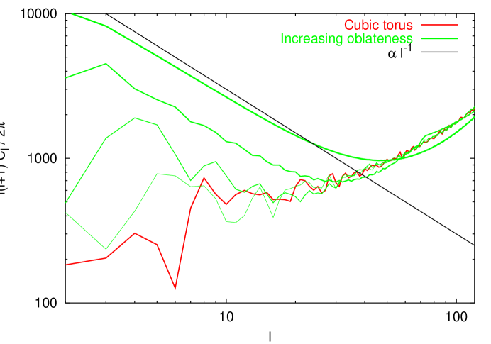
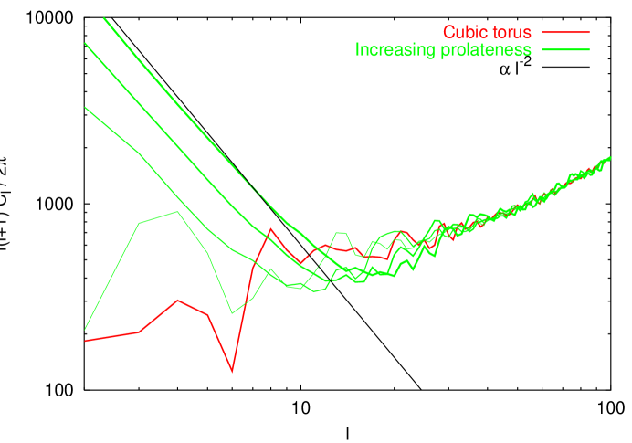
Figure 16: CMB anisotropies in a rectangular torus with $L_{x}=L_{y}$ and $L_{z}<L_{x}$ (left) of $L_{z}>L_{x}$ (right). The volume of the fundamental domain is always the same ($0.262R_{\rm LSS}^{3}$). The spectra start from a cubic torus and $L_{z}$ varies by a factor $2$ from each spectrum to the next (so that the ratio $L_{z}/L_{x}$ reaches $64^{\pm 1}$ for the most anisotropic configurations showed here. The spectrum is boosted and behaves as $\ell^{-1}$ of $\ell^{-2}$ depending on whether the fundamental domain is flattened or elongated along the $z$ direction. Note that the scale at which the cutoff in the spectrum occurs increases with $\max(L_{x},L_{z})$ and that the spikes in the spectrum are less present for large $L_{z}$. This is because the mode spacing decays as $\min(L_{x}^{-1},L_{z}^{-1})$ and hence the discreteness of the spectrum is less obvious. This is of course all the more true when there are two large directions where the mode density is higher (left panel).

IX Location of the Observer

The 3-torus, chimney space, and slab space are exceptional because they are globally homogeneous. A globally homogeneous space looks the same to all observers within it; that is, a global isometry will take any point to any other point. The remaining multi-connected flat spaces, by contrast, are not globally homogeneous and may look different to different observers. For ease of illustration, consider the two-dimensional Klein bottle: the self-intersections of the “last scattering circle” are different for an observer sitting on an axis of glide symmetry (Figure 17 left) than for an observer sitting elsewhere (Figure 17 right). Analogously in three dimensions, the lattice of images of the last scattering surface may differ tremendously for observers sitting at different locations within the same space. The power spectrum, the statistical anisotropies, and the matching circles may all differ.

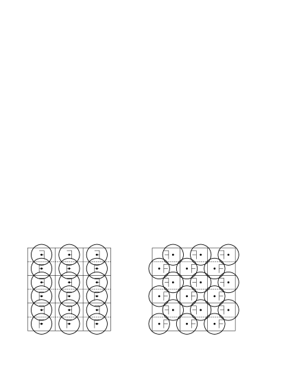
Figure 17: The repeating images of the last scattering circle in a two-dimensional Klein bottle align in rows if the observer happens to sit on an axis of glide symmetry (left), but form a different pattern if the observer sits elsewhere (right).

Moving the observer to a new basepoint would needlessly complicate existing computer software for simulating CMB maps. It is much easier to move the whole universe, leaving the observer fixed! In technical terms, we want to replace an eigenmode $\Upsilon_{\bf k}({\bf x})$ with the translated mode $\Upsilon_{\bf k}({\bf x}+{\bf x}_{\rm obs})$, where ${\bf x}_{\rm obs}$ is the desired location for the observer. The translated mode is quite easy to compute:

$$\Upsilon_{\bf k}({\bf x}) \mapsto \Upsilon_{\bf k}({\bf x}+{\bf x}_{\rm obs})$$ (147)

$$= {\rm e}^{i{\bf k}\cdot({\bf x}+{\bf x}_{\rm obs})}$$

$$= {\rm e}^{i{\bf k}\cdot{\bf x}_{\rm obs}}\;{\rm e}^{i{\bf k}{\bf x}}$$

$$= {\rm e}^{i{\bf k}\cdot{\bf x}_{\rm obs}}\;\Upsilon_{{\bf k}}({\bf x}).$$

For a simple mode $\Upsilon_{\bf k}({\bf x})$, the translation produces a phase shift (by a factor of ${\rm e}^{i{\bf k}\cdot{\bf x}_{\rm obs}}$) and nothing more. The full effect is seen when one considers linear combinations of simple modes:

$$a_{1}\Upsilon_{{\bf k}_{1}}({\bf x})+a_{2}\Upsilon_{{\bf k}_{2}}({\bf x})\quad\mapsto\quad a_{1}{\rm e}^{i{\bf k}_{1}\cdot{\bf x}_{\rm obs}}\Upsilon_{{\bf k}_{1}}({\bf x})+a_{2}{\rm e}^{i{\bf k}_{2}\cdot{\bf x}_{\rm obs}}\Upsilon_{{\bf k}_{2}}({\bf x}).$$ (148)

Each term undergoes a different phase shift, so the final sum may be qualitatively different from the original.

Note that the phase shift (148) induced by the change of the position of the observer does not influence the properties of the statistical variable $\hat{e}_{\bf k}$, but does influence the way a given mode contributes to a given angular scale. This is depicted in Figure 18, where the angular power spectrum is shown in a half-turn space for various positions of the observer. Corresponding examples of maps are shown in Fig. 19.

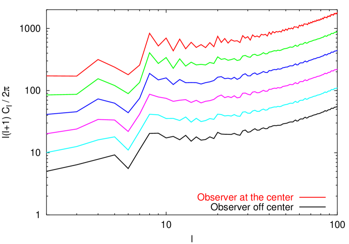
Figure 18: CMB anisotropies in a half-turn space with $L_{x}=L_{y}=0.64$, $L_{z}=1.28$ for various positions of the observer. The observer starts from the center of the fundamental domain and moves along the $x$ axis. As the position and size of some of the matching circles vary, the isotropic part of the angular spectrum also varies. The global structure of the spectrum remains unchanged, but the local “spikes” in the spectrum which originate from the discrete nature of the $k$-spectrum are more or less smoothed depending on the position of the observer. For a better visibility, each spectrum has been offset by a factor of 2 relative to the preceding one (vertical units are arbitrary).

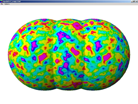
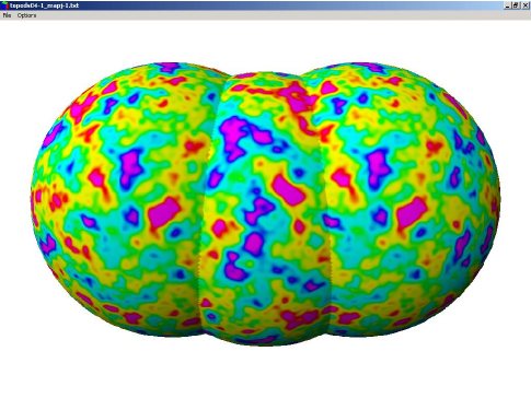
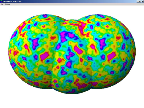
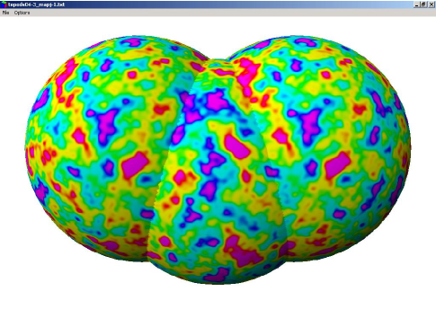
Figure 19: The last scattering surface seen from outside for a half-turn space $E_{2}$ with $L_{x}=L_{y}=0.64$, $L_{z}=1.28$ as in Fig. 7. The observer starts from position $(0,0,0)$, and slowly moves in the $x$ direction. Due to the non-homogeneity of the space, the CMB maps look different.

X Conclusions

This article has presented the tools required to compute CMB maps for all multi-connected flat spaces. We gave for each space

• the polyhedron and holonomy group,

• the eigenmodes of the Laplacian.

We then presented simulated maps for all of the nine compact non homogeneous spaces. On the basis of the angular power spectra we compared the effect of different topologies and different configurations for a given topology. We also implemented the effect of an arbitrary position of the observer which yields significant effects for non-homogeneous spaces. We investigated this effect both on simulated maps and angular power spectra. In particular, it shows that generically matched circles are not back-to-back and that their relative position depends on the position of the observer.

All these tools and simulations will be of great help for extending the conclusions reached on the torus and to investigate their genericity as well as for providing test maps for any method wishing to detect (an interpret) the breakdown of global isotropy.

References

- [1] A. Riazuelo, J.-P. Uzan, R. Lehoucq, and J.W. Weeks, to appear in Phys. Rev. D[arXiv:astro-ph/0212223]; J.-P. Uzan and A. Riazuelo, C. R. Acad. Sci. (Paris), to appear.
- [2] A. Benoît et al., A. & A. 399, L19 (2003); A. Benoît et al., A. & A. 399, L25 (2003).
- [3] D. Spergel et al., Astrophys. J. Suppl. 148, 175 (2003).
- [4] WMAP homepage: [http://map.gsfc.nasa.gov/ ].
- [5] Planck homepage: [http://astro.estec.esa.nl/Planck/ ].
- [6] J. Weeks, R. Lehoucq, and J.-P. Uzan, Class. Quant. Grav. 20, 1529 (2003).
- [7] E. Gausmann, R. Lehoucq, J.-P. Luminet, J.-P. Uzan, and J. Weeks, Class. Quant. Grav. 18, 5155 (2001).
- [8] R. Lehoucq, J. Weeks, J.-P. Uzan, E. Gausmann, and J.-P. Luminet, Class. Quant. Grav. 19 4683, (2002).
- [9] R. Lehoucq, J.-P. Uzan, and J. Weeks, Kodai Math. Journal 26 (2003) 119.
- [10] J.-P. Uzan, A. Riazuelo, R. Lehoucq, and J. Weeks, to appear in Phys. Rev. D[arXiv:astro-ph/0303580].
- [11] J.-P. Luminet, J. Weeks, A. Riazuelo, R. Lehoucq, and J.-P. Uzan, Nature (London) 425 (2003) 593.
- [12] I.Y. Sokolov, JETP Lett. 57, 617 (1993).
- [13] A.A. Starobinsky, JETP Lett. 57, 622 (1993).
- [14] D. Stevens, D. Scott, and J. Silk, Phys. Rev. Lett. 71, 20 (1993).
- [15] A. de Oliveira-Costa and G.F. Smoot, Astrophys. J. 448, 447 (1995).
- [16] J. Levin, E. Scannapieco, G. de Gasperis, and J. Silk, Phys. Rev. D58, 123006 (1998).
- [17] E. Scannapieco, J. Levin, and J. Silk, Month. Not. R. Astron. Soc. 303, 797 (1999).
- [18] R. Bowen and P. Ferreira, Phys. Rev. D66, 04132 (2002).
- [19] K.T. Inoue, Phys. Rev. D62, 103001 (2000).
- [20] K.T. Inoue, Class. Quant. Grav. 18, 1967 (2001).
- [21] K.T. Inoue and N. Sugiyama, Phys. Rev. D67 (2003) 043003.
- [22] B. Roukema, Month. Not. R. Astron. Soc. 312, 712 (2000); ibid. Class. Quant. Grav. 17, 3951 (2000).
- [23] M. Lachièze-Rey and J.-P. Luminet, Phys. Rept. 254 135, (1995).
- [24] J.-P. Uzan, R. Lehoucq, and J.-P. Luminet, in XIXth Texas Symposium on Relativistic Astrophysics and Cosmology, edited by E. Aubourg et al. (Tellig, Châtillon, France), CD-ROM file 04/25.
- [25] J. Levin, Phys. Rept. 365, 251 (2002).
- [26] M. Tegmark, A. de Oliveira-Costa, and A. Hamilton, [arXiv:astro-ph/0302496].
- [27] J.-P. Uzan, U. Kirchner, and G.F.R. Ellis, Month. Not. R. Astron. Soc. 344, L65 (2003); G. Efstathiou, Month. Not. R. Astron. Soc. 343, L95 (2003); C.R. Contaldi, M. Peloso, L. Kofman, and A. Linde, JCAP 0307, 002 (2003); J.M. Cline, P. Crotty, and J. Lesgourgues, JCAP 0309, 010 (2003).
- [28] A. de Oliveira-Costa, M. Tegmark, M. Zaldarriaga, and A. Hamilton, [arXiv:astro-ph/0307282].
- [29] N.J. Cornish, D. Spergel, and G. Starkmann, Class. Quant. Grav. 15, 2657 (1998).
- [30] N. Cornish, D. Spergel, G. Starkman, E. Komatsu, [arXiv:astro-ph/0310233].
- [31] C.J. Copi, D. Huterer, and G.D. Starkman, [arXiv:astro-ph/0310511].
- [32] H.K. Eriksen, F.K. Hansen, A.J. Banday, K.M. Gorski, and P.B. Lilje, [arXiv:astro-ph/0307507].
- [33] C.-G. Park, [arXiv:astro-ph/0307469].
- [34] N.J. Cornish and D.N. Spergel, [arXiv:math.DG/9906017].
- [35] E. Feodoroff, Russian Journ. for Crystallography and mineralogy 21 (1885) 1.
- [36] L. Bierberbach, Mathematische Annalen 70, (1911) 297; Ibid, 72 (1912) 400.
- [37] W. Novacki, Commentarii Mathematici Helvetici 7 (1934) 81.
- [38] C. Adams and J. Shapiro, American Scientist 89, 443 (2001).
- [39] Barry Cipra, What’s Happening in the Mathematical Sciences, Amer. Math. Soc. (2002).
- [40] D.A. Varshalovich, A.N. Moskalev, and V.K. Khersonskii, Quantum theory of angular momentum (World Scientific, Singapore, 1988).