Analyze This! A cosmological constraint package for cmbeasy

Abstract

We introduce a Markov Chain Monte Carlo simulation and data analysis package that extends the Cmbeasy software. We have taken special care in implementing an adaptive step algorithm for the Markov Chain Monte Carlo in order to improve convergence. Data analysis routines are provided which allow to test models of the Universe against measurements of the cosmic microwave background, supernovae Ia and large scale structure. We present constraints on cosmological parameters derived from these measurements for a $\Lambda$CDM cosmology and discuss the impact of the different observational data sets on the parameters. The package is publicly available as part of the Cmbeasy software at www.cmbeasy.org.

1 Introduction

The wealth of recent precision measurements in cosmology [1, 2, 3, 4, 5, 6, 7, 8, 9, 10, 11, 12, 13, 14, 15] places stringent constraints on any model of the Universe. Typically, such a model is given in terms of a number of cosmological parameters. Numerical tools, such as Cmbfast [16], Camb [17] and Cmbeasy [18], permit to calculate the prediction of a given model for the observational data. While these tools are comparatively fast, scanning the parameter space for the most likely model and confidence regions can become a matter of time and computing power.

The cost of evaluating models on a n-dimensional grid in parameter space increases exponentially with the number of parameters. In contrast, the Markov Chain Monte Carlo (MCMC) method scales roughly linearly with the number of parameters [19, 20, 21]. The MCMC method has already been used to constrain various models [22, 24, 25, 23]. A popular tool for setting up MCMC simulations is the Cosmo-Mc package [21] for the Camb code, an improved proposal distribution for the local Metropolis algorithm has been proposed in [26].

In this paper, we introduce the AnalyzeThis package for Cmbeasy. It includes a parallel MCMC driver, as well as routines to calculate the likelihood of a model with respect to various data sets. We took special care in designing a step-proposal strategy that leads to fast convergence and mixing of the chains. This strategy is applied during the early stages of the simulation. As soon as the likelihood contour has been roughly explored, the adaptive step proposal freezes in. This ensures that the MCMC results are not contaminated by the adaptive steps. At the same time, the automated step optimization considerably improves performance and is rather convenient. The raw data files can be processed from within a graphical user interface (gui). Using the gui, one can marginalize, visualize and print one and two dimensional likelihood surfaces (see figure 1).

The plan of this paper is as follows: we describe the MCMC method and our implementation in section 2. A brief introduction to the software is given in section 3. We analyze the constraints on cosmological parameters from observational data sets in section 4. In section 5 we present our conclusions, while the format of the MCMC data files is defined in A.

2 Markov Chain Monte Carlo simulation

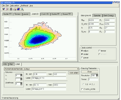
Figure 1: The graphical user interface of Cmbeasy. It can be used to marginalize, visualize and print the one and two dimensional likelihoods from the MCMC chains. Shown is the marginalized likelihood in the $\Omega_{m}h^{2}-\Omega_{b}h^{2}$ plane of a $\Lambda$CDM model.

In the following, we will review the basic ideas of Markov Chain Monte Carlo simulation [27, 28, 29] and describe our implementation.

Suppose that $\theta$ denotes a vector of all model parameters, $X$ represents some observed data and $L(X|\theta)$ is the likelihood of observing $X$ given parameters $\theta$. Specifying a prior distribution $P(\theta)$ for the parameters, Bayes’ theorem yields the posterior distribution $\pi(\theta|X)$ of $\theta$ given the observed data $X$:

$$\pi(\theta|X)=\frac{P(\theta)L(X|\theta)}{\int P(\theta)L(X|\theta)d\theta}.$$ (1)

Using $\pi(\theta|X)$, one can compute expectation values

$$E[f(\theta)|X]=\frac{\int f(\theta)\pi(\theta|X)d\theta}{\int\pi(\theta|X)d\theta},$$ (2)

as well as confidence levels.

The idea of the MCMC method is to directly draw samples from the posterior $\pi(\theta|X)$. The statistical properties of $\pi(\theta|X)$ may then be estimated using this sample. To accomplish the sampling of $\pi(\theta|X)$ one uses a Markov Chain, which is a stochastic process $\{\theta_{0},\theta_{1},...,\theta_{n}\}$ where $\theta_{n}$ only depends on $\theta_{n-1}$. The idea is to choose the next point in the chain based on the previous point such that $\pi(\theta|X)$ becomes the stationary distribution of the chain

$$\mbox{Dist}\{\theta_{0},...,\theta_{n}\}\rightarrow\pi(\theta|X)\mbox{ as }n\rightarrow\infty.$$ (4)

There are several methods to accomplish this. We will concentrate on the Metropolis algorithm [30] and its implementation in Cmbeasy.

2.1 The Metropolis Algorithm

The algorithm is defined as follows (for an illustration see Fig. 2):

1. Choose starting parameter vector $\theta_{0}$.

2. Compute the likelihood $L_{0}(X|\theta_{0})$ of observing the experimental data given the parameters $\theta_{0}$.

3. Obtain a new parameter vector by sampling from a “proposal distribution” $q(\theta_{i-1},\theta_{i})$ (see section 2.3).

4. Compute the likelihood $L_{i}(X|\theta_{i})$.

5. If $L_{i}>L_{i-1}$ then save $\theta_{i}$ as new point in the chain (“take the step”) and go to (3).

6. If $L_{i}<L_{i-1}$ then generate a random variable $u$ from $[0,1]$. If $u<L_{i}/L_{i-1}$ take the step as in (5). If $u>L_{i}/L_{i-1}$ then reject $\theta_{i}$, save $\theta_{i-1}$ as new point in the chain and go to (3).

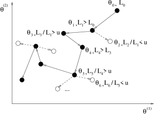
Figure 2: Illustrating the Metropolis algorithm for two parameters. Filled circles represent points belonging to the chain, empty circles are proposed but rejected points not belonging to the chain. In this example, the chain would be $[\theta_{0},\theta_{1},\theta_{1},\theta_{3},\theta_{4},\dots]$.

This algorithm assumes flat priors $P(\theta)$ and a symmetric proposal distribution $q(\theta_{i-1},\theta_{i})=q(\theta_{i},\theta_{i-1})$. Note that we assign likelihood zero to any parameter set that has at least one point outside its prior. In this version of the Metropolis algorithm, all parameters change with every step, a strategy called global Metropolis.

2.2 Convergence Testing

At the beginning, the chain migrates from its random starting point to regions of higher likelihood. Points during this “burn-in” do not constitute a sample from $\pi(\theta|X)$ and should be eliminated. In principle, it may be difficult to tell from a single chain if it has converged towards the underlying $\pi(\theta|X)$. In MCMC, one therefore uses several chains with random starting points and monitors mixing and convergence.

The convergence test of Gelman and Rubin [31] monitors the variance of a parameter between the chains. To be precise, consider using the last $n$ points of each of $m$ chains for the test. Let $\psi_{ij}$ label one entry of the parameter vector $\theta$ at point $j=1,\dots,n$ in chain $i$ with $\overline{\psi}_{i}$ the mean for chain $i$ and $\overline{\psi}$ the mean of all chains. The variance between chains $B$ and the within-chain variance $W$ are then given by

$$B = \frac{n}{m-1}\sum_{i=1}^{m}(\overline{\psi}_{i}-\overline{\psi})^{2},$$ (5)

$$W = \frac{1}{m}\sum_{i=1}^{m}s_{i}^{2},\mbox{ where }s_{i}^{2}=\frac{1}{n-1}\sum_{j=1}^{n}(\psi_{ij}-\overline{\psi}_{i})^{2},$$ (6)

and the quantity

$$R=\frac{\frac{n-1}{n}W+\frac{1}{n}B}{W}$$ (7)

should converge to one. A value of $R<1.2$ for all parameters indicates that the chain is sampling from $\pi(\theta|X)$. From this point onwards one may use the chain points for parameter estimates.

When do we have enough points for parameter estimation? This question is not easy to answer, since it is depends on the model, the used data sets and the desired accuracy how many chain points are needed for a robust estimate of parameters. Therefore, in our implementation the MCMC simulation runs indefinetly. However, any “breaking-criterion” may be implemented easily, and the chains may be monitored with external programs during the run.

2.3 Adaptive Step Size Gaussian Sampler

The number of steps needed for good convergence and mixing depends strongly on the step proposal distribution. If the proposed steps are too large, the algorithm will frequently reject steps, giving slow convergence of the chain. If, on the other hand, the proposed steps are too small, it will take a long time for the chain to explore the likelihood surface, resulting in slow mixing. In the ideal case the proposal distribution should be as close to the posterior distribution $\pi(\theta|X)$ as possible – which unfortunately is not known a priori. While a simple Gaussian proposal distribution with step sizes $\sigma_{k}$ is sufficient, it is not optimal in terms of computing costs if cosmological parameters are degenerate. A naive Gaussian sampler would move slowly along the degeneracy direction, unaware of any degeneracy (see figure 3).

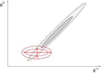
Figure 3: Illustrating the naive Gaussian sampler with fixed step sizes for two parameters. The (unknown) true likelihood surface is shown in black, the proposal distribution with arrows in red. This proposal distribution does not does not take into account the degeneracy among the parameters $\theta^{(1)}$ and $\theta^{(2)}$, leading to slow mixing.

Instead of using a naive Gaussian proposal distribution, we sample from a multivariate Gaussian distribution with covariance matrix estimated from the previous points in the chains. By taking into account the covariances among the parameters, we effectively approximate the likelihood contour in extent and orientation – the Gaussian samples are taken along the principal axis of the likelihood contour. Denoting $\theta_{i-1}-\theta_{i}=\bi{u}_{i}$ for notational convenience, the proposal distribution we use for the steps is

$$q(\theta_{i-1},\theta_{i})\sim N\exp\left[-\frac{1}{2}\bi{u}_{i}^{T}\bi{S}^{-1}\bi{u}_{i}\right],$$ (8)

where $N=\left(2\pi\right)^{-K/2}(\mbox{det}\,\bi{S})^{-1/2}$ and $\bi{S}$ is the covariance matrix

$$\bi{S}=\left(\begin{array}[]{cccc}\sigma_{1}^{2}&\rho_{12}&\dots&\rho_{1K}\\ \rho_{21}&\sigma_{2}^{2}&\dots&\rho_{2K}\\ \vdots&&\ddots&\vdots\\ \rho_{K1}&\dots&\rho_{K-1K}&\sigma_{K}^{2}\end{array}\right).$$ (9)

The sampling is most easily performed by diagonalizing the covariance matrix

$$\bi{T}^{T}\bi{S}\,\bi{T}=\bi{D}\Longleftrightarrow\bi{T}^{T}\bi{S}^{-1}\bi{T}=\bi{D}^{-1},$$ (10)

where $\bi{T}$ is an orthogonal matrix. Using this, equation (8) becomes

$$q(\theta_{i-1},\theta_{i})\sim N\exp\left[-\bi{u}_{i}^{T}\bi{T}\bi{T}^{T}\bi{S}^{-1}\,\bi{T}\bi{T}^{T}\bi{u}_{i}\right]$$ (11)

$$=N\exp\left[-\frac{1}{2}\bi{v}_{i}^{T}\bi{D}^{-1}\bi{v}_{i}\right],$$ (12)

where $\bi{v}_{i}\equiv\bi{T}^{T}\bi{u}_{i}$. Thus, the procedure for obtaining a sample $\bi{u}_{i}$ is as follows:

1. Find the eigenvalues $\tilde{\sigma}_{j}^{2}$ and eigenvectors of $\bi{S}$. Construct the transformation matrix $\bi{T}$ from the eigenvectors.

2. Draw Gaussian samples with variances $\tilde{\sigma}_{j}^{2}$, thereby obtaining the vector $\bi{v}_{i}$.

3. Then $\bi{u}_{i}=\bi{T}\bi{v}_{i}$ is the desired sample from the multivariate Gaussian with covariance matrix $\bi{S}$.

The convergence can be further improved by scaling the covariance matrix $\bi{S}$ with a variable factor $\alpha$. Using $\alpha$, we can cope better in situations where the projected likelihood takes on banana shapes such as in [24]. It also improves the convergence during the early stages when the low number of points available limits the estimate of the covariance matrix $\bi{S}$. We dynamically increase $\alpha$ if a chain takes steps too often, while we decrease $\alpha$ if the acceptance rate is too low. The positive effect of our scheme on the convergence is illustrated in figure 4.

One can show that modifying the proposal distribution based on previous chain data during the run may lead to a wrong stationary distribution $\pi^{\prime}(\theta|X)\$[29, 28]. Therefore, we only apply the dynamical strategy of finding an optimal step proposal during the early stages of the simulation. When the convergence is better than $R=1.2$ and the chain has calculated a certain number of points, we freeze in the step proposal distribution. All points in the chain before this freeze in should be discarded (see also A).

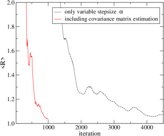
Figure 4: Convergence properties using different proposal distributions for a cosmological model with seven parameters. For illustration purposes we display the average $R$-statistic as a function of number of models computed. The univariate Gaussian proposal distribution using fixed variances but adaptive overall step size $\alpha$ (black dashed curve) shows convergence after about 2800 iterations. The multivariate Gaussian proposal distribution with covariance matrix estimated from the previous chain points and adaptive overall step size $\alpha$ as suggested in this paper (red solid curve) converges after 500 iterations.

3 The Software

The package is part of Cmbeasy and consists of two main components. The first one is a MCMC driver using LAM/MPI [32] for parallel execution of each chain. The second one is the AnalyzeThis class which is designed to evaluate the likelihood of a given model with respect to various data sets. These sets include the latest data of WMAP TT and TE [2, 3], ACBAR [4], CBI [5], VSA [6] , 2dFGRS [11, 12, 13], SDSS [14, 15], the SNe Ia compilations of Riess et al. [7], Tonry et al. [8] and Knop et. al. [9] as well as the IfA Deep Survey SNe Ia data [10]. Data files for all experiments are included for convenience. New data sets are added continuously to the code.

3.1 The MCMC Driver

The example MCMC driver consists of two routines: master() and slave(). Using LAM/MPI for parallel computing, one master and up to ten slaves may be started. The master() will determine the initial random starting position for each chain. In a never ending loop, it then sends the parameters to the slave()’s and collects the results when the computation is finished. Whenever a step has been successful, it stores the parameters and likelihoods of the last step together with the number of times the chain remained at the same point in parameter space in a new line of one file per chain. The format of these raw MCMC data files is defined in A. The master() monitors convergence and mixing and determines the next step for the slave(). Before freeze in, the covariance is estimated and the step proposal accordingly modified. After freeze in, the proposal distribution remains unchanged.

3.2 The AnalyzeThis Class

The AnalyzeThis class provides several routines concerning CMB, SNe Ia and Large Scale Structure measurements. It also contains routines for marginalizing and plotting the Monte Carlo data.

3.2.1 WMAP

The WMAP routines are (slightly modified) C++ ports of the likelihood code [25] available at the LAMBDA [33] web site. When the WMAP routines are called for the first time, the covariance matrices provided by WMAP will be converted to a binary format to speed up future use. A routine for WMAP normalization of the $C_{l}$ spectrum using the binned TT may be used instead of the old COBE normalization. (After the quick normalization, a best fit normalization may be called which uses the full likelihood routine provided by [25].)

3.2.2 ACBAR, CBI and VSA

We use the procedures for likelihood computation described by the ACBAR, CBI and VSA collaborations [4, 5, 6], using window functions and calibration uncertainty. One can de-select data bins from each of these datasets. It is, for instance, possible to calculate the likelihood for the low $l$ data only, thus speeding up the computation of a model, because the window functions of the high $l$ data require multipoles up to $l=4000$. One may also wish to exclude $l<800$ data if one is using the WMAP observations in order to keep the sets independent.

3.2.3 2dFGRS

For this Large Scale Structure dataset one compares the data with the theoretical power spectrum at $z=0.17$, the effective redshift of the survey, multiplied with the window function. We only include the region with $k/h<0.15\mbox{ Mpc}^{-1}$ since at smaller scales nonlinear effects need to be taken into account [11]. For these values, the bias is nearly constant [12, 13]. One may either specify the bias or marginalize over it.

3.2.4 SDSS

The theoretical power spectrum to be compared with the data should be evaluated at the effective redshift of this survey, at $z=0.1$. We use the data given in Table 3 of [14] and the appropriate window functions. One may select the maximum $k$-value to be included in the likelihood estimate, but including data beyond $k/h>0.15\mbox{ Mpc}^{-1}$ requires nonlinear corrections. Again, one can specify the bias or marginalize over it.

3.2.5 Supernovae Ia

We include four routines for calculating the likelihood with respect to SNe Ia data. Please note that the sets of Riess et al., Tonry et al. and Knop et al. are not independent.

Riess et. al.

One can use the full dataset, subset selection of the “gold” set as described in [7] is possible. Likelihood computation as given in this paper.

Tonry et. al.:

From the supernovae compilation of Tonry et al. [8] one can use the full data set of 230 Supernovae or, alternatively, one may use a restricted set of 172 supernovae, where supernovae with $z<0.01$ and with excess reddening have been omitted as suggested in [8]. In any case, we have taken the particular velocity uncertainty to be $v=500\mbox{ km/s}$ corresponding to $\Delta z=0.00167$ and computed the corresponding uncertainty in the luminosity distance to obtain the likelihood:

$$\chi^{2}=\sum_{i=1}^{N}\frac{(\log d_{l}^{exp}-\log d_{l}^{th})^{2}}{\sigma_{tot}^{2}},$$ (13)

$$\mbox{with }\sigma_{tot}^{2}=\sigma_{exp}^{2}+\left(\frac{d\log d_{l}^{th}}{dz}\right)^{2}\Delta z^{2}.$$ (14)

Here, $d_{l}^{exp}$ and $d_{l}^{th}$ is the experimental and theoretical luminosity distance, respectively.

Knop et. al.:

The 54 SNe Ia presented in Tables 3-5 [9] have been included in the code. We use the data with strech and extinction correction applied, subsample selection as discussed in [9] is also possible.

IfADS survey:

One may choose to include all 23 SNe Ia given in [10], or one may exclude the supernovae with excess reddening and those not unambigously identified as SNe Ia as described in [10].

3.3 The Graphical User Interface

The gui may be used to process the raw output files of the MCMC chains. After starting cmbeasy, the first step is to “distill” the chain data files. By distilling we mean the merging of the raw chain output files into one file. In addition, distilling removes all burn-in data. To get started immediately, we include raw data from an example MCMC run in the resources directory of cmbeasy. The four chains are called montecarlo_chain$\alpha$.dat. They are runs for a $\Lambda$CDM model and need to be distilled first. Two and one dimensional marginalized likelihoods may then be plotted and printed from within the gui (see figure 1). Please see the “howto-montecarlo” document shipped with cmbeasy for an introduction.

4 Cosmological constraints from the data sets

Having described the method and software, we can now proceed to investigate the impact of the different data sets on the distribution of parameters for a given cosmological model. For illustrative purposes we limit ourselves to a flat $\Lambda$CDM cosmology with five parameters. We take the reduced baryon and matter densities $\Omega_{b}h^{2}$ and $\Omega_{m}h^{2}$, the Hubble parameter $h=H_{0}/(100\mbox{km s}^{-1}\mbox{Mpc}^{-1})$, the optical depth to the last scattering surface $\tau$ and the spectral index of the initial power spectrum $n_{s}$ as parameters. We neglect any tensor contributions and we marginalize over the amplitude of the initial power spectrum. Thus, the amplitude is treated as a “nuisance” parameter that is integrated out.

In table 1 we display the cosmological parameters and the flat priors used.

Table 1: Flat priors on the parameters used in our MCMC simulations

• Parameter	Min	Max
  $\Omega_{b}h^{2}$	0.016	0.03
  $\Omega_{m}h^{2}$	0.05	0.3
  $h$	0.60	0.85
  $\tau$	0	0.9
  $n_{s}$	0.8	1.2

The limits of the parameter ranges are chosen in accordance with previous results [1, 14].

First, we will investigate constraints from CMB-only data, subsequently adding Supernovae Ia and large scale structure data sets. For a detailed description of how we implemented the datasets we refer the reader to section 3.2 of this paper. We have performed three MCMC simulations with CMB only, CMB+ SNe Ia and CMB + SNe Ia + LSS data sets. Convergence was reached in each run after about $\sim 2000$ iterations, each simulation was run until 55 000 models had been computed.

For the CMB-only run we use the measurements of WMAP (TT and TE spectra), CBI, VSA and ACBAR up to $l=2000$, removing data points from CBI, VSA and ACBAR where we have WMAP measurements with comparable error bars to keep the data sets independent. The entire set we used is displayed in figure 5.

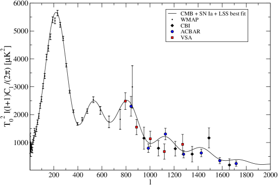
Figure 5: CMB data set for constraining cosmological parameters.

For CMB + SNe Ia we add the data set of Riess et al. [7] (“gold sample”), and finally for CMB + SNe Ia + LSS we add the large scale structure measurements of the SDSS collaboration using all points with $k/h<0.15\;\mbox{Mpc}^{-1}$ where the perturbations are still linear [15]. The results are presented in table 2, marginalized likelihoods for the parameters are displayed in table 3 and figure 6.

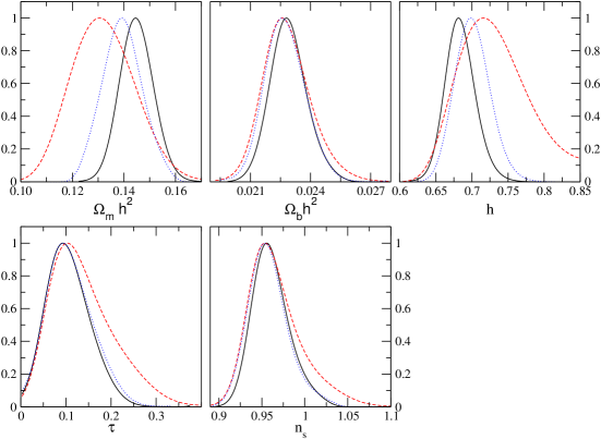
Figure 6: One dimensional marginalized distributions for the parameters. Constraints from CMB only (red, dashed), CMB + SNe Ia (blue, dotted) and CMB + SNe Ia + LSS (black, solid). The histograms extracted from the chains were fitted using a function $f(x)=\exp(p(x))$ with $p(x)$ a sixth-order polynomial [14].

Table 2: Constraints on the parameters from a combination of data sets. These confidence intervals were generated from the one-dimensional marginalized distributions (errors are given at 68.3 % confidence level).

• Parameter	CMB only	CMB + SNe Ia	CMB+ SNe Ia + LSS
  $\Omega_{b}h^{2}$	$0.02261^{+0.0012}_{-0.0011}$	$0.02257^{+0.0011}_{-0.0009}$	$0.02278^{+0.0009}_{-0.0009}$
  $\Omega_{m}h^{2}$	$0.1306^{+0.013}_{-0.012}$	$0.1393^{+0.0076}_{-0.008}$	$0.144^{+0.0063}_{-0.0066}$
  $h$	$0.716^{+0.053}_{-0.041}$	$0.699^{+0.024}_{-0.024}$	$0.682^{+0.021}_{-0.021}$
  $\tau$	$0.1019^{+0.081}_{-0.52}$	$0.0941^{+0.058}_{-0.043}$	$0.0938^{+0.051}_{-0.0043}$
  $n_{s}$	$0.954^{+0.032}_{-0.024}$	$0.953^{+0.024}_{-0.021}$	$0.956^{+0.023}_{-0.019}$

Table 3: Two-dimensional marginalized likelihoods for the cosmological parameters using CMB + SNe Ia + LSS data. The contours are one, two and three sigma confidence regions, respectively.

We will now discuss the impact of the different sets on the parameters. Consider figure 6. The CMB-only data set does not well constrain $\Omega_{m}h^{2}$. Adding supernovae improves the bounds on the total matter content considerably, because the lumiosity distance depends sensitively on $\Omega_{m}$. Adding large scale structure data breaks the degeneracy between matter contribution and initial power spectrum amplitude, hence we obtain still tighter bounds. Note that the distribution of $\Omega_{m}h^{2}$ obtained from CMB-only and CMB + SNe Ia + LSS data sets differ somewhat. This has already been noted in [14]. Even from CMB measurements alone we can infer the presence of dark matter at high significance. In contrast, the baryon contribution $\Omega_{b}h^{2}$ is already well constrained by the CMB alone, adding SNe Ia and LSS data only improves the bounds slightly. The CMB is most sensitive to this parameter since what one observes are essentially oscillations in a photon-baryon plasma, the density of baryons is a critical parameter for the shape of the CMB spectrum. SNe Ia and LSS measurements are more or less insensitive to this parameter, though hints at oscillations in the power spectrum have been detected [11].

The Hubble parameter $h$, is only slightly constrained by CMB measurements alone. Adding SNe Ia data considerably improves the bounds, adding large scale structure data does not improve the bounds very much. The bounds obtained for the Hubble parameter for the full data set are consistent with the HST key project value $h=0.72\pm 0.08$ [34] derived from measuring the local Hubble flow. Even though the optical depth does not directly influence SNe Ia predictions, adding SNe Ia data tightens the bound on the optical depth $\tau$ as seen in figure 6. The mechanism is somewhat indirect: SNe Ia data tightens the bound on $\Omega_{m}$ and thus limits the range of allowed values for $\tau$, $h$ and $n_{s}$ from CMB measurements. As we marginalize over the bias of the SDSS data, large scale structure does not add further to the bounds on $\tau$.

5 Conclusions

We have introduced the AnalyzeThis package, which can be used to constrain cosmological models using observational data sets. The AnalyzeThis class provides many functions to compute the likelihood of a model with respect to measurements of the CMB, SNe Ia and Large Scale Structure.

In order to constrain models of the Universe with a substantial number of parameters, we include a Markov Chain Monte Carlo driver. As the MCMC step strategy determines the convergence speed of the chains, we implemented a multivariate Gaussian sampler with an additional dynamical scaling. We stop the adaptive improvement of the step proposal density as soon as a good level of convergence is reached and discard all data calculated before. Using this approach, we combine the advantage of a single-run automatic optimization of the step strategy with the demand of a static step proposal density.

The output of the Monte Carlo chains is in a human readable format and may be processed by any software, even during the run. For convenience however, one may use Cmbeasy’s gui to marginalize, plot and print two and one dimensional likelihood surfaces.

Finally, we discussed the impact of the different data sets on the parameters for the case of a $\Lambda$CDM cosmology with five parameters.

Appendix A Files and Formats

A.1 MCMC chain output data

The parameters and likelihoods of each model are stored in files with the naming convention “montecarlo_chain$\bi{\alpha}$.dat”, where “$\bi{\alpha}$” is an integer. Each file corresponds to a slave() process (and hence to an independent chain). Each line in such a file represents a new point in parameter space. The format of one such line is:

$$p_{0}\ |\ p_{1}\ |\dots|p_{n}\ |\ L\ |\ l_{0}\ |\ \dots|\ l_{m}\ |\ a_{1}\ |\ \dots|\ a_{k}\ |\ M,$$

where $p_{i}$ are the parameters of the model, $L$ is the overall likelihood, the $l_{i}$ are likelihoods of different experiments, $a_{i}$ are auxiliary fields (to store $\sigma_{8}$, for instance). Finally, $M$ determines the weight of this parameter set, i.e. the “time” spend before leaving this point in parameter space. When the step sizes and the covariance estimates are frozen in, one line in each file gets a zero $M$. All data before this line should be regarded as “burn-in”. The graphical user interface (using the distillChains() routine of AnalyzeThis) will automatically discard all models before freeze-in.

A.2 Monitoring Progress and Covariance

The master() routine outputs the convergence and some more information into a file called “progress.txt”. Until the step proposal distribution is frozen in, the covariance matrix is in addition output to “covMatrix.txt”. Messages of any errors occuring in slave() will be appended to the file “errorlog.txt”.

References

- [1] C. L. Bennett et al., “First Year Wilkinson Microwave Anisotropy Probe (WMAP) Observations: Preliminary Maps and Basic Results,” Astrophys. J. Suppl. 148 (2003) 1 [arXiv:astro-ph/0302207]
- [2] G. Hinshaw et al., “First Year Wilkinson Microwave Anisotropy Probe (WMAP) Observations: Angular Power Spectrum,” Astrophys. J. Suppl. 148 (2003) 135 [arXiv:astro-ph/0302217]
- [3] A. Kogut et al., “Wilkinson Microwave Anisotropy Probe (WMAP) First Year Observations: TE Polarization,” Astrophys. J. Suppl. 148 (2003) 161 [arXiv:astro-ph/0302213]
- [4] C. l. Kuo et al. [ACBAR collaboration], “High Resolution Observations of the CMB Power Spectrum with ACBAR,” Astrophys. J. 600 (2004) 32 [arXiv:astro-ph/0212289]
- [5] A. C. S. Readhead et al., “Extended Mosaic Observations with the Cosmic Background Imager,” arXiv:astro-ph/0402359
- [6] C. Dickinson et al., “High sensitivity measurements of the CMB power spectrum with the extended Very Small Array,” arXiv:astro-ph/0402498
- [7] A. G. Riess et al., “Type Ia Supernova Discoveries at z¿1 From the Hubble Space Telescope: Evidence for Past Deceleration and Constraints on Dark Energy Evolution,” arXiv:astro-ph/0402512
- [8] J. L. Tonry et al., “Cosmological Results from High-z Supernovae,” Astrophys. J. 594 (2003) 1 [arXiv:astro-ph/0305008]
- [9] R. A. Knop et al., “New Constraints on , , and w from an Independent Set of Eleven High-Redshift Supernovae Observed with HST,” arXiv:astro-ph/0309368
- [10] B. J. Barris et al., “23 High Redshift Supernovae from the IfA Deep Survey: Doubling the SN Sample at z¿0.7,” Astrophys. J. 602 (2004) 571 [arXiv:astro-ph/0310843]
- [11] W. J. Percival et al., “The 2dF Galaxy Redshift Survey: The power spectrum and the matter content of the universe,” Mon. Not. Roy. Astron. Soc. 327, 1297 (2001) arXiv:astro-ph/0105252
- [12] L. Verde et al., “The 2dF Galaxy Redshift Survey: The bias of galaxies and the density of the Universe,” Mon. Not. Roy. Astron. Soc. 335, 432 (2002). [arXiv:astro-ph/0112161]
- [13] J. A. Peacock et al., “A measurement of the cosmological mass density from clustering in the 2dF Galaxy Redshift Survey,” Nature 410 (2001) 169 [arXiv:astro-ph/0103143]
- [14] M. Tegmark et al. [SDSS Collaboration], “Cosmological parameters from SDSS and WMAP,” arXiv:astro-ph/0310723
- [15] M. Tegmark et al. [SDSS Collaboration], “The 3D power spectrum of galaxies from the SDSS,” arXiv:astro-ph/0310725
- [16] U. Seljak and M. Zaldarriaga, “A Line of Sight Approach to Cosmic Microwave Background Anisotropies,” Astrophys. J. 469 (1996) 437 [arXiv:astro-ph/9603033]
- [17] A. Lewis, A. Challinor and A. Lasenby, “Efficient Computation of CMB anisotropies in closed FRW models,” Astrophys. J. 538 (2000) 473 [arXiv:astro-ph/9911177]
- [18] M. Doran, “CMBEASY:: an Object Oriented Code for the Cosmic Microwave Background,” arXiv:astro-ph/0302138
- [19] N. Christensen and R. Meyer, “Bayesian Methods for Cosmological Parameter Estimation from Cosmic Microwave Background Measurements,” arXiv:astro-ph/0006401
- [20] N. Christensen, R. Meyer, L. Knox and B. Luey, “II: Bayesian Methods for Cosmological Parameter Estimation from Cosmic Microwave Background Measurements,” Class. Quant. Grav. 18 (2001) 2677 [arXiv:astro-ph/0103134]
- [21] A. Lewis and S. Bridle, “Cosmological parameters from CMB and other data: a Monte-Carlo approach,” Phys. Rev. D 66 (2002) 103511 [arXiv:astro-ph/0205436]
- [22] L. Knox, N. Christensen and C. Skordis, “The Age of the Universe and the Cosmological Constant Determined from Cosmic Microwave Background Anisotropy Measurements,” Astrophys. J. 563 (2001) L95 [arXiv:astro-ph/0109232]
- [23] R. R. Caldwell and M. Doran, “Cosmic microwave background and supernova constraints on quintessence: Concordance regions and target models,” arXiv:astro-ph/0305334
- [24] A. Kosowsky, M. Milosavljevic and R. Jimenez, “Efficient Cosmological Parameter Estimation from Microwave Background Anisotropies,” Phys. Rev. D 66 (2002) 063007 [arXiv:astro-ph/0206014]
- [25] L. Verde et al., “First Year Wilkinson Microwave Anisotropy Probe (WMAP) Observations: Parameter Estimation Methodology,” Astrophys. J. Suppl. 148 (2003) 195 [arXiv:astro-ph/0302218]
- [26] A. Slosar and M. Hobson, “An improved Markov-chain Monte Carlo sampler for the estimation of cosmological parameters from CMB data,” arXiv:astro-ph/0307219
- [27] W. R. Gilks, S. Richardson, and D. J. Spiegelhalter, “Markov Chain Monte Carlo In Practice”,(Chapman and Hall, London, 1996).
- [28] D. Gamerman, “Markov Chain Monte Carlo”, (Chapman and Hall, London, 1997).
- [29] R. M. Neal (1993), ftp://ftp.cs.utoronto.ca/pub/radford/review.ps.Z.
- [30] N. Metropolis, A. W. Rosenbluth, M. N. Rosenbluth, A. H. Teller and E. Teller, “Equation Of State Calculations By Fast Computing Machines,” J. Chem. Phys. 21 (1953) 1087
- [31] A. Gelman, and D. B. Rubin, “Inference from iterative simulation using multiple sequences,” Statist. Sci. 7 (1992) 457-511
- [32] http://www.lam-mpi.org/
- [33] http://lambda.gsfc.nasa.gov
- [34] W. L. Freedman et al., “Final Results from the Hubble Space Telescope Key Project to Measure the Hubble Constant,” Astrophys. J. 553 (2001) 47 [arXiv:astro-ph/0012376]