A spectral and spatial analysis of $\eta$ Carinae’s diffuse X-ray emission using CHANDRA

The luminous unstable star (star system) $\eta$ Carinae is surrounded by an optically bright bipolar nebula, the Homunculus and a fainter but much larger nebula, the so-called outer ejecta. As images from the EINSTEIN and ROSAT satellites have shown, the outer ejecta is also visible in soft X-rays, while the central source is present in the harder X-ray bands. With our CHANDRA observations we show that the morphology and properties of the X-ray nebula are the result of shocks from fast clumps in the outer ejecta moving into a pre-existing denser circumstellar medium. An additional contribution to the soft X-ray flux results from mutual interactions of clumps within the ejecta. Spectra extracted from the CHANDRA data yield gas temperatures $kT$ of $0.6-0.76$ keV. The implied pre-shock velocities of 670-760 km s^-1 are within the scatter of the velocities we measure for the majority of the clumps in the corresponding regions. Significant nitrogen enhancements over solar abundances are needed for acceptable fits in all parts of the outer ejecta, consistent with CNO processed material and non-uniform enhancement. The presence of a diffuse spot of hard X-ray emission at the S condensation shows some contribution of the highest velocity clumps and further underlines the multicomponent, non-equilibrium nature of the X-ray nebula. The detection of an X-ray “bridge” between the northern and southern part of the X-ray nebula and an X-ray shadow at the position of the NN bow can be attributed to a large expanding disk, which would appear as an extension of the equatorial disk. No soft emission is seen from the Homunculus, or from the NN bow or the “strings”.

1 Introduction

1.1 The object: $\eta$ Carinae

With luminosity $L\sim 10^{6.7}\,L_{\sun}$, $\eta$ Car marks the upper boundary of the empirical Hertsprung-Russell diagram (HRD). It is one of the most massive stars known ($M>120\,M_{\sun}$), somewhat evolved, and unstable; see e.g. Humphreys & Davidson (1994), Davidson & Humphreys (1997) and Hillier et al. (2001).

In the optical, $\eta$ Carinae is known to be an irregularly variable source.  The historical lightcurve covers several centuries and shows the star’s most sudden change around 1843 when it brightened to $-$1^m (Herschel 1847; Innes 1903; Viotti 1995; Humphreys et al. 1999) and drastically decreased its brightness by more than 7^m during the following 20 years, an event known as the “Great Eruption”.

$\eta$ Carinae is an evolved massive star, now classified a Luminous Blue Variable (LBV). LBVs are very massive stars in a transitional phase between the main-sequence and the Wolf-Rayet state. Only stars above $\sim$ 50 M_☉ enter this unstable phase, which occurs at an age of roughly 3 10⁶ years (e.g. Langer et al. 1994). After the main-sequence phase such stars first evolve towards the red, cooler regime in the HRD, but as they enter the LBV phase they reverse their evolution before becoming red supergiants. The temperature-dependent luminosity boundary in the HRD near which LBVs are situated is known as the Humphreys-Davidson Limit (HD-Limit; Humphreys & Davidson 1979, 1994).

A periodicity first found in high excitation lines (Damineli 1996, Damineli et al. 1997) and in $2-10$ keV X-ray emission (Corcoran et al. 1995, 2001a; Ishibashi et al. 1999) from the star raised the possibility that $\eta$ Carinae is a binary system. In such a system a wind eclipse of a shock produced by the the colliding winds from two hot stars would be responsible for the observed X-ray variability. In this scenario, $\eta$ Carinae, the more massive component, has a mass in excess of 60 M_☉ while the companion would have a mass of about $30-60$ M_☉ (Damineli et al. 1997, Corcoran et al. 2001a). For further information concerning the high-energy X-ray emission in connection with the central source we refer the reader to, for e.g., Ishibashi et al. (1999), Corcoran et al. (2001a,b), Pittard & Corcoran (2002) and references therein.

1.2 The Homunculus nebula: optical and X-ray emission

One of the main characteristics of the LBV phase is the star’s optical variability, which occurs on different timescales and amplitudes: from a few tenths of a magnitude within several months, to $1-2$ magnitude variations on timescales of decades, to variations of several magnitudes as seen in the giant eruptions which occur probably once or twice during the LBV phase. Whether all LBVs undergo giant eruptions is not clear. Therefore LBVs are sometimes divided into the “S Dor” variables and the “eruptive” variables depending on whether or not an eruption has taken place (Humphreys 1999). $\eta$ Carinae is the canonical eruptive-type LBV. Together with the high increase in mass loss which occurs during the LBV phase (several $10^{-4}$ M${}_{\sun}\,{\rm yr}^{-1}$ at least) these eruptions – in which the stars peel of large parts of their outer envelopes – are responsible for the formation of LBV nebulae (Nota et al. 1995; Weis 2001a).

The bright ejecta-nebula around $\eta$ Carinae was first clearly identified in the 1940s (Gaviola 1946, 1950; Thackeray 1949, 1950) when it was about 30% smaller than today. Gaviola called it the Homunculus because it resembled a little man in his photographs. At high spatial resolution, it has become one of the most dramatic examples of bipolar morphology, having two roughly symmetric polar lobes and an equatorial disk of material (Duschl et al. 1995) which is sometimes called the skirt (e.g. Morse et al. 1998). Its polar diameter is currently about 17″ or 0.2 pc. Fainter condensations outside the Homunculus were also detected more than 50 years ago (Thackeray 1949; Walborn 1976), and manifest a much larger outer nebula, seen in deep HST images (e.g. Weis 2001a) and images in the soft X-ray energy band. This outer ejecta, which consists of a large collection of “bullets”, “knots” and “filaments”, has a diameter of about 60″ or 0.67 pc. Figure 1 displays an HST image taken in July 1997 in the F658N filter, which shows a mixture of H_α and [N ii] emission. Here the intensity levels are chosen to show the faint outer material, and we have indicated the location and size of the bipolar Homunculus by contours.

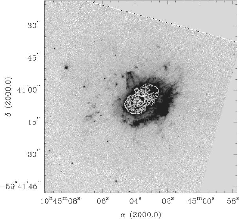
Figure 1: An HST F658N image which shows the optical emission from $\eta$ Carinae’s Homunculus and the outer ejecta. The contrast has been optimized to show the fainter outer emission. The bright central region including the bipolar Homunculus is displayed using contours.

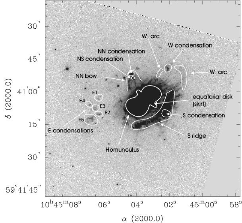
Figure 2: Previously identified features in the Homunculus and the outer ejecta are marked. Part of the nomenclature is according to Walborn et al. (1978)

Both parts of the nebula – the Homunculus and the outer ejecta – are expanding. The expansion velocity of the Homunculus is about 650 km s^-1 (Thackeray 1961; Davidson & Humphreys 1997) while in the outer ejecta observed velocities average at roughly 600 km s^-1 – slow enough to suggest either an earlier ejection date or else deceleration – and reach maximum expansion velocities up to 2000 km s^-1 or more (Weis 2001a,b; Weis et al. 2001). We will show in an upcoming paper that it is indeed possible that the outer ejecta was created 1843 and has been slowed down (Weis & Duschl, in prep.).

The outer ejecta produces soft X-rays. The EINSTEIN satellite separated the nebular from the stellar X-ray emission (Chlebowski et al. 1984), while images with spatial resolution $\sim$ 5″ were obtained later with the High Resolution Imager (HRI) aboard the Röntgensatellite, ROSAT. Weis et al. (2001) presented a detailed analysis of the ROSAT data and a comparison with optical images and kinematic data. The X-ray nebula is hook-shaped, with X-ray bright knots near the locations of the prominent S ridge and W arc (features named by Walborn 1978, see also Figs. 2, 5). Considering also the kinematic data, it thus became clear that shocks associated with fast-moving visible knots produce much of the observed diffuse soft X-ray flux. Since the outer knots and filaments have characteristic sizes ranging from a small fraction of an arcsecond to several arcseconds, the shock structures were not well resolved in the ROSAT images. Seward et al. (2001) reported the first CHANDRA X-ray images in the $0.2-10$ keV band using the Advanced CCD Imaging Spectroscopy (ACIS) imaging array with resolution $\approx 1\arcsec$ and compared them to HST images. However, the energy resolution of this early CHANDRA observation was seriously degraded by radiation damage which severely hampered the search for spectral variations in the nebulosity. Here we describe a spatially resolved analysis of the X-ray nebulosity around $\eta$ Car, based on a the zeroth-order image from a deep observation obtained using the CHANDRA High Energy Transmission Grating and the ACIS spectroscopic array.

1.3 Aim and advances of the new CHANDRA observations

We used a dataset which was obtained by the CHANDRA X-ray Observatory primarily to obtaine a grating spectrum of the central source. CHANDRA images have about 10 times better spatial resolution than ROSAT HRI, allowing us to better define the X-ray source regions and possible coincidences with optical counterparts. Even though the X-ray resolution is still a factor of 5 worse than the best optical images, we can now constrain the identifications fairly well. In addition to morphological comparisons of X-ray, optical and kinematic data (see also Weis et al. 2001), we can also explore the X-ray spectral properties of selected regions in the ejecta.

Our new data and results are presented in the following way. Sect. 2 describes the new X-ray observations and their reduction; Sect. 3 briefly summarizes earlier work and data sets which are necessary and useful for this paper. In Section 4 we discuss new results from the CHANDRA data. Section 5 contains a comparison between the X-ray data and the kinematics of the optical gas, while in Sect. 6 we present a discussion of our results, and we summarize the main results in Sect. 7.

2 CHANDRA Observations

$\eta$ Carinae was observed on 2000 November 19 with CHANDRA’s Advanced CCD Imaging Spectrometer (ACIS) and High Energy Transmission Grating (HETG). We used the 0th order image situated at the aimpoint on the S3 chip, obtaining spectral information from numbers of electrons in photon-detection events rather than from the dispersed spectrum. The spatial resolution was about 1″ and the exposure time was 91 ksec. The data were screened for bad events, rejecting events graded 1, 5 and 7. We produced three separate images representing photon energy ranges 0.2–0.6, 0.6–1.2, and 1.2–11 keV by using the FSELECT and XSELECT tasks in the HEASOFT software package. Figure 3 shows the CHANDRA X-ray image in the $0.2-11$ keV band while Figure 4 shows the images in the 3 energy bands separately.

Spectra of selected areas were extracted and analyzed using the HEASOFT tasks XSELECT and XSPEC. The spectral resolution is roughly 0.13 keV in the $0.2-1.5$ keV energy range. First we extracted a spectrum of the entire X-ray nebula, excluding the central object. Then we extracted spectra from the five relatively bright regions shown in Figure 5, along with the spectrum of the central object (which suffers from photon event pileup) for comparison. Each of the five selected areas represents either an identifiable, coherent large-scale structure or an area of special interest identified by earlier work, e.g., “knot 2” as discussed by Weis et al. (2001). These selections were also constrained by the need for good photon statistics. Their names in Fig. 5 correspond to visual-wavelength features identified by Walborn (1978; see Fig. 2). Each spectrum was corrected for background, using background samples close enough to $\eta$ Car so that the intervening absorbing column density was approximately constant. Since the diffuse X-ray emission in the Carina H ii region varies spatially (e.g. Seward & Chlebowski 1982), we compared spectra from a variety of nearby regions when constructing background spectra.

3 Supporting work and datasets

3.1 HST images

We compared the X-ray emission to optical images obtained with the Hubble Space Telescope (HST) and the Wide Field Camera (WFPC). Suitable data were retrieved from the STScI archive. In order to map the faint outer knots which are the main contributors to the X-ray shocks (Weis et al. 2001), we selected four images that used WFPC2 filter F658N (see below), exposed for 2 $\times$ 200 s and 2 $\times$ 4 s. The short exposures were used to correct CCD bleeding in the longer exposures. Data from all four WFPC2 quadrants were combined as a mosaic, with spatial resolution about 0$\aas@@fstack{\prime\prime}$0996 per pixel and a field large enough to include a few stellar X-ray sources, which served as astrometric reference points for aligning the CHANDRA and HST images. Figure 1 shows the resulting F658N image. Here the display intensity is optimized to show the filamentary outer ejecta; the bipolar Homunculus is saturated in this rendition but we have marked it with intensity contours.

Finally, a note concerning F658N, which is usually considered to be either a [N ii] $\lambda$6586 emission line filter or else a redshifted H_α $\lambda$6565 filter. Since the outer ejecta studied here have a wide range of velocities, both emission lines contribute to Fig. 1 with spatially-dependent efficiencies. [N ii] is generally brighter in this gas (Davidson et al. 1986), but H_α dominates the image at locations where the knots are sufficiently redshifted, while neither line shows the blueshifted material well with this filter. We chose F658N rather than F656N, because images taken with the latter have much worse CCD bleeding from the central star’s intense H_α emission.

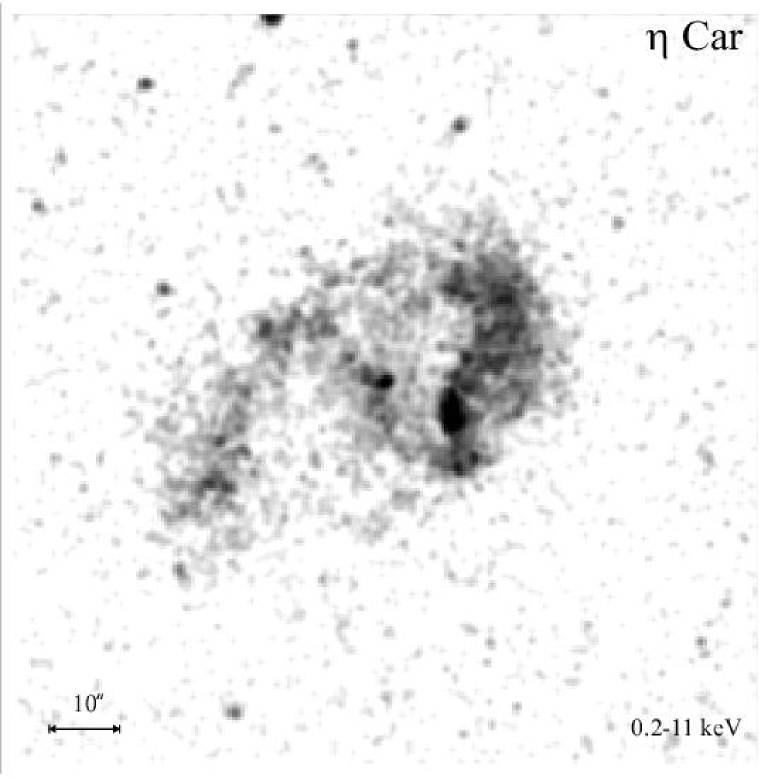
Figure 3: This figure shows a grayscale image of the X-ray emission of $\eta$ Carinae’s outer ejecta and the star, in the energy range between 0.2-11 keV. The intensity levels are optimized to emphasize the softer emission (roughly between 0.5-1.2 keV) from the ejecta. The bright, hard emission of the central object is therefore less pronounced.

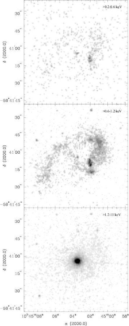
Figure 4: ACIS-S3 CHANDRA images of $\eta$ Carinae in different energy bands. Upper panel: energy range $0.2-0.6$ keV, dominated by the nitrogen K emission line (see text for details). Middle panel: energy range $0.6-1.2$ keV. Lower panel: emission at energies $1.2-11$ keV, where the star dominates the emission.

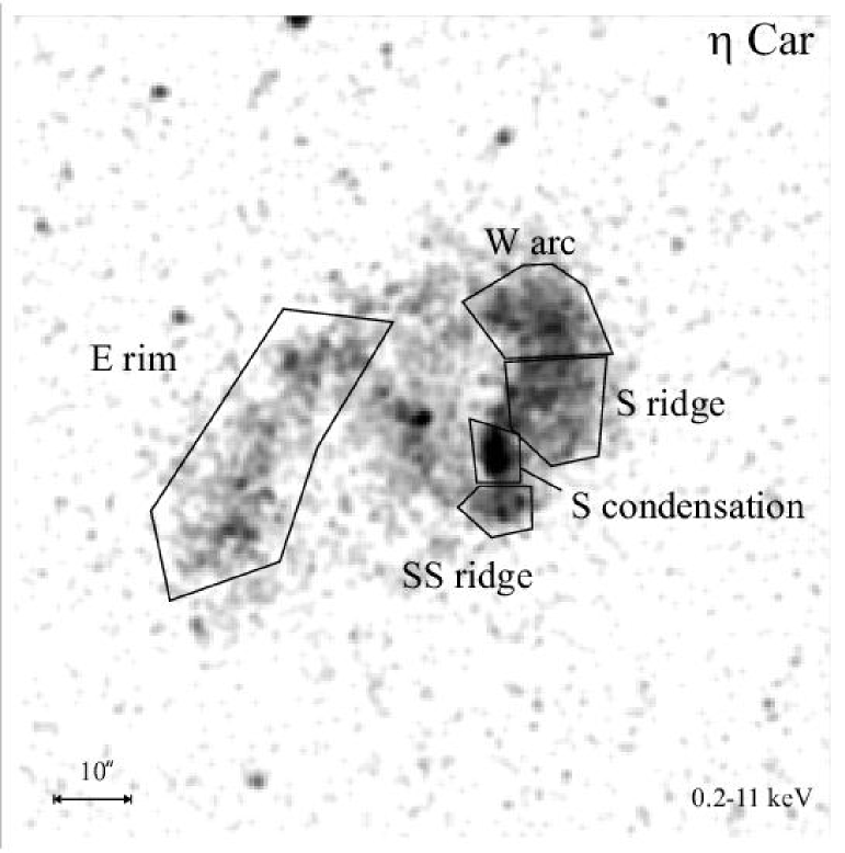
Figure 5: CHANDRA full band image in which the X-ray emitting regions in the outer ejecta are subdivided and named to follow the nomenclature used to describe the optical features (Walborn et al.  1978, see also Fig. 2).

3.2 Echelle Spectra - Kinematics

We used optical spectra to determine local expansion velocities, for comparison with both the optical image and the X-ray data. This analysis was similar to that reported by Weis et al. (2001); in fact we used the same kinematic data set. Since Weis et al. described these spectra in detail, here we merely summarize the essential facts. Data were obtained with the Echelle spectrograph of the 4 m telescope at Cerro Tololo Interamerican Observatory. The outer ejecta were mapped with 32 slit positions; the slit was oriented at position angle 132°  i.e., parallel to the major axis of the Homunculus, and successive slit centerlines were 1$\aas@@fstack{\prime\prime}$4 apart. Severe stray light within the instrument spoiled six of the central spectra. The FWHM spectral resolution was 14 km s^-1 across a spectral range of 75 Å centered on H_α, while spatial resolution, limited by seeing, varied between 1$\aas@@fstack{\prime\prime}$4 and 2″ during the observations.

4 CHANDRA Results

4.1 CHANDRA images

4.1.1 The morphology of the X-ray emission

We extracted images in three energy bands from the ACIS S3 data. The total-band zeroth-order image ($0.2-11$ keV) was smoothed (using a gaussian smoothing with $\sigma=0.8$) and is displayed in greyscale in Fig. 3. Images in individual energy bands are shown in Fig. 4. The softest energy band spans $0.2-0.6$ keV. As will be seen later from the spectra (see section 4.2), the predominant emission in this band is from the nitrogen K lines (see next section). The intermediate energy band ($0.6-1.2$ keV, the middle panel in Fig. 4) will be of principal interest in the upcoming discussion since it contains most of the X-ray emission contributed by the outer ejecta. The central source is only barely visible in this energy range. At higher energies ($1.2-11$ keV, bottom panel, Fig. 4), the emission from the central source dominates. Since our main interest here is the diffuse soft X-ray emission we do not discuss in detail the hard-band emission from the central object (see Corcoran et al. 2001b and Pittard & Corcoran 2002 for a more detailed discussion of the X-ray spectral energy distribution of the central source). We will however use the images and spectra of the hard X-ray emission – and therefore the central object – to compare with the properties of the softer emission of the outer nebula. Also, since the morphology of the X-ray nebula in the nitrogen K line and at intermediate energies are similar, but the nitrogen K line image has poor signal-to-noise, we will concentrate our following discussion on the intermediate-band (0.6 to 1.2 keV) images.

The X-ray nebula in the energy range $>0.6-1.2$ keV (Fig. 4 middle panel) is roughly hook shaped (sometimes referred to as the “shell”), as previously seen in the ROSAT images (Weis et al. 2001). Analysis of an early CHANDRA image implied that the X-ray nebula is a ring rather than a limb-brightened elllipsoidal shell (Seward et al. 2001) due to the lack of emission in the center. The limited spatial resolution of the ROSAT images led Weis et al. (2001) to attribute the majority of the emission to two individual X-ray emission regions which they called “knot 1” and “knot 2”. The higher spatial resolution of CHANDRA separates these knots into several individual components. The region originally called knot 1 contains at least two bright components. The center of knot 1 is now identified with the S condensation (see nomenclature in Fig. 5), while knot 1 included (at least partially) an area we now call the “SS ridge” (since it lies just south of the optical feature known as the S ridge). Combining the S condensation and SS ridge yields a region of emission which matches well the triangular shaped knot 1 of Weis et al. 2001. We identify knot 2 with the X-ray bright regions near the W arc in Fig.  5. We identify the X-ray bright region between the W arc and the S condensation as the S ridge since it coincides with the northeast extension of the optical S ridge. Finally, as seen in Fig.  5, we identify a large section of X-ray emission in the east as the “E rim”. The southwestern part of the E rim includes optically identified features called the E condensations (see Fig. 2), but the X-ray emission stretches further out than these optical emission features.

The CHANDRA intermediate-band image clearly shows a new feature, a band of diffuse emission that crosses the Homunculus connecting the SS ridge to the E rim just slightly south of the central point source (see Sect. 6.4). We refer to this feature as the “bridge”. From ROSAT HRI images, Weis et al. (2001) speculated about a possible elongation of the central source with a position angle of 30°. This is roughly the same as the orientation of the bridge (keeping in mind the lower resolution of the ROSAT images). Therefore we conclude that the elongated X-ray emission at the position of the central source seen by ROSAT actually was a detection of the “bridge”. The CHANDRA images show that the central X-ray source, however, is consistent with point-like emission. The intermediate-band CHANDRA image (Fig. 4, middle panel) shows a deficit of X-ray emission in the west just to the north of the “bridge”, between (clockwise) the end of the E rim and the beginning of the W arc.

The $1.2-11$ keV image shows nearly exclusively the bright hard central source. As previously noted (Seward et al. 2001) CHANDRA images (Fig. 4) seem to indicate that the central point source is surrounded by a halo of relatively hard emission reaching out into the W arc, S condensation and S ridge regions which is partly due to the wings of the point spread function (PSF), and partly due to some real hard diffuse emission. Although the region near $\eta$ Car is badly contaminated by the wings of the point spread function of the bright central source, Fig. 6 suggests that some real hard X-ray emission may exist in the Homunculus, similar to the “halo” noted by Seward et al. (2001), and possibly in the outer nebula as well (see Sect. 6.5). In order to investigate whether any real hard emission originates in the region around $\eta$ Carinae, we attempted to model the radial brightness distribution of the central source. We used the CHANDRA Interactive Analysis of Observations (CIAO) software package to generate a model PSF based on the CHANDRA PSF library and the procedure outlined in the CIAO science threads. We chose a central energy of 4.5 keV to generate the PSF, based on the spectrum of the central source (see Fig. 7), and we used tasks in IRAF/STSDAS for the comparison of the PSF to our data. We smoothed the model PSF image with the same $\sigma=0.8$ Gaussian as the observed hard-band image. Additionally we corrected the centering of the model PSF to agree with the peak position of the hard source by fitting Gaussian and Moffat functions. The centering of the two images agreed after this process to better than 0.2 pixel. We then attempted to scale the PSF to the peak flux of the central source. This scaling is inexact, because the central source suffers from severe photon pile-up which causes the intensity of the central source to be underestimated by a large amount. We experimented with various scalings of the model X-ray PSF to the observed PSF to find the maximum contribution from the wings of the point source. We found that even if we adopt a scaling factor of 2, extended X-ray features in the $1.2-11$ keV image around the central source are untouched by the PSF subtraction and are apparently real.

4.1.2 Comparing CHANDRA- and HST-images

To compare the X-ray emission with the optical emission we contoured the X-ray images in the 3 bands and compared them with an F658N HST image. All overlays are shown in Fig. 6. Since it contains most of the emission and therefore yields the best comparison we will start by comparing the intermediate band CHANDRA image with the HST optical image. As noted earlier by Weis et al. (2001) only a few X-ray features seem to coincide with optical features. The very bright X-ray “S condensation” does match the bright optical emission near the S ridge, and some of the X-ray emission peaks in the W arc seem to correspond to optical structures, but in general the X-ray and optical emission peaks differ. Sometimes the locations are identical but then the shape of the maxima is not. The brightest optical feature in the W arc, the so-called W condensation does show enhanced X-ray emission, though it is not the brightest X-ray feature. Here the X-ray emission seems offset from the optical and the morphology is also slightly different. The X-ray emission in the E rim coincides with the position of a larger number of knots in this area, especially the optical E condensations (Walborn et al. 1978).

Interestingly, an X-ray minimum between the E rim and the W arc agrees well with the trapezoid shaped structure which includes the so called N-jet (e.g. Meaburn et al. 1993) and the NN and NS condensation (Walborn et al. 1978). For simplicity we refer to this total trapezoid structure as the NN bow (following Morse et al. 1998, see Fig. 2). This suggests that the NN bow lies in front of and absorbs this region of the X-ray ring.

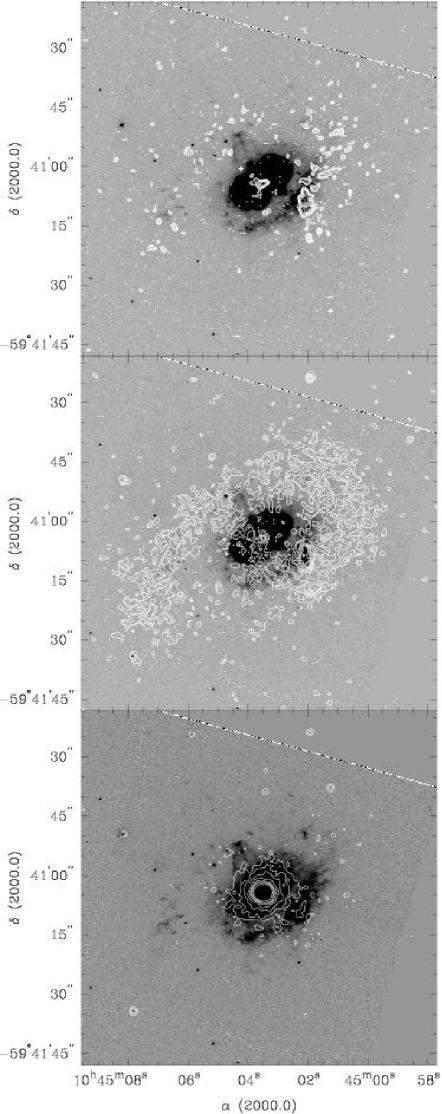
Figure 6: CHANDRA contours in the same energy bands as in in Fig. 4 are compared to an HST F658N image.

In several cases X-ray emission is found in areas where only very faint optical emission is present. This is especially true for the SS ridge and the parts of the W arc, the E rim (to the south) and the S ridge far from the central star. However, the large brightness differences between the fainter outer ejecta and the bright Homunculus make it hard to identify optical counterparts to these X-ray structures. For the E rim some faint optical emission is discernible even at the southernmost edge seen in X-rays. At the outermost parts of the W arc and S ridge (Fig. 6), however, no optical counterparts to the X-ray emitting material were detected.

The upper image in Fig. 6 shows the $0.2-0.6$ keV band and resembles the overlay of the nitrogen K line image. The nitrogen K lines are most prominent in the S condensation, parts of the S ridge and the W arc. Even though the central source also shows a maximum in this image, this maximum does not result from nitrogen line emission but rather from residuals of the continuum emission from the star.

The hard-band image shows X-ray emission from the central object. A small maximum in the S ridge however, turns out to be a real feature, after subtracting the CHANDRA PSF (Sect. 6.5).

4.2 CHANDRA Spectra

We extracted one spectrum from the entire “hook” (see Fig. 8) excluding the central source, and one spectrum for each region defined in Fig. 5. For comparison a spectrum of the central source was also extracted. The extraction area for the central source (see Fig. 8) was chosen to be as small as possible, to avoid overlap with the outer ejecta, but at the same time large enough to obtain a reasonable signal to noise ratio and to include most of the flux from the point source. Because of this, and because of photon pile-up, the flux of the central source is therefore underestimated.

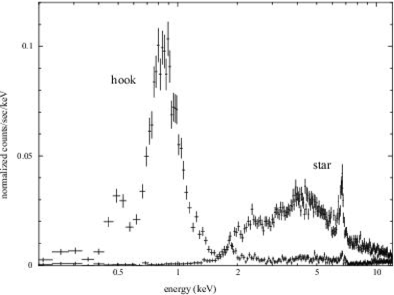
Figure 7: The X-ray spectrum of the “hook” compared with the spectrum extracted from the star. The total flux of the star is actually much higher than shown, since emission from only a small central region has been included in the extraction, and due to photon pile-up in the detector.

Fig. 7 shows the spectrum of the entire X-ray nebula and, for comparison, the spectrum of the central source. Because the temperature and compositions vary through the X-ray nebula, we did not attempt to model this spectrum.

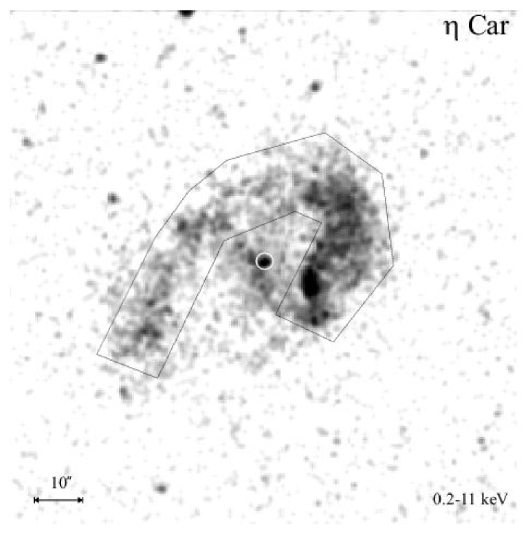
Figure 8: The CHANDRA image with the spectral extraction regions shown.

Fig. 7 shows the general features of the X-ray spectrum of the outer ejecta. The strongest emission is between 0.5 to 2 keV. The emission is mainly thermal – see also discussion later in the text – but only a few lines/line complexes are visible in this region. Between $0.4-0.55$ keV the larger bump, clearly separated from the continuous emission between 0.55 to 2 keV, is emission from the nitrogen K lines, as first noted in an ASCA observation by Tsuboi et al. (1997). The major contribution is from the N vii Ly_α lines at 0.50 and 0.49 keV (24.7792 and 24.7846 Å). A smaller fraction results from various N vi He_α lines around 0.43 keV (28.7870; 29.0843 and 29.5347 Å; see also Leutenegger et al. 2003). The high intensity of this blend of nitrogen lines indicates a nitrogen overabundance. This is consitent with the nebula of $\eta$ Carinae being CNO-processed material – which manifests itself in a higher nitrogen abundance (accompanied by oxygen and carbon underabundance, e.g. Davidson et al. 1982). In the softest region a second peak occurs around 0.3 keV which we tentatively identify with the Si xii Li_α lines at (40.9110 and 40.9510 Å). However, since the sensitivity and calibration is inferior in this energy band, and the resolution too low to seperate individual lines, this detection needs further confirmation. The spectrum of the hook also shows a peak around 1.8 keV, which is a blend of various Si-lines: Si xiii He_α (6.6479 Å) and Si xiv H_α (6.1804 and 6.1858 Å). Very likely also the Mg xii H_α (7.1058 and 7.1069 Å) lines contribute here. Above 2 keV, emission from the hook is barely visible. A more detailed discussion of the hard spectrum of the outer ejecta follows in Sect. 6.5.

The stellar spectrum itself is much harder and all emission below 1.8 keV is absorbed by the Homunculus nebula. Since the star is embedded in the dense nebula soft emission cannot penetrate to us, only the soft emission from the outer ejecta can reach us. Below 0.4 keV X-ray emission will also be heavily absorbed by the forground H i. The spectrum of the star is dominated by hard emission and the Fe K line complex.

Individual spectra for all areas defined in Fig. 5 have been extracted and are shown in Fig. 9. These plots range from 0.3 to 2 keV and the scale is again logarithmic. The range of the vertical axes are the same in each plot to visualize more easily intensity differences between each region. Fig. 9 also includes the model fits, which will be discussed later. Underneath each spectra the corresponding plot of the $\chi^{2}$ deviations of the model is indicated. We can seen that except for the intensity, the spectra are quite similar to each other and do not differ much from the overall spectrum of the total outer ejecta. Most of the X-ray emission lies between 0.6 and 1.2 keV. The emission from the nitrogen lines varies spatially, implying abundance variations by a factor of 5 through the outer emission.

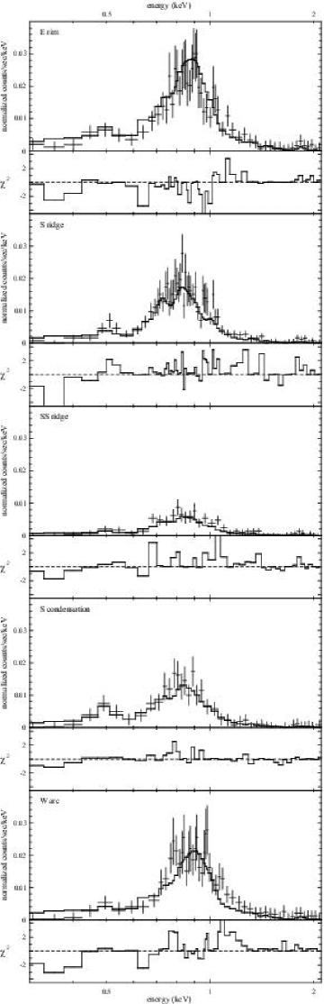
Figure 9: X-ray spectra extracted from select regions shown in Fig. 5). A collisionally ionized Mewe-Kaastra-Liedahl plasma emission model has been fitted to all spectra. We assume solar abundances for all elements except for nitrogen.

Each spectrum was fitted using the XSPEC analysis package and a Mewe-Kaastra-Liedahl thermal plasma model (e.g. Mewe et al. 1985, 1986) using the XSPEC spectral fitting software. This model includes line emissions from several elements and assumes coronal equilibrium. We used a foreground hydrogen column density of $\log N_{\rm H}$=21.3 (e.g. Savage et al. 1977). We adopted solar abundances for all elements with the exception of nitrogen, and kept the N abundance, temperature and emission measure as free parameters. We checked our model fits not only by inspection and minimization of the $\chi^{2}$ values but by comparing various other model fits to the data. Fits using Raymond-Smith plasma models yielded qualitatively acceptable results as well, though quantitatively, the deviations of the models from the spectra were somewhat larger. Bremsstrahlung models failed since no lines are included. This might also explain the large difference between our results and the temperature derived by Seward et al. (2001). Finally we also tested Mewe-Kaastra Liedahl models with a purely solar abundance for all elements and did not obtain any good fits.

Table 1 summarizes the results from each model fit to the spectra for each region. Temperatures are given in keV and K, along with the nitrogen abundance relative to solar abundance. Note that for the abundances we use the XSPEC convention which defines the abundance of a particular element as the number of nuclei per Hydrogen nucleus relative to solar abundances (Arnaud & Dorman 2002). In the last column the velocity of the shocking gas for the corresponding plasma temperatures are plotted. The shock velocities and gas temperature are related as T = v² (3$\mu$/16k) where v:= velocity of the shocking gas, T := post-shock temperature, k := Boltzman constant and $\mu$ := molecular weight (e.g. Landau & Lifschitz 1966, McKee 1987). With the temperature in keV one derives that v = 710$\sqrt{{\rm T}_{{\rm[keV]}}/\mu}$. The velocities in Table 1 have been calculated for different assumed values of the molecular weight: $\mu$=0.59 is for a completely ionized primordial hydrogen-helium mix of X=0.76 and Y=0.24, while $\mu$=0.67 results from a fully ionized gas with a mixture of X=0.6, Y=0.4. The contribution of higher metals can be neglected since they have no significant influence on the molecular weight. The latter ratio is in accordance with values derived for $\eta$ Carinae’s outer ejecta (Davidson et al. 1986). Table 1 shows that the velocities of the shocking gas for such a mixture of heavier and processed elements (predominantly more Helium) are reduced – roughly by 45 km s^-1 – compared to the velocities for a primordial gas mix. Both values for $\mu$ are given in this context to demonstrate the dependence of the post-shock temperatures on molecular weight. This is of interest, in particular, since theoretical models (García-Segura et al. 1996) for LBV nebulae predict values for the He abundance up to Y=0.76. This would increase the value of the molecular weight to as high as $\mu$=0.9 and similarly decrease the inferred velocities.

Table 1 shows that the W arc is the hottest region, followed by the E rim. The S ridge, SS ridge and S condensation show similar temperatures with the S ridge being slightly cooler. The nitrogen abundance is about 6 times solar on average if we exclude the S condensation, which has a derived nitrogen abundance of 22 relative to solar.

Table 1: Parameters of the models fitted to the individual spectra

Area	Temperature (keV)	Temperature (K)	Nitrogen	V (km s-1) / $\mu$=0.59	V (km s-1) / $\mu$=0.67
E rim	0.70$\pm$0.03 keV	8.0$\pm$0.4 106 K	8	773 km s-1	726 km s-1
S ridge	0.60$\pm$0.02 keV	7.0$\pm$0.2 106 K	6	710 km s-1	670 km s-1
SS ridge	0.63$\pm$0.04 keV	7.3$\pm$0.5 106 K	6	735 km s-1	690 km s-1
S condensation	0.63$\pm$0.04 keV	7.3$\pm$0.5 106 K	22	735 km s-1	690 km s-1
W arc	0.76$\pm$0.03 keV	8.8$\pm$0.4 106 K	4	807 km s-1	756 km s-1

5 Comparison of CHANDRA spectra and images with the kinematic data

As shown by Weis et al. (2001), the soft X-ray emission from the outer ejecta of $\eta$ Carinae is produced by shocks from fast moving structures. They showed that X-ray maxima, knots 1 & 2, correspond to regions where the fastest optical features are also located. In the following we compare the kinematic data with the CHANDRA images and spectra of each analogous region. In Fig.  10 the upper panel displays the contours of the CHANDRA image ($0.6-1.2$ keV) on the HST image and in the lower panel velocities in km s^-1 have been added. Blueshifted velocities are underlined and the font size of the characters increases with increasing velocities. With the higher resolution of the CHANDRA images we find in many cases an even better agreement between X-ray brightness and velocity. The brightest X-ray structures still are those with the highest velocities. The S condensation, for e.g., has velocities of 1290 to 1550 km s^-1 and in the SS ridge we find a 1260 km s^-1 feature. In the area of the W arc the expansion velocities are up to 1960 km s^-1. Note that Fig. 10 shows only the maximum velocities of each region for clarity; in reality each area actually spans a range of velocities (see Sect. 6.2).

For the best prediction of the X-ray luminosity and temperature, we have to weight the measured velocities with the densities of the gas. This is unfortunately not possible in a quantitative way using the present data. The echelle spectra do not include density sensitive lines, and an estimate from the H_α surface brightness (using emission measure and assuming a geometry) is not possible due to the overlap of the strong red- and blue-shifted [N ii] lines with H_α in the H_α filter band. Only few [S ii] based density estimates in the outer ejecta have been reported (Dufour et al. 1997, Weis 2002) and all are near the high density limit of the line diagnostic. A very rough qualitative estimate based on the surface brightness of the H_α line in the echelle spectra gives about 800 km s^-1. This is a typical gas velocity in the regions where we find the highest peak velocities (like the S ridge or W arc), which are often those having a very broad velocity distribution (up to at least 500 km s^-1; Weis & Duschl, in prep.). This raises the possibility of clump interactions. In most of the cases the highest velocity in a certain area implies a higher mean velocity in that region.

Due to stray light contamination from the bright central source, we cannot constrain the expansion velocities for the “bridge” region across the Homunculus. Also no measurements are available for the southern part of the E rim. However, one usable spectrum from this region indicated that expansion velocities as high as 1000 km s^-1 are present. This data-point has not been included on Fig.  10 since more measurements are needed for confirmation.

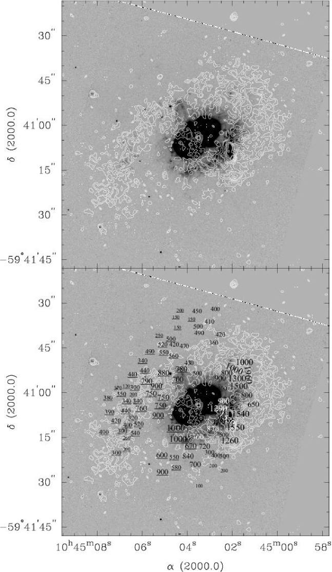
Figure 10: An overlay of the CHANDRA 0.6-1.2 keV image contours and our radial velocity measurements made with the 4 m Echelle Spectrograph on the optical F658N HST image (gray scale).

The shock velocities derived from the X-ray temperatures are listed in Table 1. Comparison with the radial velocity field based on our Echelle mapping shows that the typical velocities of the majority of the clumps are in agreement with the postshock temperatures from the fit to the X-ray spectra. The expansion velocities of the outer ejecta are therefore sufficiently high to explain the soft diffuse X-ray emission and the derived temperature of the gas.

The range of velocities detected in the outer ejecta field gives a natural explanation for the complexity of the X-ray spectra. In the areas which contain the highest velocities the velocity distribution of the clumps is generally also shifted to higher median velocities. The area, for instance, which contains the fastest expansion velocities (v$\sim$1900 km s^-1) – the W arc – shows the hardest X-ray spectrum (T=8.8 10⁶ K). Most of the clumps in this region have velocities between 700-900 km s^-1. These expansion velocities are in good agreement with those expected for a gas with that temperature (see Table 1).

The E rim also shows a relatively high temperature, T=8 10⁶ K, but the radial velocities are on average lower than in the W arc. However, the velocities detected (see Fig. 10) and the velocities derived from the X-ray spectra (see Table 1) are in good agreement. We also have to keep in mind that we measure only radial velocities so that the real expansion velocities are larger. For instance this is the case with the NN condensation and the NS condensation (which are actually part of the E rim as defined here). These structures show a radial velocity of about 700 km s^-1 but the tangential velocities are 1360 km s^-1 and 1180 km s^-1 for the NN and the NS condensation respectively (Walborn et al. 1978).

6 Discussions and conclusions

6.1 Origin of the X-ray nebula’s shape

The observed properties of the X-ray emission is a combination of the speed of the outflowing material and the density of the ambient medium into which the material is moving. The density of the ambient medium has to be sufficiently high to produce detectable emission.

Velocities of the warm gas are derived from our Echelle data supplemented by transverse velocities from proper motion measurements (Walborn et al. 1978). Densities of the ambient medium are derived from direct measurements using the [S ii] lines (Dufour et al. 1997, Meaburn et al. 1993), but for most of the gas we have to rely on emission measure derived from HST H_α images, which can be contaminated by red- or blueshifted [N ii] as previously discussed. While the absolute values for n${}_{e}^{2}$ is somewhat compromised by such contamination, the relative surface brightnesses still trace the relative overall column densities of the H ii gas.

With this information we have to understand why there is no strict correlation between the warm gas seen in the optical and the hot X-ray gas. There are two alternatives which might explain why the density is higher at the places which are X-ray bright.

The first possibility is an enhancement of density produced by an older stellar wind. During its main sequence phase, $\eta$ Carinae would have possessed a fast, low density wind which would have formed an interstellar bubble (Weaver et al. 1977). The interior of this bubble would be nearly evacuated since all material inside the bubble would be swept up to a radius of the order of 70 pc . As $\eta$ Carinae evolved into a blue supergiant and LBV, however, the wind velocity would decrease (down to several 100 km s^-1) and the mass loss rate would increase to 10${}^{-3}M_{\sun}yr^{-1}$ (e.g. Langer et al. 1994, García-Segura et al. 1996), which would increasingly fill the bubble with denser gas. After the “Great Eruption” the expansion of the outer ejecta into the remnants of this older, denser LBV wind (which at 0.35 pc has a density of roughly 150 times that of the ISM) would be able to slow down the ejecta to its current expansion velocity (Weis & Duschl, in prep) and could produce sufficient X-ray emission in the outer region of the nebula. Had this stellar wind been non-spherical, the ejecta would encounter the denser wind at different distances from the star.

Alternatively, higher densities may manifest localized regions in which the outer ejecta consists of many turbulent clumps which have different velocities. These clumps would collide into and over take each other, so the density is locally enhanced. This seems a reasonable explanation especially in the S condensation where a large number of clumps with different velocities are detected. X-ray emission is formed in regions with many clumps interacting with high velocities. In the E rim and outer regions of the S ridge fewer knots are detected and one might speculate that here the outer ejecta collides into the older stellar wind.

The Homunculus nebula itself is expanding at a velocity of 650 km s^-1 on average but is not visible in soft X-rays, though velocities this large should produce soft X-ray emission. The lack of detectable soft emission from the Homunculus is likely due to the low density (as judged from the low surface brightness in the H_α and N [ii] HST images) in the medium into which the Homunculus is expanding, which has been cleared out by earlier episondes of mass loss. Therefore the Homunculus expands practically freely and no shocks are formed.

6.2 Velocity fields and plasma temperatures

The ACIS-S spectra of the outer ejecta are decently fitted with single temperature coronal equilibrium models as we showed in sect. 4.2. Still, looking at the $\chi^{2}$ deviations, residual spikes are visible which indicate poorly fitted lines/line complexes. Indeed, several of these spikes correspond to lines complexes of e.g. Fe xvii and Fe xviii around 0.8 keV, Ne x and Ne ix at about 1.0 keV, Mg xi and Mg xii at about 1.3 keV and finally Si xiii and Si xiv at around 1.8 keV. While Doppler line velocity displacements are big enough to create noticeable shifts in several places in the outer ejecta , the highest velocity regions only represent a minor part of the total emission of the outer ejecta as seen in our Echelle spectra. Additionally, significant residuals are also visible in the X-ray spectra of regions without extremely fast moving knots. Therefore velocity offsets cannot fully explain the residuals. As traced by the Echelle data, we see not one typical expansion velocity but a distribution of velocities in all regions of the outer ejecta. Therfore we have different velocities which imply that the X-ray emission is composed of a distribution of emissivities, so that our single temperature fits are too simplistic.

The plasma properties we derive are therefore not the properties of the whole region, but rather the density weighted properties. We see the dominant emission component of a complex plasma, which is most probably also the reason why our single temperature fits are relatively good despite the multi-component and, due to the short timescales, non-equilibrium nature of the X-ray plasma in the outer ejecta (Weis et al. 2001). Our interpretation of the optical gas velocities as shock velocities rest on the details of the mass loss history of the LBV. The ejecta do not expand into a fast freely expanding wind as assumed by Leutenegger et al. (2003), but a dense very slow moving wind as explained above. The temperatures of the X-ray emitting gas are in good agreement with the velocity of the dominant emission component (weighted by surface brightness, therefore column density). What was missing is the very hot gas corresponding to the extremes of the velocities. This we may have found now with the ACIS data.

6.3 Missing X-ray emission from the NN bow

We detected soft X-ray emission from all the optical line emitting regions outside the Homunculus and the presumably low density envelope around it. Besides this region, there is one notable structure without X-ray emission: the NN bow. This roughly trapezoidal region is regarded as part of the outer ejecta and appears as a possible radial extension of the equatorial disk (Duschl et al. 1995). Surprisingly, the region is devoid of all soft emission, as can best be seen in the overlay of the soft X-ray emission on the HST WFPC2 F658N image (Fig. 10, middle panel). Since the radial velocities of the ionized gas belonging to the NN bow are typically around $-650$ km s^-1 (Meaburn et al. 1993, Weis et al. 2001) (similar to other regions of the outer ejecta), one would expect to see similar X-ray emission. The apparent minimum in the X-ray emission around the NN bow could be explained as a particularly deep X-ray shadow. The soft X-ray flux limit is as low as the one observed for the Homunculus itself. Assuming again shocks as the creation mechanism of the X-ray emission we would expect gas with a plasma temperature around 0.56 keV, and the total absence would point at an H i foreground density of about 10²² cm^-1, similar to the column density through the Homunculus. Still, since the gas in the NN bow is blueshifted, one would expect to see this gas on the front side of the dense gas. It appears therefore that the NN bow is expanding into a low density region. Nothing is stopping the expansion in line of sight, the density of the ambient medium is too low to create soft X-rays, and there are also – in contrast to the S condensation – no faster knots or clumps overtaking the slower gas in this region. At the northern end, however, shocks might form, and here at the optically bright NN condensation X-ray emission is present. It is further possible that X-ray emission behind the NN bow is absorbed by the NN bow itself. The only measurements of the density of the gas in the NN bow is a lower limit from [S ii] line ratios which as mentioned above are close to the high density limit (Dufour et al. 1997, Weis 2002). The density of the outer ejecta (outside the bright clumps) appears rather homogeneous (Weis et al., in prep.) with at least n${}_{e}\sim 10^{4}$ e^- cm^-3, consistent with the NN bow lower limit. For an assumed cylindrical geometry and size based on the observed dimensions in the HST images (diameter of the cylinder d=0.065 pc) we get therefore an absorbing column of at least $\sim 2\times 10^{22}$ cm^-2 through the NN bow. This is large enough to completely hide any $0.6$ keV plasma at the sensitivity of our data.

Another interpretation is that an X-ray shadow could be formed if the equatorial disk (Duschl et al. 1995) or its extension shadows the soft X-ray emission in the center and western part of the NN bow. In this scenario the expansion of the disk produces X-ray emitting shocks only at the outer edges, forming the bright X-ray rim at the NN condensation and the “bridge” (see also next section). Unfortunately, with the present data set details of the absorption and possible changes of the absorption across the NN bow cannot be derived due to a lack of X-ray photons. It is of interest to note that there is an X-ray bright spur just on the opposite side of the NN bow (the S condensation) which is spatially consistent with the plane of the equatorial disk.

Thus, both self absorption and/or expansion into low density environment can explain the lack of soft X-rays from the NN bow. Much deeper X-ray observations are needed to sort out the individual contributions of the processes.

6.4 The X-ray bridge across the Homunculus

In addition to the general lack of soft X-ray emission from the Homunculus region we can see in the CHANDRA data a “bridge” of soft emission crossing the Homunculus from the south-east to the north-west (see Fig. 3 and Fig. 10). We extracted a spectrum from this structure and find that it is rather similar to the X-ray spectra of the outer ejecta. A single temperature Mewe-Kaastra-Liedahl model as fitted to the other spectra (solar abundance except for nitrogen) gives an adequate fit to the data and yields a temperature of 0.67 keV and a nitrogen overabundance of a factor of 4. This is in good agreement with values found in other regions of the outer ejecta. The bridge has a somewhat lower X-ray surface brightness than most of the other regions in the outer ejecta (middle panel Fig. 4), but shows similar small scale variations in the surface brightness. It appears from all the properties as another part of the outer X-ray nebula.

The most straightforward interpretation for the soft X-ray bridge across the Homunculus is therefore a clump or a group of clumps located physically in front of the Homunculus, which was not seen in previous observations due to insufficient spatial and spectral resolution. The bridge is slightly below the optical disk and might represent shocks at the very outer ends of the disk, which in projection would appear offset from the bright optical emission of the disk. Unfortunately, the strong scattered light from the Homunculus prevents us from detecting related H_α emitting gas in our Echelle spectra and therefore determining the velocity field of this gas. In the HST images, any optical extension of the disk is also difficult to detect due to the very bright optical emission of the Homunculus.

6.5 Hard X-ray emission from the nebula around $\eta$ Carinae

We have shown in section 4.1 that some of the hard X-ray emission coinciding with the S condensation and the SS ridge are untouched by the PSF subtraction and therefore real. This implies that the S condensation and some of the SS ridge show hard emission, consistent with plasma temperatures comparable to the central source. The implied shock velocities are well in excess of 1500 km s^-1. Unfortunately the number of photons in both features are too small to generate a meaningful spectrum, but the result lends some support for the notion that not all of the hard tail and the Fe xxv visible in the total nebular spectrum (Fig.  7) are due to wings of the central source’s PSF, but intrinsic to the highest velocity knots in the nebula.

6.6 No X-rays from the strings

Some of the most puzzling features of the outer nebula are several extremely narrow optical emission filaments, dubbed “strings” (Weis et al. 1999), “whiskers” (Morse et al. 1998) or “spikes” (Meaburn et al. 1996). Because of their high velocity – nearly 1000 km s^-1 (Weis et al. 1999) – and large density – n${}_{e}\sim 10^{4}$ e^- cm^-3 (Weis 2002) it is worthwhile to search for X-ray emission from these structures. Detection of such emission would constrain the properties of the interaction of the “strings” with the surrounding medium and would further limit the possible creation mechanisms of these enigmatic features. The northwestern strings (#3 and #4 as designated in Weis et al. 1999) are located in the complex region of the W arc. Plenty of diffuse X-ray emission is present, but no emission can be convincingly associated with the strings. The southeastern strings are located in a much less crowded region. Unfortunately no diffuse X-ray emission can be seen either at the tip or along the body of the strings (#1, #2 and #5). The reason for this non-detection is most probably in the very small working surface of the strings (Weis et al., in prep.). Much deeper CHANDRA data will be needed to search for the interaction of the strings with the surrounding material.

7 Summary

With the new CHANDRA data we can conclude that the hook shape of the X-ray emission is not solely determined by the distribution of fast moving ejecta, as implied by Weis et al. (2001), but also by absorption of the soft X-rays and by the distribution of denser gas far from the Homunculus. The density enhancement could either be due to a remnant stellar wind and/or – as seen from the HST images and kinematics – from the mutual interaction of the outer ejecta with itself, which would yield the more patchy nebular structure due to the non-uniform distribution of the fast and slower moving gas knots. In general the detected velocities of the majority of the clumps in the outer ejecta are consistent with the velocities expected from the X-ray gas with temperature derived from the CHANDRA spectra, supporting the presence of a low velocity, dense LBV wind before the “Great Eruption”. This also naturally explains the missing X-ray emission of the expanding Homunculus. The surprising absence of diffuse X-rays from the NN bow can be explained by its nearly freely expansion in line of sight. Only at the northern tip – the “NN condensation” – an X-ray bright spot is visible; this may be indication of shocked emission. As a second possibility the NN bow could be the outer part of a dense expanding equatorial disk as proposed by Duschl et al. (1995) which shadows parts of the NN bow in X-rays so only the rim of the disk which forms shocks is visible in X-rays as the bridge and the bright rim of the NN bow.

The X-ray spectra are well approximated by single temperature collisional equilibrium models assuming solar abundances for all elements except nitrogen. The N abundance is strongly enhanced, consistent with the optical spectra (Dufour et al. 1997), earlier ASCA (Tsuboi et al. 1997), CHANDRA (Seward et al. 2001, Weis et al. 2001), and XMM-Newton results (Leutenegger et al. 2003) and the notion of $\eta$ Carina being a very massive evolved star (but for a different interpretation see e.g.  Leutenegger et al. 2003). We found indications of very hot gas due to fast shocks and detected a previously unseen cloud of soft X-ray emitting gas in front of the Homunculus, most probably another cloud in the outer ejecta. This cloud underlines the 3d structure of the outer ejecta and that the apparent hook shape of the X-ray nebula is only a complex mirage due to projection, absorption and true density inhomogeneities.

- (1) Arnaud, K., & Dorman, B. 2002, XSPEC User’s Guide for version 11.2.x, NASA
- (2) Chlebowski, T., Seward, F. D., Swank, J., & Szymkowiak, A. 1984, ApJ, 281, 665
- (3) Corcoran, M. F., Rawley, G. L., Swank, J. H., Petre, R. 1995, ApJ, 445, 121
- (4) Corcoran, M. F., Ishibashi, K., Swank J.H., Petre, R. 2001a, ApJ, 547, 1034
- (5) Corcoran, M. F., Ishibashi, K., Swank J.H., et al. 2001b, ApJ, 562, 1031
- (6) Damineli, A. 1996, ApJL, 460, 49
- (7) Damineli, A., Conti, P. S., & Lopes, D. F. 1997, New Astronomy 2, 107
- (8) Davidson, K., Walborn, N. R., & Gull, T. R. 1982, ApJ, 254, L47
- (9) Davidson, K., Dufour, R. J., Walborn, N. R., & Gull, T.R. 1986, ApJ, 305, 867.
- (10) Davidson, K., & Humphreys, R. M. 1997, ARA&A, 35, 1
- (11) Dufour, R. J., Glover, T. W., Hester, J. J., Currie, D. G., van Orsow, D., & Walter, D. K. 1997, Luminous Blue Variables: Massive Stars in Transition. ASP Conference Series, Vol. 120, ed. A., Nota and H., Lamers, p.255
- (12) Duschl, W. J., Hofmann, K.-H., Rigaut, F., & Weigelt, G. 1995, RevMexAA SdC, 2, 41
- (13) García-Segura, G., Mac Low, M.-M., & Langer, N. 1996, A&A, 305, 229
- (14) Gaviola, E. 1946, RevAstron, 18, 252
- (15) Gaviola E. 1950, ApJ 111, 408
- (16) Herschel, J. F. W. 1847, Results of Astronomical Observations Made During the Years 1834-1888 at the Cape of Good Hope, London, 32
- (17) Hillier, D. J., Davidson, K., Ishibashi, K., & Gull, T. 2001, ApJ, 553, 837
- (18) Humphreys, R. M. 1999, Lecture Notes in Physics Vol. 523, 243, Springer-Verlag, ISBN 3-540-65702-9
- (19) Humphreys, R. M., & Davidson, K. 1979 ApJ, 232, 409
- (20) Humphreys, R. M., & Davidson, K. 1994, PASP, 106, 1025
- (21) Humphreys, R. M., Davidson, K., & Smith, N. 1999, PASP, 111, 1124
- (22) Innes, R. T. A. 1903, Cape Ann. 9, 75B
- (23) Ishibashi, K., Corcoran, M. F., Davidson, K., et al. 1999, ApJ, 524, 983
- (24) Landau, L. D., & Lifschitz, E. M. 1966, Lehrbuch der theoretischen Physik, Hydrodynamik, Berlin: Akademie-Verlag
- (25) Langer, N., Hamann, W.-R., Lennon, M., et al. 1994 A&A, 290, 819
- (26) Leutenegger, M. A., Kahn, S. M., & Ramsay, G. 2003, ApJ, 585, 1015
- (27) McKee, C. F. 1987 Spectroscopy of astrophysical plasmas, Cambridge and New York, Cambridge University Press, p. 226-254.
- (28) Meaburn, J., Gehring, G., Walsh, J. R., Palmer, J. W., Lopez, J. A., Bryce, M., & Raga, A. C. 1993, A&A, 276, L 21
- (29) Meaburn, J., Boumis, P., Walsh, J. R., Steffen, W., Holloway, A. J.; Williams, R. J. R., & Bryce, M. 1996, MNRAS, 282, 1313
- (30) Mewe, R., Gronenschild, E. H. B. M., & van den Oord, G. H. J. 1985, A&AS, 62, 197
- (31) Mewe, R., Lemen, J. R., & van den Oord, G. H. J. 1986, A&AS, 65, 511
- (32) Morse, J. A., Davidson, K., Bally, J., et al. 1998, AJ, 116, 2443
- (33) Nota, A., Livio, M., Clampin, M., & Schulte-Ladbeck, R. 1995, ApJ, 448, 788
- (34) Pittard, J. M., & Corcoran, M. F. 2002, A&A, 383, 636
- (35) Savage, B. D., Drake, J. F., Budich, W., & Bohlin, R. C. 1977, 216, 291
- (36) Seward, F. D., & Chlebowski, T. 1982, ApJ, 256, 530
- (37) Seward, F. D., Butt, Y. M., Karovska, M., Prestwich, A., Schlegel, E. M., & Corcoran, M. F. 2001, ApJ, 553, 832
- (38) Thackeray, A. D. 1949, Obs, 69, 31
- (39) Thackeray, A. D. 1950, MNRAS, 110, 524
- (40) Thackeray, A. D. 1961, Observatory, 81, 99
- Tsuboi, Koyama, Sakano, & Petre (1997) Tsuboi, Y., Koyama, K., Sakano, M., & Petre, R. 1997, PASJ, 49, 85
- (42) van Genderen, A. M., & Thé, P. S. 1984, SpaceSciRev, 39, 317
- (43) Viotti, R. 1995, RevMexAA SdC, 2, 10
- (44) Walborn, N. R., Blanco B. M., & Thackeray, A. D. 1978, ApJ, 219, 498
- (45) Walborn, N. R. 1976, ApJL, 204, L17
- (46) Weaver, R., McCray, R., Castor, J., Shapiro P., & Moore, R. 1977, ApJ, 218, 377
- (47) Weis, K. 2001a, Reviews in Modern Astronomy 14, ed.: Schielicke R.E., Springer-Verlag, ISBN 3-9805176-4-0, 261 and astro-ph/0104214
- (48) Weis, K. 2001b, ASP Conf. Series Vol. 242, 129
- (49) Weis, K. 2002, B. Balick (ed.), ETA CARINA WORKSHOP, 10-13 July 2002, Mt. Rainier WA, Eta Car: Reading the Legend, Online-proceedings, http://www.astro.washington.edu/balick/eta_conf/eta_talks_posters.html and astro-ph/0208493
- (50) Weis, K., Duschl, W. J., & Chu, Y.-H. 1999, A&A, 349, 467
- (51) Weis, K., Duschl, W. J., & Bomans, D. J. 2001, A&A, 367, 566