Radiative Shock-Induced Collapse of Intergalactic Clouds

Abstract

Accumulating observational evidence for a number of radio galaxies suggests an association between their jets and regions of active star formation. The standard picture is that shocks generated by the jet propagate through an inhomogeneous medium and trigger the collapse of overdense clouds, which then become active star-forming regions. In this contribution, we report on recent hydrodynamic simulations of radiative shock-cloud interactions using two different cooling models: an equilibrium cooling-curve model assuming solar metallicities and a non-equilibrium chemistry model appropriate for primordial gas clouds. We consider a range of initial cloud densities and shock speeds in order to quantify the role of cooling in the evolution. Our results indicate that for moderate cloud densities ($\gtrsim 1$ cm^-3) and shock Mach numbers ($\lesssim 20$), cooling processes can be highly efficient and result in more than 50% of the initial cloud mass cooling to below 100 K. We also use our results to estimate the final H₂ mass fraction for the simulations that use the non-equilibrium chemistry package. This is an important measurement, since H₂ is the dominant coolant for a primordial gas cloud. We find peak H₂ mass fractions of $\gtrsim 10^{-2}$ and total H₂ mass fractions of $\gtrsim 10^{-5}$ for the cloud gas, consistent with cosmological simulations of first star formation. Finally, we compare our results with the observations of jet-induced star formation in “Minkowski’s Object,” a small irregular starburst system associated with a radio jet in the nearby cluster of galaxies Abell 194. We conclude that its morphology, star formation rate ($\sim 0.3M_{\odot}$ yr^-1) and stellar mass ($\sim 1.2\times 10^{7}M_{\odot}$) can be explained by the interaction of a $\sim 9\times 10^{4}$ km s^-1 jet with an ensemble of moderately dense ($\sim 10$ cm^-3), warm ($10^{4}$ K) intergalactic clouds in the vicinity of its associated radio galaxy at the center of the galaxy cluster.

1 Introduction

Combined optical and radio observations of a number of extragalactic radio jets in both low-luminosity (FRI) and high-luminosity (FRII) galaxies have revealed interesting correlations between the jets and apparent regions of active star formation. One of the first objects demonstrated to show such a correlation was the nearest radio galaxy, Centaurus A (e.g. Blanco et al., 1975). Other examples have been found as the sensitivity and spatial resolution of radio and optical telescopes has improved. In the case of Centaurus A, recent observations with the Hubble Space Telescope, when compared to radio images obtained with the Very Large Array, have confirmed that there are about half a dozen young ($<15$ Myr) OB associations near filaments of ionized gas located between the radio jet and a large H I cloud (Mould et al., 2000; Rejkuba et al., 2002). Another nearby example is “Minkowski’s Object,” a peculiar small starburst system at the end of a radio jet emanating from the elliptical galaxy NGC 541, located near the center of the cluster of galaxies Abell 194 (van Breugel et al., 1985). Star forming regions associated with radio sources have also been found in cooling flow clusters (McNamara, 2002).

Correlations between radio and optical emissions have also been observed in the so-called “alignment effect” in distant ($z>0.6$) radio galaxies (Chambers, Miley, & van Breugel, 1987; McCarthy et al., 1987). The best studied example here is 4C41.17 at $z=3.8$, where deep spectroscopic observations have shown that the bright, spatially extended, rest-frame UV continuum emission aligned with the radio axis of this galaxy is unpolarized and shows P Cygni-like features similar to those seen in star-forming galaxies (Dey et al., 1997).

Collectively, these observations are most compellingly explained by models in which shocks generated by the radio jet propagate through an inhomogeneous medium and trigger gravitational collapse in relatively overdense regions (Begelman & Cioffi, 1989; De Young, 1989; Rees, 1989). A detailed analysis of the jet-induced star formation in 4C41.17 has been presented by Bicknell et al. (2000). In that object, Hubble Space Telescope images showed a bimodal optical continuum structure parallel to the radio jet (van Breugel et al., 1999), strongly supporting the idea that the star formation was triggered by sideways shocks.

Although the analytic arguments in favor of this model are compelling, the complex nature of this problem, including nonlinear effects from higher-order coupling between hydrodynamics, cooling, and gravity, suggest that numerical studies may provide a more complete and detailed picture. Furthermore, numerical studies allow us to probe environments that may be observationally out of reach. For example, such studies may be able to parameterize the conditions of shock-induced star formation in the early universe, where direct observations of star-forming regions are not possible. This could be important to understanding the role of jets in the feedback of active galactic nuclei (AGN) on their environment. Numerical simulations also give us insight into the role of shock-induced star formation in other environments such as supernova shocks and cloud-cloud collisions.

The interaction of a strong shock with a single, non-radiative cloud has been the subject of many numerical studies. A thorough analysis of this problem and a review of relevant literature is provided by Klein, McKee, & Colella (1994). A more recent study, considering the interaction of a strong shock with a system of clouds, is presented by Poludnenko, Frank, & Blackman (2002). For a non-radiative cloud the passing shock ultimately destroys the cloud within a few dynamical timescales. Destruction results primarily from hydrodynamic instabilities at the interface between the cloud and the post-shock background gas.

Less well studied is the case of a strong shock interacting with a radiative cloud. Mellema, Kurk, & Röttgering (2002) showed that the effects of a shock on such a cloud are very different from the non-radiative case. Instead of re-expanding and quickly diffusing into the background gas, the compressed cloud instead breaks up into numerous dense, cold fragments. These fragments survive for many dynamical timescales and are presumably the precursors to star formation.

In this work, we extend previous numerical studies by considering two primary cooling models. The first model uses an equilibrium cooling curve with a tunable metallicity, set to solar in this work. As such, this model provides a reasonable approximation for cooling in metal-enriched clouds around low-redshift (FRI) radio galaxies. The second model solves the full non-equilibrium chemistry for a primordial gas mixture. This model is very well suited to address jet-induced star formation in pristine clouds around high-redshift (FRII) galaxies. With both models we explore a substantial subset of the parameter space over which shock-induced star formation may apply. We proceed in § 2 by discussing the relevant physical processes, the timescales over which they act, and the limitations of the present study. The numerical methods and models employed in the current work are discussed in § 3, and the results of the models are presented in § 4. Further implications for star formation are discussed in § 5. Our conclusions are briefly recapped in § 6.

2 Shock-Cloud Interactions

The basic idea of shock-induced star-formation is relatively simple. A strong shock passes through a clumpy medium, triggering many smaller-scale compressive shocks in overdense clumps. These shocks increase the density inside the clumps and make it possible for them to radiate more efficiently. If the radiative efficiency of the gas has a sufficiently shallow dependence upon the temperature, then radiative emissions are able to cool the gas rapidly, in a runaway process, producing even higher densities as the cooling gas attempts to re-attain pressure balance with the surrounding medium (Field, 1965; Murray & Lin, 1989). Both the reduction in temperature and the increase in density act to reduce the Jeans mass, above which gravitational forces become important. Any clump that was initially close to this instability limit will be pushed over the edge and forced into gravitational collapse. Thus, the passing of a shock through a clumpy medium may trigger a burst of star formation. Several processes, acting on different timescales as discussed below, govern whether or not cooling and star formation are able to proceed.

2.1 Jet-Cloud Collision

In this work we are primarily interested in the interactions occurring over a relatively small region of a much larger intergalactic environment. However, since this work is being presented in the context of jet-induced star formation we wish to first motivate our treatment of the problem as either a single or a few overdense clumps being overrun by a planar shock. The presumption that the intergalactic medium is clumpy and multi-phase with a range of densities and temperatures is consistent with observational and theoretical studies of such objects as high-pressure ($10^{5}$ K cm^-3) cooling flow clusters (Ferland, Fabian, & Johnstone, 2002) and the giant emission-line halos found around distant radio galaxies (Reuland et al., 2003). The planar-shock assumption is also consistent, although the specific relation between the shock and the jet may vary somewhat from system to system.

For luminous FRII galaxies, with their powerful relativistic jets, it is unlikely that star formation will occur within the stream of the jet itself. More likely, star formation will proceed within a cocoon of shock gas around the jet (Begelman & Cioffi, 1989; De Young, 1989; Rees, 1989). Because of the very large sizes of these cocoons, the triggering shocks will appear to be nearly planar over the length scales considered in this study.

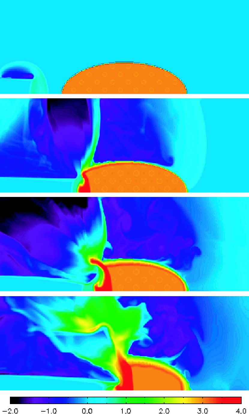
For low-luminosity FRI galaxies, the jets have a lower Mach number and appear turbulent; no hotspots or cocoons form (Bicknell, 1984). Nevertheless, such jets may still trigger potential star-forming shocks through collisions with nearby clouds, as illustrated in the following numerical simulation. This simulation is performed using the Cosmos code described in § 3 below. Our parameters are chosen to closely resemble the conditions of Minkowski’s Object, the small starburst system at the end of the radio jet emanating from the radio galaxy NGC 541. Specifically, we set up an elliptical cloud with a major axis of 10 kpc, a minor axis of 5 kpc, a temperature $T=10^{6}$ K, and density $n_{cl}=0.1$ cm^-3. This corresponds to an initial cloud mass of $\approx 10^{9}M_{\odot}$.

The radio source associated with NGC 541 is of relatively low luminosity and exhibits a FRI-type morphology (Fanaroff & Riley, 1974). We, therefore, used the detailed radio and X-ray study of the proto-typical FRI-type radio galaxy 3C31 by Laing & Bridle (2002) to estimate plausible jet parameters near Minkowski’s Object, at $\sim 15$ kpc from the NGC 541 AGN. For our numerical simulations, we assume that the long axis of the cloud is aligned with a jet of high velocity ($9\times 10^{4}$ km s^-1), low density ($10^{-4}$ cm^-3), hot ($10^{9}$ K) gas flowing onto our computational grid. The diameter of the jet nozzle is equal to half the diameter of the cloud along the minor axis. The assumption of an elliptical cloud is not essential to this discussion, although it can be easily motivated by tidal stretching from the nearby galaxies. It is also not essential that the jet be aligned with the long axis of the cloud, although this is convenient for numerical purposes.

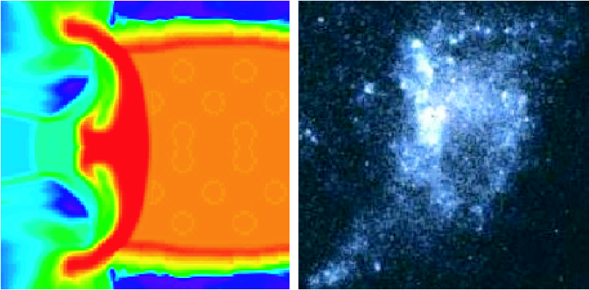
As shown in Figure 1 the jet-cloud collision triggers a nearly planar shock down the long axis of the cloud. As the bow shock from the jet wraps around the cloud, it also triggers shocks along the sides of the cloud. A similar shock structure may explain the filamentary nature of the star-forming region in Minkowski’s Object. Note the similarities between the next-to-last frame of the numerical simulations and the observations as illustrated in Figure 2.

We stress that this simulation is only intended to motivate our subsequent treatment of the problem at much smaller physical scales. This simulation is unable to resolve the many moderately dense ($\sim 10$ cm^-3), warm ($10^{4}$ K) sub-kiloparsec clouds presumed to be interspersed within the larger cloud simulated here. Further, the jet is not fully evolved when it hits the cloud, although this may not be critical since even a fully-evolved jet would trigger shocks in any clouds that crossed its path.

2.2 Timescales

The initial conditions for all of our subsequent calculations consist of a spherical cloud of radius $R_{cl}$ and density $\rho_{cl}=m_{H}n_{cl}$ in initial pressure equilibrium with a background gas at temperature $T_{b,i}$ and density $\rho_{b,i}=m_{H}n_{b,i}=\rho_{cl}/\chi<\rho_{cl}$, where $\chi>1$ is the density ratio between the cloud and background gases. Given this simplified geometry and parameterization, a number of useful dynamical timescales can be estimated analytically in order to weigh the relative importance of various physical effects including: shock crossing, shock compression, instability growth, cooling, freefall, magnetic acceleration, and thermal conduction.

The first timescale of interest is the shock-passage time. A planar shock of velocity $v_{sh,b}$ measured in the background gas, passes over the cloud in a time

$$t_{sp}=\frac{2R_{cl}}{v_{sh,b}}~{}.$$ (1)

The gas in the cloud will react to the shock on roughly a sound-crossing time

$$t_{sc}=\frac{2R_{cl}}{c_{s,cl}}~{},$$ (2)

where $c_{s,cl}$ is the initial isothermal sound speed of the gas in the cloud. Provided $c_{s,cl}\ll v_{sh,b}$, the cloud will rapidly find itself in an overpressure region and a nearly spherical shock will be driven into the cloud. The velocity of this shock can be estimated by assuming pressure equilibrium between the post-shock cloud material and the shocked background region. If the shock in the background is strong ($\mathcal{M}=v_{sh,b}/c_{s,b}\gg 1$), then the post-shock pressure is approximately equal to $\rho_{b,i}v_{sh,b}^{2}$. Similarly, the post-shock pressure in the cloud is of order $\rho_{cl}v_{sh,cl}^{2}$. Equating these, we estimate the velocity of the shock in the cloud as

$$v_{sh,cl}\simeq\left(\frac{\rho_{b,i}}{\rho_{cl}}\right)^{1/2}v_{sh,b}=\frac{v_{sh,b}}{\chi^{1/2}}~{}.$$ (3)

[More rigorous estimates are presented in Sgro (1975) and Klein, McKee, & Colella (1994).] This shock will compress the cloud on a timescale of approximately

$$t_{cc}=\frac{R_{cl}}{v_{sh,cl}}\simeq\chi^{1/2}\frac{R_{cl}}{v_{sh,b}}~{}.$$ (4)

This is an important dynamical timescale for the cloud.

After the shock has passed over it, the cloud becomes susceptible to both Rayleigh-Taylor and Kelvin-Helmholtz instabilities. The growth of the Rayleigh-Taylor instability is due to the acceleration of the cloud by the post-shock background gas. The acceleration timescale is the amount of time it takes to accelerate the cloud gas to the velocity of the post-shock background. If we consider the momentum transfer from a column of post-shock background gas with velocity $v_{b,ps}$ and cross-sectional area $\pi R_{cl}^{2}$ to a spherical cloud, then the acceleration timescale is given roughly by $t_{acc}\approx\chi R_{cl}/(3v_{b,ps})$, where we have assumed a mean post-shock force acting on the cloud of $\pi R_{cl}^{2}\rho_{b,ps}v_{b,ps}^{2}$ and used the shock-jump condition $\rho_{b,ps}=4\rho_{b,i}$ with an adiabatic index of $\Gamma=5/3$. The shock-jump conditions also give us $v_{b,ps}=3v_{sh,b}/4$. Thus, the acceleration timescale can be rewritten as

$$t_{acc}\approx\chi\frac{R_{cl}}{v_{sh,b}}\approx\chi^{1/2}t_{cc}~{},$$ (5)

where we have dropped a numerical factor of order unity. This gives an acceleration of $g\sim v_{sh,b}/t_{acc}\sim R_{cl}/t_{cc}^{2}$, corresponding to a Rayleigh-Taylor growth time of $t_{RT}^{-1}\simeq(gk)^{1/2}$ for a perturbation of wavenumber $k$ (Chandrasekhar, 1961). Written in terms of the cloud-compression timescale, $t_{cc}$, the Rayleigh-Taylor growth time is

$$t_{RT}\sim\frac{t_{cc}}{(kR_{cl})^{1/2}}~{}.$$ (6)

Although the shortest wavelengths ($\lambda\ll R_{cl}$) have the fastest growth rates, they also saturate rapidly when their amplitudes $A\approx\lambda\ll R_{cl}$. Wavelengths corresponding to $kR_{cl}\sim 1$ are therefore the most disruptive. Hence, Rayleigh-Taylor instabilities will break up the cloud over a timescale comparable to the cloud compression.

For $\chi\gg 1$ the timescale for growth of the Kelvin-Helmholtz instability is $t_{KH}^{-1}=kv_{rel}/\chi^{1/2}$ (Chandrasekhar, 1961), where $v_{rel}$ is the relative velocity between the post-shock background and the cloud. Since the cloud accelerates rather slowly for $\chi\gg 1$, the relative velocity is approximately equal to the post-shock velocity of the background gas $v_{b,ps}=3v_{sh,b}/4$. Again, in terms of the cloud-compression timescale $t_{cc}$ , we have

$$t_{KH}\sim\frac{t_{cc}}{(kR_{cl})}~{}.$$ (7)

The Kelvin-Helmholtz instability will thus also act on a cloud-compression timescale.

The timescales above have been derived assuming adiabatic evolution of the gas and would be modified somewhat if radiative cooling were taken into account. However, our primary purpose is to roughly characterize some general timescales for these clouds, for which the values derived above are more than adequate.

If the cloud is not able to cool radiatively, then the above results suggest that the cloud will be destroyed over a time comparable to the cloud-compression timescale. This has been shown to indeed be the case in numerous hydrodynamic simulations (e.g. Klein, McKee, & Colella, 1994; Poludnenko, Frank, & Blackman, 2002). Destruction is enhanced by the fact that, after the compressive shock passes through itself and exits at the opposite surface of the cloud, it triggers a rarefaction wave traveling back into the cloud. This causes the cloud to re-expand and increases the pressure contrast between the compressed cloud and the post-shock external gas, effectively accelerating the growth of destructive instabilities.

However, if the cooling timescale is short compared to the cloud-compression timescale ($t_{cool}\ll t_{cc}$), a very different outcome is reached, as was shown in Mellema, Kurk, & Röttgering (2002). Cooling instabilities in the post-shock cloud material cause it to collapse into a very thin, cold dense shell behind the shock. This greatly enhances the density contrast between the post-shock cloud and background gases, which slows the growth of destructive instabilities. We can estimate the cooling timescale as

$$t_{cool}=\frac{1.5n_{cl,ps}k_{B}T_{cl,ps}}{(n_{cl,ps})^{2}\Lambda(T)}~{},$$ (8)

where the numerator is the energy density of the gas and the denominator is the volume emissivity. To get a general estimate of the cooling timescale, we use the approximate cooling rate, $\Lambda=1.33\times 10^{-19}T^{-1/2}$ erg cm³ s^-1 from Kahn (1976), appropriate for gas temperatures ranging from $5\times 10^{4}-5\times 10^{7}$ K. Applying the shock-jump conditions, the cooling timescale can be rewritten as

$$t_{cool}=C\frac{v_{sh,b}^{3}}{\chi^{3/2}\rho_{cl}}~{},$$ (9)

where $C=7.0\times 10^{-35}$ g cm^-6 s⁴. In this study we will predominantly explore the cooling-dominated regime $t_{cool}<0.1t_{cc}$. (A version of this condition is given in Mellema, Kurk, & Röttgering (2002), Eq. 1.) For our typical data with cloud radius $R_{cl}=100$ pc and density ratio $\chi=10^{3}$, we find that cooling will generally govern evolution for moderate cloud densities and shock velocities. However, sufficiently high shock velocities can suppress the effect of cooling over the cloud destruction time (e.g., for shock velocities $v_{sh,b}>10^{4}$ km s^-1 with $n_{cl}\leq 1$ cm^-3). Cooling is also negligible at sufficiently low densities (e.g., clouds with $n_{cl}<10^{-4}$ cm^-3 do not cool for $v_{sh,b}\geq 10^{3}$ km s^-1).

2.3 Limitations

Our models are subject to some limitations. Due to resolution requirements and computational limitations, the models have been studied in two-dimensional, Cartesian geometry, and so the clouds represent slices through infinite cylinders. As can be seen in the models presented below, the initial compressions are highly symmetric, and so the additional convergence expected in three-dimensional models might well lead to stronger compressions and enhanced cooling, especially for the primordial clouds which rely upon the formation of H₂. Three-dimensional simulations would also provide an additional degree of freedom for fragmentation through dynamical instabilities. Such models might, therefore, be expected to lead to the formation of greater numbers of fragments than seen below.

In all but one of our models, self-gravity is neglected, due to the geometry; self-gravity in cylindrical symmetry is noticeably different than in spherical symmetry. The relevant timescale for self-gravity is the free-fall timescale of the gas, $t_{ff}=(3\pi/32G\rho)^{1/2}$. The initial overdense clumps considered here are specifically chosen not to be self-gravitating, and the corresponding freefall time is long compared to other relevant timescales. However, as the clouds compress, the local free-fall timescale becomes significantly shorter. For most of the runs, self-gravity is just becoming important around the time we stop the simulations. In order to explore the effects of self-gravity, we include one run which solves for the self-gravity of the cloud. The results of that model indicate that the inclusion of self-gravity would likely enhance compressions and cooling in all of the models.

Examining three dimensional models with self-gravity, at comparable resolution to that used in the models presented here, will require the implementation of adaptive mesh refinement to concentrate resolution only over those regions which form dense fragments. That capability is currently being added to the code described below, and results will be presented in future work.

If the background medium is magnetized, then magnetic field lines can become trapped in deformations on the surface of the cloud. As these field lines are stretched, the magnetic pressure along the leading edge of the cloud can increase enough to accelerate the disruption of the cloud through the Rayleigh-Taylor instability (Gregori et al., 1999). We can estimate the importance of this effect by accounting for the increased acceleration of the cloud due to magnetic pressure (Gregori et al., 1999)

$$g=\frac{\rho_{b,i}v_{sh,b}^{2}+P_{B}}{R_{cl}\rho_{cl}}~{},$$ (10)

where $P_{B}=B^{2}/8\pi\equiv P_{b,ps}/\beta$. The Rayleigh-Taylor growth time $t_{RT}^{-1}\simeq(gk)^{1/2}$ now becomes

$$t_{RT}\sim\frac{t_{cc}}{\{[1+3/(4\beta)]kR_{cl}\}^{1/2}}~{}.$$ (11)

From this estimate we see that, even for strong magnetic fields ($\beta\lesssim 10$), the Rayleigh-Taylor growth time remains comparable to the cloud-compression timescale and hence longer than the cooling timescales for most of the runs considered.

Tangled magnetic fields within the clouds would also act to resist compression, potentially reducing cooling, and enhancing cloud destruction by shocks. We are currently working to add MHD capabilities to our numerical code, and shall examine the effects of realistic magnetic field strengths in future work.

If thermal conduction is important then the cloud will evaporate into the hot background medium. The rate at which the cloud evaporates can be written (Klein, McKee, & Colella, 1994)

$$\dot{M}_{cl}=4\pi R_{cl}^{2}\rho c_{s}F(\sigma_{0})~{},$$ (12)

where $\sigma_{0}$ is the saturation parameter and $F(\sigma_{0})$ is a dimensionless quantity of order unity. If we define an ablation timescale $t_{ab}\equiv M_{cl}/\dot{M}_{cl}$, then in the post-shock environment

$$t_{ab}\approx\frac{\chi^{1/2}t_{cc}}{7F(\sigma_{0})}~{}.$$ (13)

We see that for $\chi\gtrsim 10^{2}$, the ablation timescale will be comparable to or longer than the compression timescale. Thus, for the parameters considered in this study, thermal conduction can safely be ignored.

3 Numerical Methods

The numerical calculations discussed below have been computed using Cosmos, a massively parallel, multidimensional, radiation-chemo-hydrodynamics code designed for both Newtonian and relativistic flows developed at Lawrence Livermore National Laboratory. The relativistic capabilities and tests of Cosmos are discussed in Anninos & Fragile (2003). Tests of the Newtonian hydrodynamics options and of the microphysics relevant to the current work are presented in Anninos, Fragile & Murray (2003), and so we shall not discuss those in detail here. The calculations are carried out on a fixed, two-dimensional Cartesian ($x$,$y$) grid, implying that the simulated clouds are cylindrical rather than spherical. This limitation is currently necessary in order to maintain sufficient resolution to follow the fragmentation of the clouds.

3.1 Cooling Models

All of the remaining results presented here were performed at a fixed spatial resolution of $0.5\times 0.5$ pc per zone. There are 200 zones across the initial radius of the cloud, consistent with the resolution requirements suggested by Klein, McKee, & Colella (1994). We note, however, that in the presence of cooling, which leads to even higher densities, the resolution requirements become even more stringent. We find that we are only able to reliably follow the fragmentation of the cloud for slightly longer than the cloud-compression timescale, $t_{cc}$. Beyond that point, further compression of the cloud is prevented by numerical resolution rather than any physical mechanism. We have allowed a few of our runs to evolve for longer times (on the order of a few $t_{cc}$) to confirm that the cold, dense cloud fragments which form are relatively long lived, consistent with the findings of Mellema, Kurk, & Röttgering (2002). Further study of the evolution of these dense fragments will require finer resolution or an adaptive mesh.

3.1.1 Equilibrium Cooling Curve - Low Redshift Systems

Two radiative cooling and heating models are considered in this study. In the first model, appropriate for enriched clouds around low-redshift galaxies, local cooling is given by the following cooling function:

$$\Lambda(T,n)=\left[\sum_{i}\dot{e}_{i}(T)(f_{I}n)^{2}+\dot{e}_{M}(T)f_{M}n^{2}+Jn\right]\times\left\{\begin{array}[]{ll}\exp[(T-T_{min})/\delta T]&\mbox{if}~{}T\leq T_{min},\\ 1&\mbox{otherwise},\end{array}\right.$$ (14)

based in part on an equilibrium (hydrogen recombination and collisional excitation) cooling curve. Here $\dot{e}_{i}$ is the cooling rate from hydrogen and helium lines, $\dot{e}_{M}$ is the temperature-dependent cooling rate from metals (including carbon, oxygen, neon, and iron lines, assuming solar metallicity), $f_{M}$ is a weighting or tracer function for metal cooling taken to be unity, $J$ is a generic background heating term, $f_{I}$ is an estimate of the ionization fraction, defined as $\mbox{min}(1,~{}\mbox{max}(0,~{}(T_{eV}-T_{c})/3))$ with $T_{c}=1eV$ to match roughly the expected upper and lower bounds in a mostly hydrogen gas equilibrium model, $T=(\Gamma-1)e\mu/(k_{B}n(1+f_{I}))$ is the gas temperature in Kelvin, $n$ is the number density of the gas, $e$ is the internal energy density of the gas, $\mu$ is the mean molecular weight, assumed to be unity, and $k_{B}$ is Boltzmann’s constant. The exponential, with width $\delta T=1$ K, is introduced to suppress cooling below $T_{min}=10$ K. The cooling rate for metals, $\dot{e}_{M}$, is extended to low temperatures ($\sim 10$ K) using the curves of Dalgarno & McCray (1972) in the low ionization limit. The background heating ($J$) is set to initially balance the cooling inside the cloud and remains fixed throughout the evolution, consistent with the treatment of Mellema, Kurk, & Röttgering (2002).

3.1.2 Non-equilibrium Primordial Chemistry - High Redshift Systems

The second cooling model applies when the chemistry is solved dynamically with the full non-equilibrium equations as described in Anninos, Fragile & Murray (2003). Currently, nine atomic and molecular species are included in the chemistry model: H I, H II, He I, He II, He III, $e^{-}$, H^-, H₂, H${}_{2}^{+}$. A total of 27 gas-phase chemical reactions are included in the full network. As such, this model is useful for considering pristine clouds around high redshift galaxies. The various ionization states and concentration densities $n_{i}$ of each species are calculated from the time-dependent chemistry equations using a sequential backwards differencing scheme (Anninos et al., 1997) and used explicitly in the cooling function as

$$\Lambda(T,n^{[m]})=\sum_{i=1}^{N_{s}}\sum_{j=1}^{N_{s}}\dot{e}_{ij}(T)n^{[i]}n^{[j]}+\sum_{i=1}^{N_{s}}J_{i}n^{[i]}+\dot{e}_{M}(T)f_{M}n^{2},$$ (15)

where $\dot{e}_{ij}(T)$ are the cooling rates from 2-body interactions between species $i$ and $j$, and $J_{i}$ represents frequency-integrated photoionization and dissociation heating. The equation of state for temperature in this case is given by $T=(\Gamma-1)e/(k_{B}{\sum_{i}n_{i}})$. We account for a total of seven different cooling and heating mechanisms: collisional-excitation, collisional-ionization, recombination, bremsstrahlung, metal-line cooling (dominantly carbon, oxygen, neon, and iron), molecular-hydrogen cooling, and photoionization heating. The models with non-equilibrium chemistry also include photoionization of H and photodissociation of H₂ by free-streaming radiation fields. For most models, the photoionization rate is taken to be the appropriate rate expected from cosmic UV background radiation at low redshift (Bechtold et al., 1987), while the photodissociation rate is taken to be the value applicable to the local interstellar medium (Spaans & Neufeld, 1997). We also examine excursions by an order of magnitude from those values.

The essential difference between this cooling model from the equilibrium model of section 3.1.1 is that the atomic and molecular reactions are properly taken into account in order to resolve temporal phase differences between the cooling and recombination times. This allows us to more accurately predict the concentration of residual free electrons and ions from the slower recombination processes, particularly at and below the hydrogen-line cooling curves which dominate cooling down to about $10^{4}$K. These residual electrons are captured predominately by neutral hydrogen to form H^-, which subsequently produces hydrogen molecules through collisional interactions with other hydrogen atoms. Cooling below the hydrogen Lyman-$\alpha$ line edge is achieved through the excitation of the vibrational/rotational modes of hydrogen molecules, provided H₂ forms in sufficient abundance. For molecular line excitations, we use the cooling function of Lepp & Shull (1983), from which we can expect additional cooling down to about a couple hundred degrees Kelvin for our typical cloud parameters and limited grid resolution. Presumably the inclusion of dust grain physics or deuterium and higher order chemistry would contribute to further cooling. We will investigate these effects in future papers, but in this present work, we do not expect to achieve the same level of cooling in the chemistry model as in the equilibrium model, since the latter includes low temperature ($<100$K) cooling from metals.

In the non-equilibrium chemistry model, we also account for the self-shielding of the cloud against photoionizing and photodissociating background fields. We do this by calculating an optical depth

$$\tau^{j}_{i}(\ell)=\int_{\ell_{0}}^{\ell}\sigma_{i}n_{i}d\ell^{\prime}$$ (16)

for the two species of interest: H I and H₂. The limits of integration run from the edge of the grid to points within the cloud, along the four cardinal directions (see below). The cross sections used are $\sigma_{\mathrm{HI}}=6.3\times 10^{-18}$ cm² (Osterbrock, 1989) and $\sigma_{\mathrm{H}_{2}}=5.2\times 10^{-18}$ cm² (Hollenbach, Werner, & Salpeter, 1971). These are the peak values of the respective cross sections. The photoionization cross section of H drops off rapidly above the ionization threshold, and so photoionization is dominated by photons near 13.6 eV, making that the most appropriate value for our approximate treatment. Photodissociation of H₂ occurs for a narrow range of energies below 13.6 eV, and so the cross section can be considered to be constant. For high column densities, the wings of the absorption become important, for which the cross section would be less than used above. Our models do not achieve extremely high cross sections, and so we use the larger value of $\sigma_{\mathrm{H}_{2}}$. The optical depth calculation is initiated from each of the outer boundary cells of the computational grid and integrated along the Cartesian axes perpendicular to the boundary cell faces. For any interior zone located at position $x$, the optical depth is taken to be the minimum of all optical depth integrations which intersect that cell position from every exterior boundary. Hence we take

$$\tau_{i}(x)=\mbox{min}\left[\tau^{-x}_{i}(\ell),~{}\tau^{x}_{i}(\ell),~{}\tau^{-y}_{i}(\ell),~{}\tau^{y}_{i}(\ell)\right],$$ (17)

where the superscript indicates the line-of-sight direction of integration intersecting at a cell center $x$. Any symmetry boundaries, such as the lower $y$-boundary in this work, are not included in this calculation, since the optical depth in this direction would necessarily be higher. The appropriate reaction rates and heating coefficient are modified to account for the integrated absorption as

$$k20 \rightarrow k20\exp(-\tau_{\mathrm{HI}})~{},$$

$$k27 \rightarrow k27\exp(-\tau_{\mathrm{H}_{2}})~{},$$

$$J_{\mathrm{HI}} \rightarrow J_{\mathrm{HI}}\exp(-\tau_{\mathrm{HI}})~{},$$ (18)

following the notation of Anninos, Fragile & Murray (2003).

3.2 Parameter Space

For all of our calculations we have considered $R_{cl}=100$ pc, $T_{cl}=10^{4}$ K, and $\chi=10^{3}$ to be fixed. Assuming that the background is initially in pressure equilibrium with the cloud, we are left with only a two-dimensional parameter space to explore, $n_{cl}$ vs. $v_{sh,b}$, for the equilibrium cooling model. For the non-equilibrium chemistry model we will also consider additional parameters related specifically to that cooling model. For this combination of fixed parameters, the sound-crossing time for the cloud in every case is $t_{sc}=17$ Myr.

Before conducting any simulations, we first wish to narrow the parameter space to be studied. Since we are primarily interested in shock-induced star formation, we want to concentrate on clouds that are able to cool efficiently during their compression. We can define an approximate cooling-dominated regime from the timescales for cooling and cloud-compression: $t_{cool}<0.1t_{cc}$. Rewriting this in terms of the variables used in our numerical study, we find that cooling dominates provided that

$$\left(\frac{R_{cl}}{100\mathrm{pc}}\right)>1.2\times 10^{-4}\left(\frac{\chi}{10^{3}}\right)^{-2}\left(\frac{v_{sh,b}}{10^{3}\mathrm{km/s}}\right)^{4}\left(\frac{n_{cl}}{\mathrm{cm}^{-3}}\right)^{-1}~{}.$$ (19)

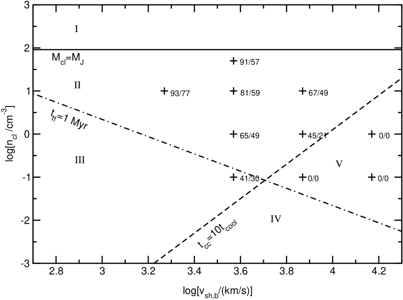
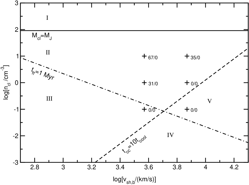
(A similar condition is given in Mellema, Kurk, & Röttgering (2002), Eq. 1.) In the context of shocks driven by jets from AGN, this illustrates that cooling can dominate over much of the parameter space of interest. The dashed line in Figure 3 separates the cooling-dominated regions from the non-cooling for a fixed cloud radius of $R_{cl}=100$ pc and density ratio $\chi=10^{3}$.

We arrive at another constraint by considering the free-fall timescale of the radiatively cooled gas, $\tau_{ff}$, which represents the shortest possible timescale on which stars can form within the cold gas. It also represents a typical spread over which star formation shall occur. As the first massive stars form, they provide an extra heating source in the cloud that will likely shut off any further star formation (Lin & Murray, 2000; Dong, Lin, & Murray, 2003). If we take 1 Myr as a typical star-formation timescale, then any gas with a longer free-fall timescale is unlikely to form stars efficiently. Thus we define $t_{ff}\leq 1$ Myr as our criterion for efficient star-formation. We can estimate the free-fall timescale $t_{ff}=(3\pi/32G\rho)^{1/2}$ by assuming that the cold cloud gas will eventually reach pressure equilibrium with the post-shock background. With this assumption, the final density of the cloud material is

$$\rho_{cl,f}\approx\frac{\mu m_{H}P_{b,ps}}{k_{B}T_{f}}~{}.$$ (20)

Using the shock-jump condition $P_{b,ps}\approx\rho_{b,i}v_{sh,b}^{2}=(\rho_{cl}v_{sh,b}^{2})/\chi$, we can write our star-formation criterion as

$$\left(\frac{t_{ff}}{\mathrm{Myr}}\right)\leq 1.5\left(\frac{\chi}{10^{3}}\right)^{1/2}\left(\frac{n_{cl}}{\mathrm{cm}^{-3}}\right)^{-1/2}\left(\frac{v_{sh,b}}{10^{3}\mathrm{km/s}}\right)^{-1}\left(\frac{T_{f}}{100\mathrm{K}}\right)^{1/2}~{}.$$ (21)

The dot-dashed line in Figure 3 shows this star-formation cut-off for specific values of $R_{cl}=100$ pc, $\chi=10^{3}$, $T_{f}=100$ K, and $t_{ff}=1$ Myr.

Two additional constraints come from the requirements that the cloud not be Jean’s unstable initially and that the shock velocity necessarily exceed the sound speed in the background gas. The first requirement gives us a constraint relation between the radius, temperature, and density of the cloud

$$\left(\frac{n_{cl}}{\mathrm{cm}^{-3}}\right)<91\left(\frac{R_{cl}}{100\mathrm{pc}}\right)^{-2}\left(\frac{T_{cl}}{10^{4}\mathrm{K}}\right)~{}.$$ (22)

The horizontal solid line in Figure 3 shows this stability limit for $R_{cl}=100$ pc and $T_{cl}=10^{4}$ K. The second requirement can be written as a relation between the velocity of the shock and the temperature of the cloud

$$\left(\frac{v_{sh,b}}{10^{3}\mathrm{km/s}}\right)>3.7\times 10^{2}\left(\frac{\chi}{10^{3}}\right)^{1/2}\left(\frac{T_{cl}}{10^{4}\mathrm{K}}\right)^{1/2}~{}.$$ (23)

This constraint is easily met by all of the parameters considered in this study and is not shown in Figure 3 (it would be a vertical line just off the left edge of the figure).

Thus we can divide our parameter space into five regions as shown in Figure 3. Region I (gravitationally unstable) is not of interest in this study. In regions IV and V cooling is expected to be negligible, so these are not of much interest either. Although cooling will be important in region III, the star-formation timescale is too long for the process to be very efficient. This leaves us with region II as the sector of primary interest in this study of shock-induced star formation. However, we also examine models in region V in order to confirm our above estimates of the location of the boundary between regions. The particular parameter pairs chosen for numerical study (marked with crosses in Figure 3) are discussed below.

4 Results

Table 1 summarizes the runs using the equilibrium cooling-curve model with solar metallicities. We choose ten combinations of $n_{cl}$ and $v_{sh,b}$ in order to explore the parameter space of interest indicated in Figure 3. The Mach number, $\mathcal{M}$, corresponding to each value of $v_{sh,b}$ is also listed. Finally, Table 1 also includes the shock-passage ($t_{sp}$), cloud-compression ($t_{cc}$), and cooling ($t_{cool}$) timescales for each run. Notice that the shock-passage and cloud-compression timescales vary by less than an order of magnitude, whereas the cooling timescale varies by almost 5 orders of magnitude among the models considered. This again arises from the very strong dependence of $t_{cool}$ on $v_{sh,b}$ and $n_{cl}$.

Table 2 summarizes the runs using the non-equilibrium primordial chemistry model. We choose a subset of six parameter combinations from those considered with the equilibrium cooling-curve model. Table 2 also includes the shock-passage ($t_{sp}$) and cloud-compression ($t_{cc}$) timescales for each run.

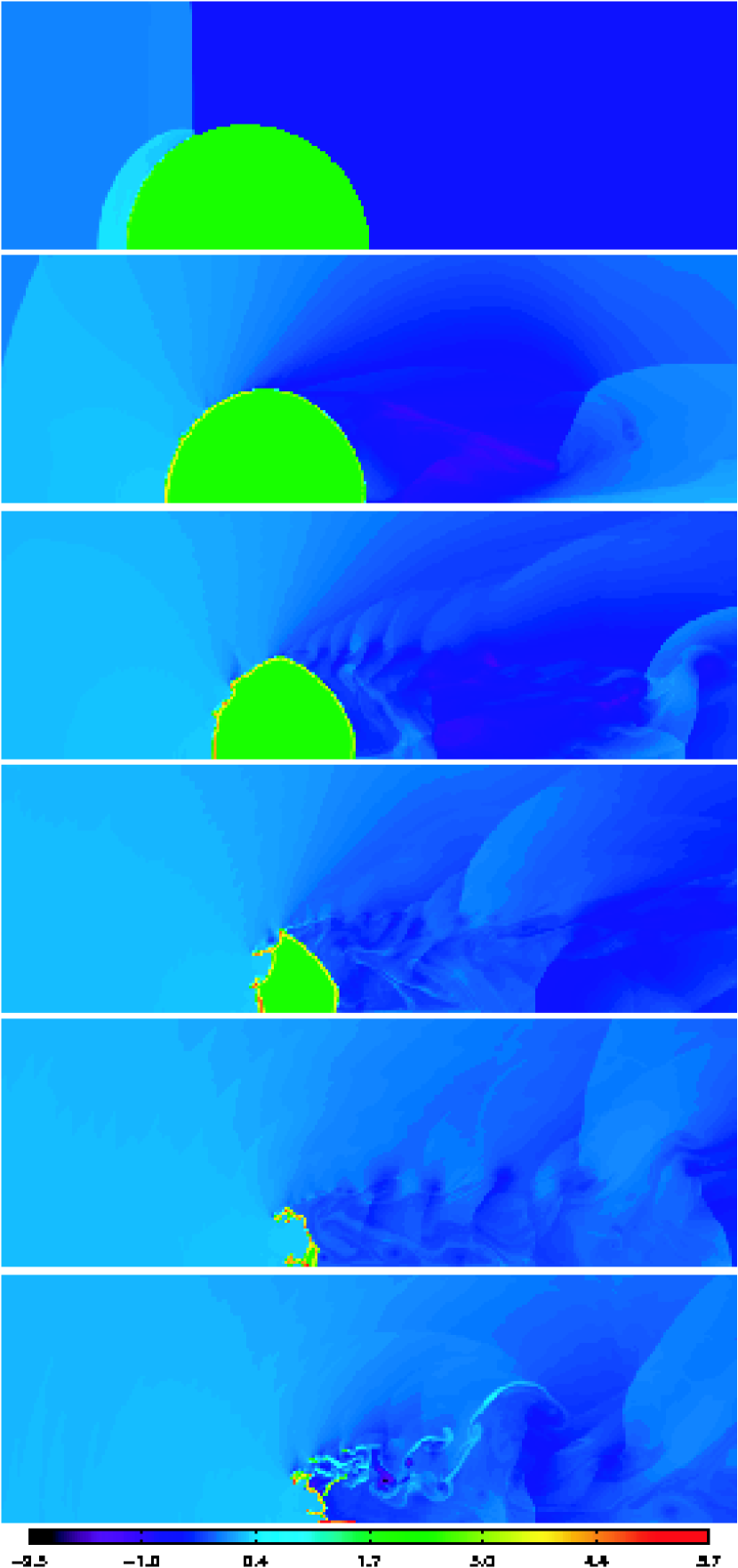
Figure 4 illustrates a sequence of density contour plots taken from the simulation of model E3. The parameters for this model were intentionally chosen to match those of run A in Mellema, Kurk, & Röttgering (2002). As expected, our results match theirs quite well. The strong cooling behind the compression shock in the cloud causes a very dense shell to form. The density of this shell continues to increase as it follows the compression shock into the center of the cloud. Hydrodynamic and radiative instabilities cause the cold shell to fragment as it progresses toward the center of the cloud. Similar results are seen in all of our cooling-dominated runs. As highlighted in Mellema, Kurk, & Röttgering (2002), the fragmentation is a unique result of hydrodynamic simulations of shock-cloud interactions in the cooling-dominated regime and is not observed in simulations that ignore radiative cooling (Klein, McKee, & Colella, 1994). In our simulations, the final densities of the fragments are often 3-4 orders of magnitude higher than the initial cloud density. However, as mentioned above, these final densities are generally limited by numerical resolution and are likely to underestimate the true final densities in these fragments. We are also unable to clearly resolve any interactions among either the main colliding shocks or the cold dense filaments of gas at late times.

4.1 Cooling Efficiency

We attempt to quantify the efficiency of the cooling processes in each of the runs presented. In order to accomplish this, we track the gas inside the cloud using a tracer fluid which is passively advected in the same manner as the density. Throughout each run the tracer distribution reflects the distribution of original cloud material. More importantly, it allows us to quantify how much of the initial cloud material cools below certain cutoff temperatures. Table 3 gives the percentages of cloud material that cool below $T=1000$ K and $T=100$ K for the equilibrium cooling curve models. The thermally unstable regime of cooling ends between $100$ and $1000$ K, so the fraction of gas with $T<1000$ K indicates the relative importance of cooling to the cloud evolution. Extensive star formation is unlikely, however, unless the gas is able to cool to $T<100$ K. The ability of the gas to reach such low temperatures in our equilibrium cooling curve models is, however, affected by numerical resolution and the neglection of self-gravity, both of which affect the peak density, and hence the cooling efficiency of the gas. Therefore, the percentage of gas that cools to below 1000 K gives a strong upper limit to the percentage that might form stars, while, when well resolved, the amount that cools to below 100 K gives a more accurate measure. These results are also represented graphically in Figure 3. We see that the equilibrium cooling curve results agree quite well with the expected transition from the non-cooling to the cooling-dominated regime, shown by the dashed line.

We also note from the results that the cooling process is generally extremely efficient throughout the cloud. In the most extreme case considered using the equilibrium cooling-curve (model E2), 77% of the gas in the cloud or $7.7\times 10^{5}M_{\odot}$ cools below 100 K. Large fractions of cool gas were seen in all of the other models within region II. The smallest value (21%) occurs near the boundary between regions II and V, while a more typical average seen for the models is approximately 50%. The primary exception is in model E6b, in which three clouds were modeled (see below).

Table 4 reports these same percentages for the non-equilibrium chemistry models. As expected, none of these models cool below 100 K (see §3.1.2), although many of them show substantial cooling below 1000 K. Cooling is also less efficient in these models than with the equilibrium cooling-curve. In the non-equilibrium chemistry models, cooling below $10^{4}$ K is due solely to H₂ emission. While H₂ is an efficient coolant, the small fractions formed via gas-phase reactions (Table 4) are insufficient to lead to cooling as extensive as that due to metals, which dominate the equilibrium cooling curve models. Based upon our numerical results, it appears the cooling timescales for the non-equilibrium chemistry models are roughly a factor of 10 longer than for the equilibrium cooling curve models using the same parameters. The decreased cooling efficiency leads to a shift in the boundary between regions II and V towards higher densities and lower shock speeds, as can be seen in Figure 5. Nevertheless, large fractions of the gas contained within the clouds still cool to below 1000 K. Given higher grid resolution, self-gravity, and an extended chemical network including metals, each of which would be expected to enhance the cloud densities and therefore the H₂ formation and cooling, a substantial fraction of gas might also be expected to cool below 100 K. The results indicate, therefore, that star formation may be extremely efficient in shocked clouds for which the cooling timescales are sufficiently short.

4.1.1 Self-Gravity

The initial free-fall timescales for our models vary from $7.3\times 10^{6}$ Myr for $n_{cl}=50$ cm^-3 (run E1) to $1.6\times 10^{8}$ Myr for $n_{cl}=0.1$ cm^-3 (runs E8-E10). As explained above, our parameters were deliberately chosen such that the clouds would not be gravitationally unstable initially and that the free-fall timescale would be longer than the dynamical timescale (taken as the cloud compression time $t_{cc}$). Nevertheless, as we have seen, the density of the gas increases substantially in the radiative shell behind the compression shock. Therefore the local free-fall time of this compressed gas will be much shorter than its initial value. This, of course, is the basis of the shock-induced star-formation model.

For a fairly typical density increase of $10^{4}$, the local free-fall timescale will decrease by $10^{2}$. In the coldest gas, the temperature decreases by more than two orders of magnitude from its original value, and so the cold, dense regions have Jeans masses reduced by five orders of magnitude relative to the original cloud. Thus, for the higher density runs (E1-E4), the self-gravity of the gas becomes dynamically important in the dense fragments behind the compression shock. Although the Cosmos code used in this study includes an option for solving self-gravity, most of our runs did not utilize it. In the two-dimensional limit considered in the current study, we would be solving the gravity of an infinite cylindrical cloud, which is notably different than the self-gravity of a spheroidal cloud. Nevertheless, we did conduct one run (E1b) with the self-gravity option turned on. The enhanced compression due to self-gravity did allow the gas to cool more efficiently than the corresponding run without self-gravity (E1a). As a result, 69% of the gas in model E1b cooled to below 100 K, as compared to 57% in model E1a.

4.1.2 Multiple Clouds

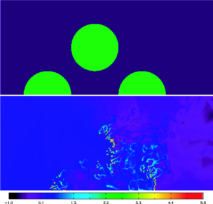
For most of this study we consider the interaction of a planar shock with a single cloud. However, our general notion of jet-induced star formation envisions the interaction of such a shock with a system of clouds within an inhomogeneous background. To highlight the possible effects of the interaction of multiple clouds, we have considered one run with a system of four clouds: two aligned perpendicular to the shock front, and two aligned parallel to it. This set up allows us to achieve higher spatial resolution by imposing symmetry boundary conditions and computing only half of the problem. Each individual cloud has the same parameters as the single cloud in model E6a ($R_{cl}=100$ pc, $T_{cl}=10^{4}$ K, and $n_{cl}=1$ cm^-3). The initial cloud configuration is shown in the top of Figure 6. The size of the computational grid and the number of zones are scaled equally to maintain the same $0.5\times 0.5$ pc per zone resolution as our other runs.

The interaction of these clouds results in less efficient cooling throughout all of the clouds, but particularly for those in the downwind direction. The leading cloud, in fact, cools almost identically to the isolated cloud case. The discrepancy in the amount of gas found below our 100 K threshold (9% for the front cloud in run E6b versus 21% for the isolated cloud in run E6a) disappears if we change the lower threshold to 200 K. The amount of gas below that threshold is 28% for both models. This indicates that there is a significant amount of gas near 100 K in both models, but in the multi-cloud model most of it is just above this threshold.

The reduced amount of cold gas in the downwind clouds is likely due to a combination of effects. First, geometric screening of the primary shock results in less symmetric, and generally less efficient, compression for the downwind clouds. The close proximity of the clouds in this simulation also subjects them to multiple reflected shocks from their neighbors which can reheat previously cooled gas. This may be enhanced in the present work by the symmetry imposed by the two-dimensional geometry. In three dimensions, these reflected shocks would presumably be less focused. Finally, consistent with Poludnenko, Frank, & Blackman (2002), we find that the channel between the clouds acts as a de Lavalle nozel and accelerates the background gas. Since both the Rayleigh-Taylor and Kelvin-Helmholtz instabilities scale as the inverse of the background velocity, this acceleration reduces the destruction time for the downwind clouds. This effect may be reduced in three dimensions.

The results of this multi-cloud run suggest that the efficiencies we quote for our single cloud runs should generally be viewed as applicable to relatively isolated clouds. We note, however, that although reduced by a factor of a few relative to the single-cloud models, the fraction of cold gas is still significant in the model with multiple clouds. In future work we plan to present a more detailed study of the interactions of shocks with systems of radiating clouds.

4.2 H₂ Formation

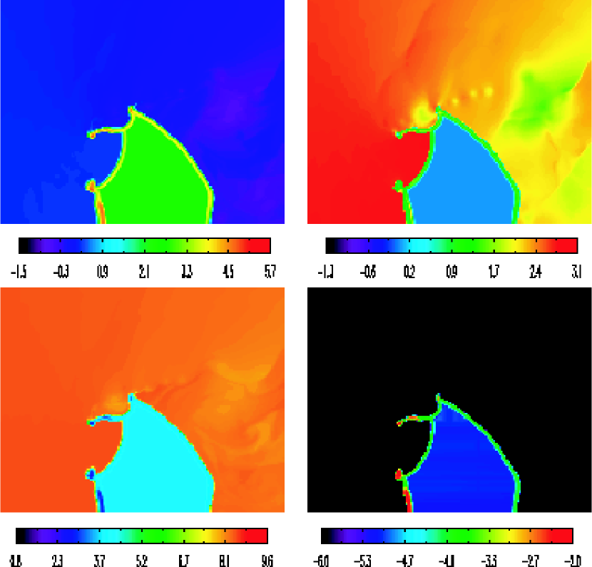
Table 4 also lists the local peak mass fraction of H₂ [max($\rho_{H_{2}}/\rho$)] and the total H₂ mass fraction ($M_{H_{2}}/M_{cl}$) for the non-equilibrium chemistry models, where $M_{H_{2}}$ is the total mass of H₂ at the end of each run ($t=1.25t_{cc}$) and $M_{cl}$ is the initial cloud mass. The observed H₂ mass fractions are consistent with the results of Anninos et al. (1997). Figure 7 illustrates how the H₂ distribution, temperature, density, and pressure trace each other for model C1a.

4.2.1 Chemistry Parameters

Along with the six combinations of $n_{cl}$ and $v_{sh,b}$ studied with the non-equilibrium chemistry model, we also explore the dependence of our results on our treatments of photoionization and photodissociation. Model C1a is our base model, comparable to the equilibrium-cooling model E3. Models C1a and C2-C6 include photoionization, photodissociation, and integrated optical depth calculations. Model C1b ignores photoionization and photodissociation. In the absence of these processes, there is also no need to calculate any optical depths. This run results in a slightly higher percentage of gas cooling below 1000 K, relative to model C1a, due to a higher mass fraction of H₂. Model C1c includes photoionization and photodissociation but does not include optical depth calculations. The omission of self-shielding results in a dramatic reduction in the amount of gas which is able to cool below 1000 K and in the amount of H₂ that forms, illustrating the importance of self-shielding. Model C1d increases the strength of the external photoionization field by a factor of 10. This produces a slight increase in the percentage of gas able to cool below 1000 K, due to the increased ionization fraction, which, in turn, enhances the formation of H₂ via H^-. Model C1e increases the H₂ photoreactive destruction rate coefficient ($k27$) by an order of magnitude. This results in a reduction of about 14% in the amount of gas cooling below 1000 K and a dramatic reduction in the final quantity of H₂.

5 Implications for Cloud and Jet Evolution

Our numerical studies have concentrated primarily on following the evolution of a single dense cloud being overrun by a planar shock traveling through a low density background. This picture is intended to represent what is happening on a relatively small scale ($\sim 100$ pc) within a much larger region of interaction ($\gtrsim 1$ kpc) between a jet-induced shock and an inhomogeneous medium. We now generalize our results to predict some properties of jet-induced star-forming regions.

5.1 Star Formation Rates

We first wish to consider the star-formation rate for this process. To arrive at this, we need to estimate the rate at which the mass of gas in dense clumps is swept over by the shock. This is given by

$$\dot{M}_{cl}=f_{cl}\rho_{cl}v_{sh}A~{},$$ (24)

where $f_{cl}$ is the volume filling factor of the clumps and $A$ is the surface area of the shock front. The star-formation rate is the mass rate multiplied by the star-formation efficiency. Here it will help to consider a specific object, so we take Minkowski’s Object. From our simulations in §2.1, we estimate the shock speed inside the cloud to be $\approx 3\times 10^{8}$ cm s^-1. From van Breugel et al. (1985) we take $A\approx 20$ kpc², where we assume, for simplicity, that the cross-sectional area is constant. Then, for a single dense phase of $\rho_{cl}\approx 10^{-23}$ g cm^-3, we can match the observed star-formation rate of $\sim 0.3M_{\odot}$ yr^-1 by assuming a volume filling factor of $f_{cl}\approx 0.03$ and a star-formation efficiency of 0.1%.

5.2 Acceleration of Clouds and Mass Loading

We have already estimated the acceleration timescale of these clouds in §2.2. From this we can estimate their velocities as a function of time. In terms of the typical parameters considered in this study, we get

$$\left(\frac{v_{cl}}{\mathrm{km/s}}\right)\lesssim 20\left(\frac{\chi}{10^{3}}\right)^{-1}\left(\frac{R_{cl}}{100\mathrm{pc}}\right)^{-1}\left(\frac{v_{sh,b}}{10^{3}\mathrm{km/s}}\right)^{2}\left(\frac{t}{\mathrm{Myr}}\right)~{}.$$ (25)

This value seems to overestimate the cloud velocity by a factor of a few based upon our numerical results. However, this is reasonable since the estimate assumes a constant cross-sectional area for the cloud. As we have seen, the cross-sectional area can be reduced significantly during compression. The final conclusion is that, for the parameter space studied, these clouds accelerate very slowly. We note that, for Minkowski’s Object, this is in good agreement with observations, which show very little evidence for velocity gradients in the ionized gas downstream from the jet-cloud collision region.

Along with the potential of becoming starburst regions, the nearly stationary cloud fragments may also become significant sources of mass loading for the post-shock flow (Hartquist & Dyson, 1988). Mass loading is the feeding of material into the flow and could have a significant impact on its properties, including possibly causing it to transition to the transonic regime. However, it is difficult to estimate the significance of mass loading from our simulations. Over the evolution time of our models ($1.25t_{cc}$), very little mass is lost from the clouds (typically $\lesssim$ 1%). This amount would certainly increase if longer evolution times were considered, but as we pointed out in §3 we can not reliably follow the evolution of these clouds beyond the current limits since our numerical resolution prevents further compression of the clouds. The question of mass loading is one we will return to in future studies.

6 Conclusions

We have performed two-dimensional simulations of the evolution of radiatively cooling clouds subjected to strong shocks, as might arise from galactic jets. The results of the models are summarized in Figures 3 and 5, which show the locations of the models in cloud density-shock velocity parameter space. Figure 3 presents the results for models which include equilibrium cooling with solar abundances, while Figure 5 shows the results for primordial clouds, which include non-equilibrium chemistry in which cooling at low temperatures is dominated by H₂ emission. The numbers by each model indicate the percentages of the original gas that cools to below either 1000 K or 100 K. As can be seen from the figures, large fractions ($\gtrsim 1/3$) of the clouds are able to cool below 1000 K. Most of this cold gas ends up in very dense filaments, which have long dynamical lifetimes. The final densities of these filaments are high enough in many cases that they are gravitationally unstable. The subsequent gravitational collapse of these regions will likely result in a burst of star formation. Our numerical results are consistent with previous work (e.g. Mellema, Kurk, & Röttgering, 2002) and have extended it by including new physics (chemistry and self-gravity) and exploring more of the parameter space of interest.

We applied our results to the specific example of Minkowski’s Object. A number of important conclusions can be drawn. First, its peculiar morphology - bright star forming region orthogonal to the jet, and fainter filamentary features downstream from there - can be easily reproduced by our simulations (Fig 1). Second, the modest amount star formation required - $0.3M_{\odot}$ yr^-1 for the entire object, is also easily achieved for the plausible parameter space explored by our simulations. Third, and most interestingly, we conclude that the star formation in Minkowski’s Object could be induced by a moderate velocity jet ($9\times 10^{4}$ km s^-1) interacting with a collection of slightly overdense ($\sim 10$ cm^-3), warm ($10^{4}$ K) clouds, i.e. it is NOT necessary to assume that this was an accidental collision between a jet and a preexisting gas-rich galaxy. This also suggests that the neutral hydrogen associated with Minkowski’s Object ($3\times 10^{8}M_{\odot}$; W. van Breugel & J. van Gorkom 2003, private communication) may have cooled from the warm gas phase as a result of the radiative cooling triggered by the radio jet. An update on the observations of Minkowski’s Object will be presented in a forthcoming paper (S. D. Croft et al., in preparation).

Our results show that jets can drive radiative shocks in overdense regions in the intergalactic medium, resulting in star formation far away from the galaxies in which the jets originate. This could be an important factor in understanding the feedback of AGN on their environment. Our simulations may also be applied to radiative shocks and resulting star formation triggered by other mechanisms, such as in the wake of supernova blast waves (Preibisch et al., 2002), collisions of interstellar or intergalactic clouds (Smith, 1980), and ram pressure on gas-rich galaxies that fall into galaxy cluster atmospheres (e.g. Gavazzi et al., 2001).

Our models can be used to infer the importance of shock-induced star formation in other regimes by simply adjusting the criteria used to develop Figure 3. Our models have confirmed the reality of the division between regions II and V (cooling and non-cooling) derived using approximate analytical methods, while the other region boundaries are set by physical limits for the clouds. In future work, we shall extend our numerical simulations into regimes appropriate for other possible shock-cloud interaction scenarios.

Table 1: Equilibrium Cooling Curve Models

	$n_{cl}$	$v_{sh,b}$		$t_{sp}$	$t_{cc}$	$t_{cool}$
Model	(cm-3)	(103 km s-1)	$\mathcal{M}$	(yr)	(yr)	(yr)	Notes
E1a	50	3.7	10	$5.3\times 10^{4}$	$8.5\times 10^{5}$	$3.9\times 10^{1}$
E1b	50	3.7	10	$5.3\times 10^{4}$	$8.5\times 10^{5}$	$3.9\times 10^{1}$	self gravity
E2	10	1.9	5	$1.1\times 10^{5}$	$1.7\times 10^{6}$	$2.4\times 10^{1}$
E3	10	3.7	10	$5.3\times 10^{4}$	$8.5\times 10^{5}$	$1.9\times 10^{2}$	(C1a)
E4	10	7.4	20	$2.7\times 10^{4}$	$4.3\times 10^{5}$	$1.6\times 10^{3}$	(C2)
E5	1	3.7	10	$5.3\times 10^{4}$	$8.5\times 10^{5}$	$1.9\times 10^{3}$	(C3)
E6a	1	7.4	20	$2.7\times 10^{4}$	$4.3\times 10^{5}$	$1.6\times 10^{4}$	(C4)
E6b	1	7.4	20	$2.7\times 10^{4}$	$4.3\times 10^{5}$	$1.6\times 10^{4}$	multi-cloud
E7	1	14.9	40	$1.3\times 10^{4}$	$2.1\times 10^{5}$	$1.2\times 10^{5}$
E8	0.1	3.7	10	$5.3\times 10^{4}$	$8.5\times 10^{5}$	$1.9\times 10^{4}$	(C5)
E9	0.1	7.4	20	$2.7\times 10^{4}$	$4.3\times 10^{5}$	$1.6\times 10^{5}$	(C6)
E10	0.1	14.9	40	$1.3\times 10^{4}$	$2.1\times 10^{5}$	$1.2\times 10^{6}$

Table 2: Non-equilibrium Chemistry Models

	$n_{cl}$	$v_{sh,b}$		$t_{sp}$	$t_{cc}$
Model	(cm-3)	(km s-1)	$\mathcal{M}$	(yr)	(yr)	Notes
C1a	10	3.7	10	$5.3\times 10^{4}$	$8.5\times 10^{5}$	(E3)
C1b	10	3.7	10	$5.3\times 10^{4}$	$8.5\times 10^{5}$	No photo-ionization or photo-dissociation
C1c	10	3.7	10	$5.3\times 10^{4}$	$8.5\times 10^{5}$	No optical depth calculations
C1d	10	3.7	10	$5.3\times 10^{4}$	$8.5\times 10^{5}$	Photoionizing field 10 times stronger
C1e	10	3.7	10	$5.3\times 10^{4}$	$8.5\times 10^{5}$	Photodissociation rate 10 times higher
C2	10	7.4	20	$2.7\times 10^{4}$	$4.3\times 10^{5}$	(E4)
C3	1	3.7	10	$5.3\times 10^{4}$	$8.5\times 10^{5}$	(E5)
C4	1	7.4	20	$2.7\times 10^{4}$	$4.3\times 10^{5}$	(E6a)
C5	0.1	3.7	10	$5.3\times 10^{4}$	$8.5\times 10^{5}$	(E8)
C6	0.1	7.4	20	$2.7\times 10^{4}$	$4.3\times 10^{5}$	(E9)

Table 3: Equilibrium Cooling Curve Results

	Gas with
	$T_{f}<1000$ K	$T_{f}<100$ K
Model	(% of $M_{cl}$)	(% of $M_{cl}$)
E1a	91	57
E1b	92	69
E2	93	77
E3	81	59
E4	67	49
E5	65	49
E6a	45	21
E6b	46,26,21	9,16,17
E7	0	0
E8	41	30
E9	0	0
E10	0	0

Table 4: Non-Equilibrium Chemistry Results

	Gas with			H2 Mass Fraction
	$T_{f}<1000$ K	$T_{f}<100$ K		Peak	Total
Model	(% of $M_{cl}$)	(% of $M_{cl}$)		($\rho_{H_{2}}/\rho$)	($M_{H_{2}}/M_{cl}$)
C1a	67	0		$1.3\times 10^{-2}$	$1.3\times 10^{-5}$
C1b	72	0		$4.0\times 10^{-2}$	$3.9\times 10^{-5}$
C1c	13	0		$6.3\times 10^{-4}$	$1.0\times 10^{-6}$
C1d	69	0		$3.2\times 10^{-2}$	$2.5\times 10^{-5}$
C1e	53	0		$1.0\times 10^{-2}$	$3.9\times 10^{-6}$
C2	35	0		$1.0\times 10^{-2}$	$8.3\times 10^{-6}$
C3	31	0		$5.0\times 10^{-3}$	$6.9\times 10^{-7}$
C4	0	0		$4.0\times 10^{-4}$	$4.6\times 10^{-7}$
C5	0	0		$1.0\times 10^{-4}$	$7.6\times 10^{-8}$
C6	0	0		$1.3\times 10^{-4}$	$3.9\times 10^{-8}$

Figure 1: Contour plot of the logarithm of gas density for a simulation of a jet colliding with the long axis of an elliptical cloud at simulation times $t=0.1$, 0.8, 1.4, and 2.1 Myr. The unit for the density scale in this plot is $1.7\times 10^{-28}$ g cm^-3, corresponding to an initial cloud mass of $\approx 10^{9}M_{\odot}$.

Figure 2: Comparison of an intermediate density distribution plot from the numerical simulation in Figure 1 with a similarly scaled observation of Minkowski’s Object. There are clear similarities between the distribution of the post-shock gas within the simulated cloud (colored red) and the regions of active star formation within Minkowski’s Object.

Figure 3: General cloud number density ($n_{c}l$)-shock velocity ($v_{sh,b}$) parameter space considered. The solid line demarks the density above which the cloud is initially gravitationally unstable (region I). The dashed line divides the cooling dominated regions (II & III) on the left from the non-cooling regions (IV & V) on the right. The dot-dashed line is an estimate of the star-formation cut-off. Hence clouds in region III will likely form far fewer stars than those found in region II. The particular parameter pairs explored with the equilibrium cooling curve model are indicated with crosses. The two numbers next to each cross give the amount of cloud gas that ends the simulation below $T=1000$ and 100 K, respectively, as a percent of the initial cloud mass.

Figure 4: Contour plots of the logarithm of gas density for model E3 at times $t=0.05$, 0.25, 0.5, 0.75, 1.0, and 1.25 $t_{cc}$. The units for the density scale in this plot are $6.7\times 10^{-26}$ g cm^-3, corresponding to an initial cloud density of $1.7\times 10^{-23}$ g cm^-3. Each frame shows the full computational grid, with physical dimensions of $600\times 200$ pc.

Figure 5: Same as Figure 3 except applies to the non-equilibrium chemistry model.

Figure 6: Contour plot of the logarithm of gas density for model E6b at times $t=0$ and $1.25t_{cc}$. The units for the density scale in this plot are $6.7\times 10^{-27}$ g cm^-3, corresponding to an initial cloud density of $1.7\times 10^{-24}$ g cm^-3. Each frame shows the full computational grid, with physical dimensions of $900\times 400$ pc.

Figure 7: Contour plot of the logarithm of gas density (upper left), gas pressure (upper right), temperature (lower left), and H₂ mass fraction (lower right) for model C1a at time $t=0.75t_{cc}$. The corresponding units are: $1.7\times 10^{-23}$ g cm^-3 for density and $8.9\times 10^{-12}$ g cm^-1 s^-2 for pressure. The temperature unit is Kelvin. The H₂ mass fraction measures $\rho_{H_{2}}/\rho$. The plots only show a small portion of the overall computational domain.

References

- Anninos & Fragile (2003) Anninos, P., & Fragile, P. C. 2003, ApJS, 144, 243
- Anninos, Fragile & Murray (2003) Anninos, P., Fragile, P. C., & Murray, S. D. 2003, ApJS, 147, 177
- Anninos et al. (1997) Anninos, P., Zhang, Y., Abel, T., & Norman, M. L. 1997, New Astronomy, 2, 209
- Bechtold et al. (1987) Bechtold, J., Weymann, R. J., Lin, Z., & Malkan, M. A. 1987, ApJ, 315, 180
- Begelman & Cioffi (1989) Begelman, M. C. & Cioffi, D. F. 1989, ApJ, 345, L21
- Bicknell (1984) Bicknell, G. V. 1984, ApJ, 286, 68
- Bicknell et al. (2000) Bicknell, G. V., Sutherland, R. S., van Breugel, W. J. M., Dopita, M. A., Dey, A., & Miley, G. K. 2000, ApJ, 540, 678
- Blanco et al. (1975) Blanco, V. M., Graham, H. A., Lasker, B. M., & Osmer, P. S. 1975, ApJ, 198, L63
- Chambers, Miley, & van Breugel (1987) Chambers, K. C., Miley, G. K., & van Breugel, W. 1987, Nature, 329, 604
- Chandrasekhar (1961) Chandrasekhar, S. 1961, Hydrodynamic and Hydromagnetic Stability (New York: Dover)
- Dalgarno & McCray (1972) Dalgarno, A., & McCray, R. A. 1972, ARA&A, 10, 375
- Dey et al. (1997) Dey, A., van Breugel, W., Vacca, W. D., & Antonucci, R. 1997, ApJ, 490, 698
- De Young (1989) De Young, D. S. 1989, ApJ, 342, L59
- Dong, Lin, & Murray (2003) Dong, S., Lin, D. N. C., & Murray, S. D. 2003, ApJ, in press
- Fanaroff & Riley (1974) Fanaroff, B. L. & Riley, J. M. 1974, MNRAS, 167, 31P
- Ferland, Fabian, & Johnstone (2002) Ferland, G. J., Fabian, A. C., & Johnstone, R. M. 2002, MNRAS, 333, 876
- Field (1965) Field, G. B. 1965, ApJ, 142, 531
- Gavazzi et al. (2001) Gavazzi, G., Boselli, A., Mayer, L., Iglesias-Paramo, J., Vílchez, J. M., & Carrasco, L. 2001, ApJ, 563, L23
- Gregori et al. (1999) Gregori, G., Miniati, F., Ryu, D., & Jones, T. W. 1999, ApJ, 527, L113
- Hartquist & Dyson (1988) Hartquist, T. W. & Dyson, J. E. 1988, Ap&SS, 144, 615
- Hollenbach, Werner, & Salpeter (1971) Hollenbach, D. J., Werner, M. W., & Salpeter, E. E. 1971, ApJ, 163, 165
- Kahn (1976) Kahn, F. D. 1976, A&A, 50, 145
- Klein, McKee, & Colella (1994) Klein, R. I., McKee, C. F., & Colella, P. 1994, ApJ, 420, 213
- Laing & Bridle (2002) Laing, R. A. & Bridle, A. H. 2002, MNRAS, 336, 1161
- Lepp & Shull (1983) Lepp, S. & Shull, J. M. 1983, ApJ, 270, 578
- Lin & Murray (2000) Lin, D. N. C. & Murray, S. D. 2000, ApJ, 540, 170
- McCarthy et al. (1987) McCarthy, P. J., van Breugel, W. J. M., Spinrad, H., & Djorgovski, S. 1987, ApJ, 321, L29
- McNamara (2002) McNamara, B. R. 2002, New Astronomy Review, 46, 141
- Mellema, Kurk, & Röttgering (2002) Mellema, G., Kurk, J. D., Röttgering, H. J. A. 2002, A&A, 395, L13
- Mould et al. (2000) Mould, J. R. et al. 2000, ApJ, 536, 266
- Murray & Lin (1989) Murray, S. D. & Lin, D. N. C. 1989, ApJ, 339, 933 (see also Erratum, 1989, ApJ, 344, 1052)
- Osterbrock (1989) Osterbrock, D. E. 1989, Astrophysics of Gaseous Nebulae and Active Galactic Nuclei (Mill Valley: University Science Books)
- Poludnenko, Frank, & Blackman (2002) Poludnenko, A. Y., Frank, A., & Blackman, E. G. 2002, ApJ, 576, 832
- Preibisch et al. (2002) Preibisch, T., Brown, A. G. A., Bridges, T., Guenther, E., & Zinnecker, H. 2002, ApJ, 124, 404
- Rees (1989) Rees, M. J. 1989, MNRAS, 239, 1P
- Rejkuba et al. (2002) Rejkuba, M., Minniti, D., Courbin, F., & Silva, D. R. 2002, ApJ, 564, 688
- Reuland et al. (2003) Reuland, M. et al. 2003, ApJ, 592, 755
- Sgro (1975) Sgro, A. G. 1975, ApJ, 197, 621
- Smith (1980) Smith, J. 1980, ApJ, 238, 842
- Spaans & Neufeld (1997) Spaans, M. & Neufeld, D. A. 1997, ApJ, 484, 785
- van Breugel et al. (1985) van Breugel, W., Filippenko, A. V., Heckman, T., & Miley, G. 1985, ApJ, 293, 83
- van Breugel et al. (1999) van Breugel, W., Stanford, A., Dey, A., Miley, G., Stern, D., Spinrad, H., Graham, J., & McCarthy, P. 1999, in The Most Distant Radio Galaxies, ed. H. J. A. R ttgering, P. N. Best, & M. D. Lehnert (Amsterdam: Royal Netherlands Academy of Arts and Sciences), 49