Time-sequenced Multi-Radio-Frequency Observations of Cygnus X-3 in Flare

Abstract

Multifrequency observations from the VLA, VLBA and OVRO Millimeter Array of a major radio outburst of Cygnus X-3 in 2001 September are presented, measuring the evolution of the spectrum of the source over three decades in frequency, over a period of six days. Following the peak of the flare, as the intensity declines the high-frequency spectrum at frequency $\nu$ steepens from $\nu^{-0.4}$ to $\nu^{-0.6}$, after which the spectral index remains at this latter terminal value; a trend previously observed but hitherto not satisfactorily explained. VLBA observations, for the first time, track over several days the expansion of a sequence of knots whose initial diameters are $\sim 8$ milliarcseconds. The light-crossing time within these plasmons is of the same order as the time-scale over which the spectrum is observed to evolve. We contend that properly accounting for light-travel time effects in and between plasmons which are initially optically thick, but which after expansion become optically thin, explains the key features of the spectral evolution, for example the observed timescale. Using the VLBA images, we have directly measured for the first time the proper motions of individual knots, analysis of which shows a two-sided jet whose axis is precessing. The best-fit jet speed is $\beta\sim 0.63$ and the precession period is $\sim 5$ days, significantly lower than fitted for a previous flare. Extrapolation of the positions of the knots measured by the VLBA back to zero-separation shows this to occur approximately 2.5 days after the detection of the rise in flux density of Cygnus X-3.

1 Introduction

Cygnus X-3 was first detected by Giacconi et al. (1967) using X-ray proportional counters during a 1966 rocket flight and rose to prominence with the detection of a giant radio flare in 1972 September (Gregory et al., 1972a). It is a high-mass X-ray binary system located in the Galactic plane at a distance of $\approx$10 kpc from the Earth (Predehl et al., 2000; Dickey, 1983). With Galactic co-ordinates $l=79.84$^∘, $b=0.69$^∘, it lies in or behind either the Perseus or the Outer Arm, depending on its exact distance from us. The nature of the compact object is still uncertain. The large interstellar extinction to the source precludes optical spectroscopy, making it difficult to obtain a reliable mass function and hindering identification of the companion star. However, infrared spectra show strong, broad helium emission lines, and a lack of strong hydrogen emission. Spectral analysis by van Kerkwijk et al. (1996) indicated that the companion is a Wolf-Rayet star of the WN7 subclass, although more recent observations by Koch-Miramond et al. (2002) suggested that the subclass may in fact be WN8. The orbital period, as inferred from X-ray and infrared flux modulations, is 4.8 hours (e.g. Parsignault et al., 1972). This source occasionally undergoes huge radio outbursts where the flux density can increase up to levels of $\sim 20$ Jy. Of order 50 outbursts with peak radio flux densities exceeding 1 Jy have been observed since the detection of the first such flare in 1972 September. During one of these radio outbursts, the hard X-ray emission was found to correlate strongly with the radio emission, although the soft X-ray emission was anticorrelated with radio flux density (McCollough et al., 1999). In quiescence, the soft-X-ray is found to be strongly correlated with the radio emission, and anticorrelated with the hard X-rays (Choudhury et al., 2002). This soft-X-ray—radio correlation disappears immediately before and during periods of radio flaring (Watanabe et al., 1994). During recent outbursts, jet-like structures have been observed at radio frequencies, although there has been some debate as to the morphology of the collimated emission. Two-sided jets from a flare in 2000 September were detected on arcsecond scales in a north-south orientation with the Very Large Array (VLA) (Martí et al., 2001), with an inferred jet speed $v=0.48c$. On milliarcsecond scales, a one-sided jet with the same orientation was imaged with the Very Long Baseline Array (VLBA) after a flare in 1997 February (Mioduszewski et al., 2001). In this case, the derived jet speed was significantly higher ($v\geq 0.81c$).

In this paper we analyse radio observations of the 2001 September outburst of Cygnus X-3 and describe some of the physical mechanisms responsible for the observed evolution of the source. In §2 we summarize the characteristics of previous radio flares of Cygnus X-3. In §3, §4 and §5, we present our observations from the VLA, Owens Valley Radio Observatory (OVRO) Millimeter Array, and the VLBA respectively, and in §6 we analyse the VLBA images and infer the speed, sidedness and precession parameters of the jet. We go on to discuss the spectral evolution and the underlying physical mechanisms for the low-frequency turnover in §7. We then derive constraints on the magnetic field strength, electron number density and energy density in the source in §8, and describe the physics behind the high-frequency spectral evolution in §9. In §10 the magnetic field strength and energy in the jet in this outburst of Cygnus X-3 are compared to derived parameters of radio galaxies such as Cygnus A and M 87.

2 Spectral characteristics

The temporal evolution of the radio spectrum of Cygnus X-3 was first studied during the outburst of 1972 September (Gregory et al., 1972a, and 20 papers following this). This outburst was observed between 0.4 GHz and 90 GHz, and observations were made during both the increase and the subsequent decrease of the radio flux density. This outburst of Cygnus X-3 exhibited approximately similar characteristics to several other major flares observed from this system: a short-lived exponential fading of the intensity (e.g. Aller & Dent, 1972; Hjellming et al., 1974; Marsh et al., 1974; Waltman et al., 1995) with $e$-folding times $\tau$ in the range $0.15<\tau<2.75$ days, followed by a power-law decay in intensity. With sufficient frequency coverage a two-phase spectral evolution is seen; an initial steepening of the spectrum, after which the spectral index $\alpha$ (which relates the intensity $S_{\nu}$ to the frequency $\nu$ as $S_{\nu}\propto\nu^{-\alpha}$) remains at a terminal value of $\sim 0.6-0.7$ (e.g. Gregory et al., 1972b; Aller & Dent, 1972; Hjellming & Balick, 1972; Seaquist et al., 1974; Geldzahler et al., 1983; Fender et al., 1997). In the dataset we present in this paper, we have observations over a wider frequency range than made previously, which more tightly constrain the observed evolution. However, our observations were not triggered early enough to observe the rise phase of the outburst, which precludes detailed modelling of the mechanism responsible for launching the jet, and comparison with previous models purporting to explain the rise phase of radio flares (e.g. Martí et al., 1992).

3 VLA observations and data reduction

The outburst of Cygnus X-3 was observed to begin when the radio flux density started to rise on 2001 September 14 (MJD $52167\pm 0.2$) (Trushkin et al., 2002), and was monitored regularly with the VLA from September 18 until ten days following the outburst, and then less frequently until the end of October. The VLA was in its most compact “D” configuration, so that the source was unresolved and, crucially, the VLA measured the integral of all emission regions associated with the outburst. The source was observed using snapshot observations of duration two to three minutes, sufficient to detect and perform photometry on the source.

Data were taken with the VLA using standard procedures, observing at eight different frequency bands (centred on 73.8 MHz, 327.5 MHz, 1.425 GHz, 4.86 GHz, 8.46 GHz, 14.94 GHz, 22.46 GHz, and 43.34 GHz). A summary of the observing dates and frequencies may be found in Table 1. All observations except for those at 73.8-MHz were made in two independent frequency bands (IF pairs). All IFs were of width 50 MHz except for the 327.5- and 73.8-MHz data, which had bandwidths of 3.125 and 1.563 MHz respectively. At 1.425 GHz, the two IFs (with frequencies of 1.465 and 1.385 GHz for the upper and lower sidebands respectively) were imaged separately, to gain an extra low-frequency point where the spectral shape was changing most rapidly. At all other frequencies, the data in the separate IFs were averaged together during imaging. Calibration and image processing were performed using NRAO’s Astronomical Image Processing System (AIPS). The primary calibrators used were 3C 48 and 3C 286, depending on which was above the horizon at the time of the observation. One of these was observed at each frequency in every observing run. The flux scale used was that derived at the VLA in 1999, as implemented in the 31Dec02 version of AIPS. Several different secondary calibrators were used, depending on the frequency of observation and on the other sources observed during the run. These were J 2007+4029, J 2015+3710, and J 1953+3537, at angular separations of 4.7$\arcdeg$, 5.0$\arcdeg$, and 9.3$\arcdeg$ from the source respectively. After initial calibration, the data were imaged and self-calibrated (initially using phase-only self-calibration, but ultimately using simultaneous amplitude and phase self-calibration to make the best possible images) in order that photometry could be performed on the source.

3.1 Low frequency issues

At low frequencies, the large antenna primary beam required a slightly different observing strategy. The powerful radio galaxy Cygnus A is located only 6.3$\arcdeg$ away from Cygnus X-3  and, at 17 kJy, is the brightest source in the 74-MHz sky. At 330 MHz, the flux density of Cygnus A is 5.3 kJy. Different methods were employed at the two different frequencies. At 74 MHz, where the field of view is largest, a single observation was taken, with the pointing centre located halfway between Cygnus A and Cygnus X-3. At 330 MHz, alternate scans were made on Cygnus A and on Cygnus X-3  as for the higher-frequency observations. It was thought that the former method might allow the deconvolution process to remove the sidelobes from Cygnus A more accurately. The results suggested the latter method to be preferable, since a source was detected at the known position of Cygnus X-3 at 330 MHz. At 74 MHz however, it was only possible to put an upper limit on the flux density of the source, taken as three times the r.m.s. background noise level of the final sky image at the location of Cygnus X-3.

3.2 High-frequency issues

3.2.1 Opacity corrections

At the highest frequencies (43 GHz and in some cases, 22 GHz), the weather had a significant effect on the data, causing poor phase correlation. This required scalar averaging or vector averaging over a short timescale (of order the integration time of 3.3 s) of the visibilities during the calibration process, rather than scan-based vector averaging as is customary. In addition, the variable atmospheric opacity required the use of weather (WX) tables or tipping scans (in which the system temperature for an individual antenna is measured as the antenna slews from the zenith to the horizon; the dependence of system temperature on zenith angle may be used to determine the opacity) in order to correct for the effects of the opacity, and thus determine the flux scale accurately. Tipping scans were only available for the 22-GHz observations made on September 18 and 19. For all other epochs and frequencies, an estimate of the opacity had to be made using the weather information taken during the observations. The fitted opacity curves given by Butler (2001) were initially used for this. However, more recent analysis by Butler (2002) showed that an improved estimate of the atmospheric opacity may be made by including a term to account for seasonal variations, which we therefore factored into the calculations. The use of a constant estimated opacity throughout an individual observation was justified by the short lengths of the observations.

3.2.2 Referenced pointing

Another problem in making high-frequency observations is the pointing accuracy of the antennas: the difference between the centre of the primary beam and the desired source position. Factors which may contribute to the pointing error include atmospheric refraction, gravitational deformation and differential heating of the antennas and non-perpendicularity or misalignment of the antenna axes (Clark, 1973). Under normal observing conditions, the VLA pointing is accurate to 10-20^′′, but can be as bad as an arcminute in poor weather conditions (Rupen, 1997). At high frequencies, the primary beam is small (the full-width at half power being about 1^′ at 43 GHz and 2^′ at 22 GHz). Thus the pointing error can be a large fraction of the primary beam, leading to an error in the observed amplitude of the source. To account for this, primary referenced pointing was used in the observations (deriving the pointing offsets by pointing up on the calibrator at a lower frequency — typically 8.4 GHz — and applying the derived corrections). This lowers the r.m.s. pointing error to about 2^′′ in azimuth and 5^′′ in elevation at elevations below about 80^∘. Wind loading of the antennas may also affect the pointing, but the effect of winds below 6 ms^-1 has been measured to be insignificant (Rupen, 1997). Fortunately, the maximum wind speed in any of our observations was $5.7$ ms^-1. For the observing run early on September 21, the pointing accuracy in azimuth for a subset of the VLA antennas was poor at elevations $\gtrsim 80$^∘, leading to significant gain fluctuations. After removing the affected data, we found that the point-source flux densities before and after amplitude self-calibration agreed to within 1%.

3.2.3 Gain corrections

As the VLA antennas track in elevation, the variation in gravitational deformation of the antennas causes the reflector profiles to change. This makes a difference to the response of the telescope at high frequencies (at and above 15 GHz, where the wavelength is more comparable to the scale of the distortions). To account for this measurable effect, the gain curves closest in time to the observing dates (those of 2001 November), as measured by NRAO staff, were used.

3.3 Errors and Uncertainties

There are several possible sources of uncertainty in the data reduction process which must be taken into account when estimating the uncertainties on the VLA measurements. The r.m.s. noise in the final image of the source gives an idea of the random error in the measurements due to thermal noise fluctuations. For 2-minute integrations with the full VLA, the expected thermal noise is at best 0.1 mJy per beam at 8.4 GHz. At higher frequencies, the system temperature increases due to atmospheric emission, so the noise rises to 0.6 mJy per beam at 43 GHz. At low frequencies, the Galactic and cosmic backgrounds increase the system temperature markedly, to 34 mJy per beam at 330 MHz and 3.3 Jy per beam at 74 MHz for observations in the Galactic plane. In practice, even this sensitivity level will not be reached for low-frequency snapshot imaging, since in this case it is impossible to solve accurately for the sidelobes of confusing sources with only a short observation.

In addition to the thermal noise in the image, there are several sources of uncertainty resulting from the calibration process, the most significant of which is likely to be the uncertainty in the determination of the flux scale. The AIPS tasks SETJY and GETJY quote nominal uncertainties in the calibrator fluxes, but these are based solely on the scatter in the amplitude gain ratios. If there are other effects, such as phase decorrelation of a weak phase calibrator (such as J 1953+3537 at high frequencies, which was used occasionally) or due to bad weather, then depending on the form of averaging and the solution interval used in the AIPS task CALIB, the derived antenna voltage gain solutions and hence the flux scale will vary.

CALIB derives the complex antenna voltage gain solutions for amplitude and phase for sources with known flux densities and structures, thus setting the amplitude scale. To reduce the error in the derived gains, the calibrator data are averaged in time. To obtain an unbiased estimate of the phase, vector averaging is used. However, it is more difficult to obtain an unbiased estimate of the amplitude, since vector averaging will potentially underestimate the amplitude due to decorrelation by phase noise. Alternatively, scalar averaging will tend to increase the amplitude due to the inclusion of a noise bias; a scalar average of a data set consisting of pure noise will produce a positive signal. However, this is only a serious problem for high-frequency observations, where the phase decorrelation tends to be greater, and for weak ($\lesssim 5\sigma$) sources. During the observations in September, Cygnus X-3 was bright ($\approx 10^{2}-10^{3}\sigma$), so scalar averaging should not introduce a significant noise bias. Since the amplitude and phase fluctuations of most instrumental effects are uncorrelated (Fomalont & Perley, 1999), separate amplitude and phase averaging may be used to give the most accurate estimates of each (although when deriving the actual antenna-based solutions for the complex gains, the noise bias is reduced by solving simultaneously for both). In the data reduction process, the initial approach was to use vector averaging over a whole scan, solving for amplitude and phase simultaneously. At high frequencies ($>15$ GHz) scalar averaging was then also done as a check. If the two disagreed, separate calibration was done for phase and amplitude, solving for phase first using vector averaging, and then applying those gains and solving simultaneously for amplitude and phase using scalar averaging.

According to the calibration procedure laid out in the VLA calibration manual, the flux density bootstrapping is accurate to 1-2% for the 1.4-, 4.8-, and 8.4-GHz observing bands. The uncertainty in the measurements was taken as 1% for 8.4 GHz and 2% for 1.4 and 4.8 GHz. At higher observing frequencies, the accuracy is possibly as good as 3-5%, but effects such as poor antenna pointing and atmospheric opacity are thought to reduce the accuracy further. From the data reduction, it was clear that the atmosphere was particularly troublesome on certain days (September 18, 21, 23, and 24), and phase decorrelation made the flux scale uncertain. On those days, the percentage uncertainty was taken as the percentage flux density difference between the GETJY flux densities of the phase calibrators found using vector averaging and scalar averaging during the calibration. This difference was only found to be significant at 43 GHz. For the better days (September 19 and 22), and for the observations at 15 and 22 GHz, the uncertainty was derived by spectral fitting. These uncertainties were then combined in quadrature with the thermal noise in the images (although since we achieved a dynamic range of several hundred to one in most of the images, the contribution of the thermal noise to the total uncertainty was minimal).

It seems reasonable to assume that the spectrum is smooth. Fitting a power law to the spectrum at frequencies well above the low-frequency turnover, the deviations of the high-frequency points from the expected smooth curve were measured. The uncertainty in the measurement for a particular frequency was then taken as the r.m.s. deviation of the points from their respective power laws (taking the mean over all six days). This resulted in uncertainties of 4.8% for the 15-GHz data, 7.7% for the 22-GHz data, and 8.0% for the 43-GHz points not affected by phase decorrelation (for the data so affected, the uncertainty was of order 7-12%).

At low frequencies (74 MHz and 330 MHz), the flux scale was determined from observations of Cygnus A. It is thought to be good to 5-10% (R.A. Perley 2003, private communication).

4 OVRO observations and data reduction

Five observations of Cygnus X-3 were made by the OVRO Millimeter Array during the period September 20 to 26 (see Table 2), each involving between 1 and 3 hours of integration. This array is comprised of six 10.4 m antennas on a 400 m T-shaped track, situated at 1220 m altitude in the high desert of eastern California. The array was in compact configuration during these observations, and had a typical angular resolution of $\sim 11$ ^′′$\times 7.5$ ^′′. Two 1-GHz sidebands centred at 97.98 and 100.98 GHz were observed at a single polarisation at all epochs. The flux density scale was set by assuming the flux density of the adjacent continuum calibrator J 2015+3710 was 2.87 Jy for all epochs (this value was derived from the first observations made on September 20 involving Uranus and 3C 345, and incorporates the on-line opacity correction), and is considered accurate at the 10% level. Reduction of the data was performed using the NRAO AIPS package. The typical 1$\sigma$ image detection limit for the observations was 5-10 mJy. The lightcurves obtained using the VLA and OVRO Millimeter Array are shown in Figure 1.

5 VLBA Observations and data reduction

Cygnus X-3 was also monitored with the VLBA during the September outburst. Each day from 2001 September 18 to 23, observations of duration between 8 and 13 hours were made using all ten VLBA antennas and a single dish of the VLA. The observation periods are shown in Figure 1. On all six days, observations were made at 1.660, 4.995, 15.365, and 22.233 GHz, with the time being split approximately equally between the different frequencies. Scans at a given frequency were spread over the whole observation period in order to improve the uv-coverage.

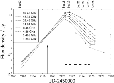
Figure 1: VLA and OVRO Millimeter Array observations of the integrated flux density during the outburst of Cygnus X-3. The bold black horizontal lines indicate the times of the VLBA observations. The arrow indicates the start of the outburst, as detected with the RATAN-600 telescope (Trushkin et al., 2002). Lines have been drawn between the points corresponding to September 9 and September 18, to indicate the change in spectral shape. This does not represent the rate at which the flux density rose during the outburst, as there is insufficient temporal coverage to accurately plot the rise phase of the flare. Note how the spectrum goes from rising with frequency before the flare to falling with frequency afterwards, a trend previously observed as the source moves from the pre-flare “quench” state to outburst (e.g. Fender et al., 1997). A power-law fit to the high frequency decay curves between September 19 and September 23 yields a power-law index of $3.8\pm 0.2$.

The VLBA observations were carried out using dual polarisation and two-bit sampling. At all four frequencies, an 8-MHz bandwidth was used. The two IF pairs were allocated across an uninterrupted frequency range, rather than being more widely spaced. Scans on Cygnus X-3 were interleaved with scans on a phase calibrator source, with a 3-minute cycle time (70 s on the calibrator, 110 s on the source). The calibrators used were J 2052+3635 (5.9^∘ from the source) for September 18 and 19, and J 2007+4029 (4.7^∘ from the source) for all other epochs. The data were correlated using the VLBA correlator in Socorro, New Mexico. All data taken at $<$15^∘ elevation were flagged. Amplitude calibration, fringe-fitting and imaging were carried out using the AIPS software according to NRAO guidelines laid out in Appendix C of the AIPS Cookbook. The flux density scale was set using system temperatures and antenna gains, and is believed to be accurate to $\sim 5\%$ according to the VLBA Observational Status Summary. Fringe-fitting was carried out only on the calibrator sources, not the source itself, except at 22 GHz as described later in this section.

Unfortunately, Cygnus X-3 is one of the most heavily scatter-broadened sources in the radio sky owing to its location in the direction of the Cygnus OB2 association (Wilkinson et al., 1994; Mioduszewski et al., 2001). The size of the scattering disk scales as $\nu^{-2}$, so particularly at the lower observing frequencies, much of the information from the long baselines was lost, and the resulting uv-coverage of the observations was poor. In addition, the images of the phase calibrators themselves were heavily scattered, so it was not possible to calibrate the outer antennas at low frequencies. Only the baselines between the antennas in the southwestern United States (the VLA antenna, Pie Town, Los Alamos and Fort Davies) yielded useful information about the source. This meant that we were unable to produce any good quality images at 1.6 GHz, and that the resolution decreased more markedly with frequency than would have been expected from a simple $\lambda/D$ decline.

In addition to sparse uv-coverage (the VLBA itself has a maximum of ten antennas, the outermost of which were lost owing to the scattering of information from long baselines), the complex, variable nature of the source during each observation posed further difficulties for the data reduction. In an observation of duration 13 hours, the components of the source would not only change in flux density, but would also gradually change position, owing to the motion of the jet during the period of observation. Modelling the latter effect however revealed that the positional changes would simply elongate the components in the images. This effect would in fact only be a problem at the highest frequency, since for a 13-hour observation, a proper motion of $\sim 10$ milliarcseconds (mas) per day would shift the position by 6.5 mas. This is a little smaller than the beam size at 22 GHz (see Table 3), significantly less than the beam size at 15 GHz and much smaller than the size of the scattering disk at 5 GHz. So even at 22 GHz, the effect would be fairly small. The earlier epochs of VLBA data suffered most from source variability, whereas the relatively low surface brightness of the source caused most of the problems during the later observations. On September 22 and 23, we were unable to produce any good images.

Several approaches to producing good quality images of the source were tried. Splitting the observation into small timeranges and imaging each individually in order to reduce the effects of variability and proper motion was found to help for the early observations when the source was bright, but for the later epochs, did not leave enough flux density to make a good quality image of the source. Self-calibration with a point source model was attempted, but this was not found to improve the image significantly. Imaging only the part of the observation where a plot of the amplitude of the short baselines against time was relatively flat, in order to reduce the effects of variability, was again not found to improve the image. Downweighting the central regions of the uv-plane (corresponding to the short baselines) by the use of super-uniform weighting was similarly found to be of limited use, as was the attempt to model the visibilities with Gaussian components. The method that did most to improve the map was to image and self-calibrate the phase calibrator (J 2007+4029), and then to transfer the solutions for amplitudes and phases to the target. Once the solutions had been transferred, some of the methods listed above were applied once more in an attempt to improve the images. Of these, only downweighting the short baselines was found to significantly improve the images. The resulting images are shown in Figure 2. More information on the images (beam sizes, noise levels and exact observation times) is given in Table 3. Only phase self-calibration was used since amplitude self-calibration was not found to improve the images.

The observations at 5 and 15 GHz were phase-referenced to a calibrator (J 2052+3635 or J 2007+4029 as detailed above) in order to preserve positional information. Since self-calibration was carried out on both the phase calibrator and Cygnus X-3 itself, there might still have been some degree of uncertainty in the absolute sky positions of the images. In order to estimate this effect, a check source was imaged, both phase-referenced to the phase calibrator and to itself. The difference in the position of the check source in the two images gave an estimate of the positional uncertainty introduced in the imaging and self-calibration processes. The check sources used were J 2025+3343 for September 18 and 19 and J 2052+3635 for all other observations.

At 22 GHz, the phase calibrator sources were insufficiently bright, and the images could not be phase-referenced. Thus their absolute sky positions are not accurate; an inevitable consequence of the fringing process is that the brightest point in the source becomes the centre of the image. At 15 GHz and 5 GHz however, phase referencing was carried out.

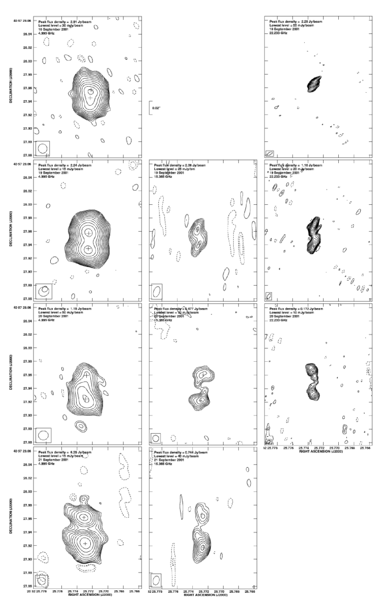
Figure 2: VLBA images of Cygnus X-3 in flare. Images are shown at 4.995 GHz in the left column, 15.365 GHz in the central column, and 22.233 GHz in the right column. Where images are missing, the data were not good enough to make a good quality image. Time progresses down each column, each row a day later than the previous one. Solid contour levels are $(\sqrt{2})^{n}$ times the lowest level stated in the images ($n=0,1,2,\ldots$). Dashed contours are $-1$ and $-\sqrt{2}$ times the stated lowest levels. The beam sizes are shown in the lower left corner of the images. Crosses indicate the fitted positions of the maxima, as plotted in Figure 4. Assuming a distance of 10 kpc to the source, 1 mas on the images corresponds to a projected separation of 10 AU.

6 VLBA image analysis

The linear alignment of features in the VLBA images are interpreted as jets in an almost north-south orientation, in agreement with previous work (e.g. Mioduszewski et al., 2001; Martí et al., 2001).

The total flux densities recovered from the images track fairly well the flux densities measured with the VLA (Figure 3). Perhaps a few hundred mJy is missing at 5 GHz (i.e. $\sim 5$ %), although up to a few Jy (corresponding to several tens of percent) is not recovered at 22 GHz. However, it was difficult to measure accurately the flux densities of the different components from the images, mainly because of insufficient resolution. Hence it was difficult, especially for the images in which the r.m.s. noise is a significant fraction of the component flux density, to derive accurate spectral indices for the emission. At 22 GHz, the northern and southern components (initially unresolved) fade at similar rates, whereas at 5 GHz, the northern component fades more rapidly than the southern component.

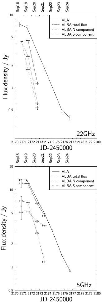
Figure 3: 22-GHz (top) and 5-GHz (bottom) VLBA component fluxes. The total flux detected with the VLBA tracks the flux detected with the VLA fairly accurately. Note how the northern component flux density drops dramatically at both frequencies between September 19 and September 20, a decrease mirrored by the southern component at 22 GHz, but not at 5 GHz. The northern and southern components could not be distinguished at 22 GHz on September 18, and the flux density of the single measured component has been plotted for both, as it was not known how the flux density was split between them.

When considering the images, care should be taken not to overinterpret the details of the structures they show. In the 5-GHz and 15-GHz images, only the gross features should be relied upon, owing to the size of the scattering disk (16 mas at 5 GHz) or the high r.m.s. noise of the images (126 mJy per beam in the 15-GHz image of September 19). The fine structure in the 22-GHz images is certainly believable, owing to the low r.m.s. noise levels achieved and the high resolution of the images (a small beam size and a small scattering disk). Certainly on September 20, the shape of the jet, the extension to the north of the northern maximum, and the double peak to the south are believed to be real.

6.1 Overall morphology

Accepting that the extended emission we observed with the VLBA constitutes a jet, we now consider the nature of the jet; whether it consists of a single pair of ejecta, a continuous set of discrete ejecta, or a continuous hydrodynamic flow.

The lower-frequency and hence lower-resolution (5-GHz and 15-GHz) images show the source to be dominated by two bright components. However, the highest-resolution image at 22 GHz reveals a sequence of several discrete knots, with the flux density being dominated by a single northern component (which we identify in §6.4.2 and §6.4.3 as the core with a northern extension) and a southern component which itself shows hints of being resolved into two distinct peaks. It seems most likely, therefore, that the jet consists of a series of discrete knots, but is dominated by two brighter components; one in the north and one in the south. In most of our subsequent analysis and modelling we concentrate on only the brightest observed components seen at 5 and 15 GHz, since they appear to dominate the flux density of the source and since we believe them to be uncontaminated by core emission (see § 6.4.4). Figure 4 shows the movement of the brightest emitting regions with time.

Assuming the likely nature of the jet as a whole series of discrete ejecta, following the motions of the brightest components can help to determine some of the fundamental jet parameters, e.g. the jet speed (§ 6.2). Measuring the evolution of the sizes of the brightest 22-GHz knots constrains the expansion speed of the plasmons and is evidence that we see discrete blobs. However, by considering the underlying nature of the jet, the positions of all the discrete knots seen in the 22-GHz image from September 20 can be fitted to give information on the way the jet precesses (§ 6.4.3).

6.2 Jet speed

The 15-GHz and 5-GHz data were phase-referenced, and analysis of the positions (depicted in Figure 4) of the two most prominent peaks in the VLBA images suggested that both the northern and southern components had non-zero proper motions. (We chose to ignore the 22-GHz data in these fits because these were not phase-referenced i.e. did not have absolute positional information and, for the reasons described in §6.4.4, because at this high frequency we believe there to be a significant core contribution.) We fitted a straight line to the measured positions at 5 GHz and 15 GHz (both data sets taken together) as plotted in Figure 4 (top and centre). We first constrained the gradient of the northern line to be zero (i.e. a horizontal line, indicating no systematic motion), which fit had a reduced $\chi^{2}$ of 3.8. Fitting for an unconstrained gradient gave a significantly lower reduced $\chi^{2}$ of 0.64, with a best fit value for the proper motion of $2.8\pm 0.5$ mas per day. This is smaller than the best-fit value for the southern component ($8.4\pm 1.7$ mas per day). Assuming the jet is two-sided (which we substantiate in § 6.4), an analysis of the proper motions of the approaching and receding jets (e.g. Mirabel & Rodríguez, 1999) determines $\beta\cos i=0.50\pm 0.10$ (where $\beta=v/c$ and $v$ is the intrinsic speed at which the knots move away from the core, and $i$ is the inclination angle of the jet to the line of sight). This analysis also gives an upper-limit to the distance to the source of $d=35.7\pm 4.8$ kpc and an ensuing upper limit to the inclination angle of the jet axis to the line of sight of $i_{\rm{max}}=59.8\pm 6.7$^∘. Assuming a source distance of exactly 10 kpc, we can solve for the jet speed and inclination angle to get $\beta=0.56\pm 0.09$ and $i=25.7\pm 6.5$^∘.

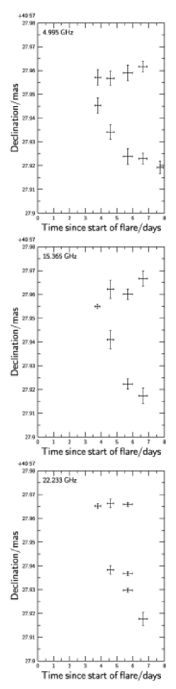
Figure 4: Movement in Declination of the VLBA knots with time. Only Declination is plotted here because the jet axis is very close to north-south (§ 6.4.3 and Mioduszewski et al., 2001) and the knots are expected to move ballistically out from the core. Positions were measured by fitting one or more Gaussians to the emitting regions using the AIPS task JMFIT and finding the positions of the fitted peaks. Fitted positions are shown with crosses in Figure 2. For the points without a corresponding image in Figure 2, the position is taken from the obvious brightest point in a phase-referenced image which had not been self-calibrated. These images had not been included in Figure 2 as we were unable to produce good-quality images for these data sets. Uncertainties in the fitted positions are taken as the canonical value of 25% of the beamwidth. Uncertainties in the time are taken to span the course of each observation. Start of flare is taken as JD $2452167\pm 0.2$ (Trushkin et al., 2002), i.e. 2001 September 14, but see §6.5 for discussion of when the ejection event occurred.

A further check on derived proper motions is often made using a Doppler boosting analysis. Given the fading of the intensities of the plasmons with time (e.g. Figure 3 and § 9.5) a simple Doppler boosting analysis is not valid. A refined application of this method (Mirabel & Rodríguez, 1999) which involves measuring the flux density in the approaching and receding knots at equal angular separations from the core is in this case inapplicable because of the pronounced side-to-side asymmetry which is predicted from the jet speed and inclination angle derived above and which is seen in Figure 5.

6.3 Plasmon size

From the observations, it was possible to derive a maximum size to the source components, which can be used to help estimate the magnetic field in the emitting region. Since the images of Cygnus X-3 are highly scatter-broadened (Wilkinson et al., 1994), particularly at low frequencies, the apparent source size is dependent on frequency. Mioduszewski et al. (2001) reported that the apparent source size scales as

$$\theta=448(\nu/1\,\rm{GHz})^{-2.09}\quad\rm{mas}.$$ (1)

which, within the errors, they found to be consistent with a $\nu^{-2}$ scaling. Thus to determine the true source size, and to obtain the best resolution, we used our highest-frequency (22 GHz) images. The AIPS task JMFIT was used to fit Gaussians to the two brightest knots in the images, and the deconvolved sizes and orientations are shown in Table 4. The quoted sizes do not include a deconvolution from the scattering disk, the size of which is given for the different observing frequencies in Table 3. The observed plasmon sizes increased with time, from $7.9_{-3.0}^{+0.5}$ to $16.9_{-3.6}^{+0.9}$ mas; the errors on these sizes include the apparent elongation due to proper motion of the knots over the course of each observation. For the 8.5-hour observation of September 18, and a derived proper motion of 8.4 mas d^-1, the possible elongation of the knots is of order 3.0 mas. Thus the intrinsic size could be as small as 4.9 mas. What may complicate this simple measurement of the the plasmon size however, is the possibility of there being multiple plasmons, as observed in the September 20 image, which sequentially make a contribution to the observed flux density, but for which the VLBA has insufficient angular resolution. Assuming that the measurements (incorporating the uncertainty due to the smearing effect of component proper motion) do reflect the plasmon expansion, the expansion speed is then $4.6^{+0.8}_{-2.5}$ mas per day, corresponding to a speed of $0.27^{+0.05}_{-0.14}\,c$ for an assumed source distance of 10 kpc. This is, reassuringly, fairly consistent with the plasmon expansion speed of $0.1-0.3c$ fitted by Atoyan & Aharonian (1999) for the 1994 outburst of GRS 1915+105.

6.4 Is the jet one-sided or two sided?

There is some discussion in the literature as to whether the observed jet in Cygnus X-3 is one-sided (owing to Doppler boosting effects reducing the flux density of the receding jet below the map noise as in Mioduszewski et al. (2001)) or two-sided (e.g. Martí et al., 2001). In the following sections, we will try to assess whether the VLBA images of Figure 2 show evidence for a one-sided or a two-sided jet.

6.4.1 Evidence from proper motions

From the proper motion analysis of the 5-GHz and 15-GHz data in §6.2, the fits seem to favour the northern component seen at these frequencies being a moving jet rather than a stationary core. This argues for the observed VLBA jet being two-sided. This conclusion should be taken with the caveat that although the images were phase-referenced, they were also self-calibrated, a process which may in principle move component positions around by a fraction of a beam. Given that the beam size at 5 GHz is between 13 and 16 mas and the northern component is seen to move by 12 mas over the course of the observations, the observed movement could in principle have been caused by the self-calibration. We believe however that the systematic increase in declination of the northern component seen over a number of days at both frequencies is indicative of real proper motion.

6.4.2 Core position

Mioduszewski et al. (2001) showed convincing evidence that the northern component they observed during the 1997 February flare was a core, rather than a receding counterjet to the extension seen to the south. The position of this core in their images appears to be 20^h32^m25^s.7733 +40^∘57^′27^′′.965 (J 2000). Comparing this with the positions in our images shows it to be almost coincident with the maximum in the northern component of the 22-GHz image from 2001 September 20. This would seem to argue that this component in our image (labelled “C1” in Figure 5) is the core. However, Mioduszewski et al. stated that their phase referencing was not entirely successful, so there is some small uncertainty in their derived position (although their images prior to self-calibration showed that the northern component was stationary to within 3 mas). Moreover, the 1997 February outburst was 4.5 years earlier than that of 2001 September. If the system had a systematic velocity (owing to, for instance, a natal kick) of 100 km s^-1, it would move a distance $\approx 95$ AU in 4.5 years. If this motion were in the plane of the sky, that would imply a shift in position of 10 mas at the distance of Cygnus X-3. That this should be along the jet axis is unlikely, but it should be borne in mind that the source core position might in principle have changed in the intervening time between the outbursts.

6.4.3 Jet precession and modelling

The final 22-GHz image (from September 20) shows a series of emitting knots, and the brightest northern component is coincident with the position of the core as determined by Mioduszewski et al. (2001). We attempted to fit the precessing jet model of Hjellming & Johnston (1981) to this image, investigating the three most plausible core positions, corresponding to the brightest point in the northern component (at 20^h32^m25^s.77335 +40^∘57^′27^′′.9650), the flux density peak immediately south of that (at 20^h32^m25^s.77315 +40^∘57^′27^′′.9555), and the flux density peak at the centre of the jet flow (at 20^h32^m25^s.77295 +40^∘57^′27^′′.9487), all given in J 2000 co-ordinates. These positions correspond to the points labelled “C1”, “C2”, and “C3” respectively in Figure 5. We used a minimisation routine based on the downhill simplex method (Press et al., 1992) in order to find the best agreement between the model and the image. The precessing jet model has eight independent parameters: the inclination of the jet axis to the observer, $i$; the opening angle of the precession cone, $\psi$; the angle through which the jet is rotated in the plane of the sky from an E-W alignment, $\chi$ (related to the position angle by P.A. $=\chi+90$^∘); the source distance, $d$; the jet speed $\beta c$; the precession period, $P$; the sense of precession $s_{\rm rot}$ (clockwise or anticlockwise); and some initial phase of precession, $\phi$. We added in an extra parameter $t_{\rm view}$, the time after ejection at which the image was made. We measured the positions and flux densities at fifteen different points along the spine of the jet, and then weighted the points according to the corresponding flux densities. It was found that a simple minimisation of the sum of the weighted distances between each measured jet position and the closest model point did not give reasonable solutions, since the minimised model parameters would predict radio emission from points well outside the observed jet. To improve the fits, additional terms were used in the function to be minimised, penalising a fit if it predicted too many precession periods to have passed in the time between ejection and observation, and penalising it if it predicted radio emission outside a small box containing the observed jet. The minimisation routine was run for almost a hundred thousand different sets of starting parameters, which were chosen in order to fully sample (at equal intervals) the available parameter space without taking a prohibitively long time to run. Results predicting $\beta>1$, distances outside the range $5<d<15$ kpc (Predehl et al., 2000; Dickey, 1983), or negative periods were disallowed. The sum of the distances from each jet position to the closest model point was computed for each of the converged results, and the results with the lowest such cumulative distances which also predicted a viewing time $t_{\rm view}<8.5$ days (the time between the detection of the initial rise of the radio flux density and the epoch at which the image was made) were then examined individually, to check that the results with the lowest cumulative distances did in fact produce good by-eye fits to the data. Upon examination, no satisfactory fits were found for core positions corresponding either to the centre of the jet flow (core position C3), or to the southern part of the northern component (C2). However, good by-eye fits to the data were found for a core position corresponding to the brightest point in the north component (C1). We therefore identify the brightest point in the northern component as the core of the system.

For that northernmost core position, more good fits were found for clockwise rotation ($s_{\rm rot}=-1$) than for anticlockwise rotation ($s_{\rm rot}=+1$), and the mean, standard deviation, and the maximum and minimum values for the satisfactory fits are given in Table 5. The sense of the jet precession can not be uniquely determined in this case, but the parameters $\psi$, $\beta$, $P$, and $t_{\rm view}$ are similar for the two possible senses. $\phi$ and $d$ are not uniquely determined, with $\phi$ having a large standard deviation and the distance varying between the limits allowed by the model-fitting code. Although the parameters $i$ and $\chi$ appear very different in the two cases, we believe that this is due to the way the angles were defined in the model of Hjellming & Johnston (1981). In changing the sense of jet precession from clockwise to anticlockwise, all angles will be measured in the opposite sense, which will affect the definitions of inclination angle and position angle on the sky. Redefining $i_{\rm new}=180-i$ and $\chi_{\rm new}=\chi-180$ for the anticlockwise case gives $i_{\rm new}=10.4\pm 3.8$ and $\chi_{\rm new}=98.1\pm 2.8$, in good agreement with the parameters derived for the clockwise case. So, taking the core position to be at 20^h32^m25^s.77335 +40^∘57^′27^′′.9650, as allowed by the fits, we can constrain the system parameters to be $\psi=2.4\pm 1.2$^∘, $i=10.5\pm 4.2$^∘, $\chi=98.9\pm 2.9$^∘, $\beta=0.63\pm 0.09$, and $P=5.34\pm 0.67$ days. This gives a value $\beta\cos i=0.62\pm 0.11$. Comparing this value with that of $\beta\cos i=0.50\pm 0.10$ derived from the proper motion analysis of § 6.2, we find a slight discrepancy, although the error bars do overlap. Our best model fits for both senses of precession are shown in Figure 5. We cannot robustly determine the sense of precession with this data.

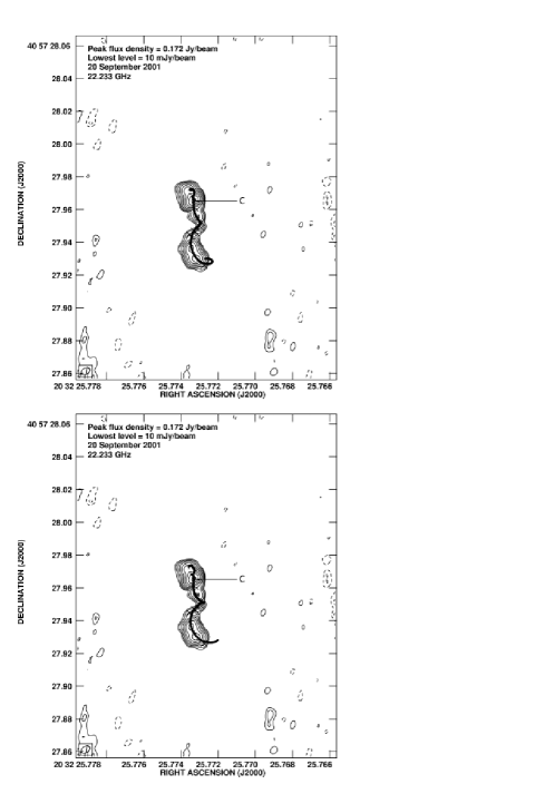
Figure 5: Results of fitting the model of Hjellming & Johnston (1981) to the 22-GHz VLBA image of September 20. The black dots overlaid on the VLBA image correspond to the derived positions of knots ejected every 0.1 days from the core. The bottom image is for clockwise rotation ($s_{\rm rot}=-1$) and the top image for anticlockwise rotation ($s_{\rm rot}=+1$). Both models fit all the major peaks in the southern jet, the direction of the northern jet, and the approximate lengths of the two jets. They make no allowance for the fading of jet knots with time.

Thus we do see a two-sided jet on VLBA scales. However, the jet speed $\beta$ and the inclination angle $i$ are such that the observed length of the northern jet is significantly shorter than that of the southern jet. The ratio of the arm lengths is

$$\frac{l_{\rm{app}}}{l_{\rm{rec}}}=\frac{1+\beta\cos i}{1-\beta\cos i},$$ (2)

where $l_{\rm{app}}$ is the length of the approaching jet and $l_{\rm{rec}}$ is the length of the receding jet, $\beta$ is the jet-knot advance speed, and $i$ the inclination of the jet axis to the line of sight. The fitted parameters in the precession model imply a length ratio of $4.3\pm 0.3$. Figure 5 shows that the north jet is indeed shortened by a factor appropriate to these values of $\beta$ and $i$, convincingly verifying the two-sidedness of the jet in Cygnus X-3 on this occasion.

6.4.4 VLBA component spectra

The flux densities of the source components (shown in the images of Figure 2) during the flare of 2001 September were measured using the AIPS task JMFIT. The 5-GHz VLBA component lightcurves are shown in Figure 3. The total emission (the sum of the northern and southern components) was found to track the VLA flux density. At 5 GHz, the integrated flux density of the northern component exceeded that of the southern component on September 18 and 19, after which its flux density diminished more rapidly, and the southern component dominated. At 22 GHz, the northern and southern components could not be distinguished on September 18. On September 19, the northern component dominated, and the flux densities of the two components were comparable on September 20. When the spectral indices of the VLBA components were determined, it was found that neither component had an flat or inverted spectrum between 5 GHz and 22 GHz. Figure 5 shows that the core and the northern (receding) jet are very close together owing to relativistic aberration, and therefore would not be resolved at 5 GHz. It is the jet which dominates the flux density at low frequencies (5 GHz and 15 GHz), but the core dominates at 22 GHz because it has a significantly less steep spectrum than the jet material. Therefore spectral indices between these frequencies will not (without significantly higher resolution) reveal the identity of the northern emission, be it core or jet.

6.5 Is the ejection of the VLBA emitting regions coincident with the start of the VLA flare?

The time of the beginning of the radio outburst can be constrained to being on or prior to JD 2452167 (2001 September 14), from the RATAN-600 data (Trushkin et al., 2002), and from Ryle Telescope monitoring (Pooley, 2001). The Ryle Telescope monitoring shows that the 15-GHz flux density began to rise out of the pre-outburst “quench” period from 0.02 Jy on JD 2452162.5 to 0.1 Jy by JD 2452165.

Extrapolating the positions of the VLBA knots at 15 GHz and 5 GHz (the absolute 22-GHz positions being inaccurate due to the lack of phase-referencing) in Figure 4 backwards in time, we believe that those knots cannot have been ejected at the time when the low-resolution telescopes (the RATAN-600 and the VLA) detected the radio flux density beginning to rise. Extrapolating to a precise time of ejection is difficult, owing to the large uncertainties on the measurements, but it seems that the northern and southern components would have been coincident perhaps $2.5\pm 0.5$ days after the RATAN-600 saw the radio flux density start to rise at the beginning of the outburst. This is $1.3\pm 0.5$ days prior to the first VLBA observation on 2001 September 18. By way of explanation, we propose a scenario in which the core flared and only expelled the jets later. This we explore in a forthcoming paper. Note that this is the opposite order of events to that proposed by Atoyan & Aharonian (1997), who suggested a scenario whereby the radio flux density flared well after the ejection of radio clouds, once they had expanded sufficiently to become transparent at radio frequencies. Alternatively, it may be that the jet speed increased over the course of the first few days, although we note that once VLBA monitoring began (on September 18) the positions of the knots are consistent with a constant separation velocity, suggesting that their motion has always been ballistic.

6.6 Comparison with previous work

The most detailed previous VLBI images of Cygnus X-3 were made by Mioduszewski et al. (2001). They made three observations at 15.365 GHz with the VLBA at epochs 2, 4, and 7 days after the peak of a 10 Jy radio flare in 1997 February. Mioduszewski et al. detected what they interpreted as a stationary (to within 3 mas) core component and a continuous jet extending to the south, reaching a maximum observable extension of 120 mas four days after the flare, which faded beyond the detection limits by the last observation. They took the time of ejection of the radio-emitting plasma to be the start of the outburst as detected by the Ryle Telescope and the Green Bank Interferometer (GBI), and from the measured lengths of the jet at different epochs, derived proper motions, which constrained the jet speed to be $\beta_{\rm{min}}\gtrsim(0.78-0.75)$, and a weak upper limit to the inclination to the line of sight to be $i<78$ ^∘. Then, from the ratio of the integrated flux density in the southern jet to the integrated noise in the north taken over a smaller area (to account for slower apparent motion of the receding jet), they derived a constraint on $\beta\cos i\gtrsim 0.806$. We believe that there is some scope for error in their proper motion analysis, since it rested on the length of the jet, rather than on tracking individual well-identified knots of radio emission. The length of a jet that may be imaged will be affected by the map quality, which was poor during at least the first epoch of their observations, owing to bad weather in the southwestern USA. Moreover, it is not clear that the radio plasma was ejected at the start of the Ryle/GBI flare (see §6.5). Uncertainty in the ejection time would then lead to an error in the proper motion and the derived jet speeds.

A comparison may also be made between the precession parameters derived for the 1997 flare and those we derived in § 6.4.3. Their best fits yielded a precession period $\gtrsim 60$ days, a jet speed $\beta\gtrsim 0.81$, a precession opening angle of $\lesssim$12^∘, an inclination angle of $\lesssim$14^∘ to the line of sight, and anticlockwise precession. The inclination angle, jet speed and opening angle derived by Mioduszewski et al. (2001) were similar to those we derived.

Because the derived precession period of the 2001 event is comparable to the monitoring timescale (c.f. the 1997 event, when the monitoring sampled less than one tenth of the best-fit precession period), we have confidence in the limits we have placed on this parameter. However, the fits of Mioduszewski et al. robustly require a long precession period ($\gtrsim 30$ days), whereas ours is of order $\sim 5.3$ days. It is thus hard to avoid the conclusion that the precession period has changed by a significant factor between these two events.

From the above, we believe that the jet speed we derive from proper motion measurements is consistent with that estimated by Mioduszewski et al. (2001). In both sets of observations, the southern jet appears to be brighter and faster-moving than any northern jet and in both sets of data there is evidence for precession (albeit with rather different precession parameters). In addition, the nature of the jet itself appears to be different, in the sense that the 2001 September jet seemed to be composed of a few identifiable knots, whereas the 1997 February jet appeared more like a continuous stream of radio plasma. On the other hand, intrinsic differences could, in principle, account for the difference in the observed nature of the jet. The outburst of 1997 February was shorter in duration than that of 2001 September. The integrated flux density died away more quickly in the 1997 flare (falling to below 1 Jy at 15 GHz $\sim 3$ days after the peak of the flare, as compared to $\sim 5$ days afterwards in 2001), after which it was still possible to make VLBA observations. The dynamic range-limited images of Mioduszewski et al. therefore have much lower r.m.s. noise levels than those in Figure 2, so lower-level continuous emission (as opposed to the discrete knots we observed) could be detected. This could account for our non-detection of continuous emission, although the comparison of VLA and VLBA flux densities suggest that we are not missing significant components in our VLBA images, at least at low frequencies.

A comparison may also be made to the flare of 2000 September 15 observed by Martí et al. (2001). They observed Cygnus X-3 with the VLA in its most extended “A” configuration 36, 51, and 66 days after the start of a radio outburst detected with the GBI. By this latest time, the source had faded back to quiescence. They imaged a two-sided ejection on arcsecond scales, with a dominant core, a prominent northern ejection and a strong hint of extension to the south. The flare observed with the GBI was less powerful than either the 1997 or the 2001 flare, peaking at only $\sim 7$ Jy at 8.3 GHz.

Martí et al. (2001) derived proper motions by assuming the ejection date to be the start of the flare observed with the GBI, and obtained a value of $\beta\cos i=0.14\pm 0.03$. In fact, their plot of the GBI data shows several flares of amplitude $>4$ Jy over the 20 days following their assumed ejection date (after which no data is plotted, since GBI monitoring of Cygnus X-3 appeared to cease on JD 2451821). This opens up two possibilities. It is not clear which (if any) of the plotted flares was associated with the actual ejection event corresponding to the jets they observed. If the last one (JD 2451822) was the flare responsible, their third image showing the arcsecond-scale jets would have been taken only 46 days after the flare. This would lead to increased values for the proper motion of the two jet components, and a derived jet speed of $\beta=0.68$. It is also possible that the ejection occurred after their GBI data stops, in which case the derived proper motions and speeds would be even greater. A speed of $\beta=0.68$ is much more consistent with that derived in this paper. It is not clear however that the expansion rate would be uniform and it is possible that the jet would slow down as it impinged on its environment. While this effect might be negligible over a few days, it might be significant on a timescale of months. However, their value of $\beta\cos i=0.12\pm 0.01$ based on the flux density ratio of the 2 jets interpolated to equal angular distances from the core would seem to be more robust than the value derived from their proper motion analysis.

Martí et al. explained the one-sided VLBA jet observed by Mioduszewski et al. (2001) by invoking jet obscuration by an absorbing medium on VLBA scales, in the form of a free-free absorbing disk-like wind. They suggested that the northern jet was the approaching jet, and the southern jet was receding from us. For the 15-GHz images of Mioduszewski et al., they derived an optical depth at 50-100 mas from the core of $\tau_{\nu}^{\rm{ff}}=1.15\pm 0.14$. Since their quoted free-free absorption coefficient scales as $\nu^{-2.08}$, that would imply an optical depth of $0.53\pm 0.08$ at 22 GHz. This would be insufficient to prevent us from seeing a bright approaching northern jet in our images. Since our observations strongly suggest a receding northern jet, it would be hard to reconcile their obscuration explanation with our data.

We made further observations of Cygnus X-3 134 days after the detected start of the 2001 September flare, on 2002 January 25, whose detailed analysis we will present in a forthcoming paper. As with the observations of Martí et al., the VLA was in “A” configuration, and the source had faded back to a quiescent flux density of $\approx 100$ mJy at 43 GHz, although it displayed significant variability on a timescale of $\approx 10$ minutes. We subtracted out the time variability, and then imaged the core. Fitting that with a Gaussian and subtracting this from the uv-data set, there was no evidence of any extension similar to that seen by Martí et al., to an r.m.s. limit of 0.8 mJy per beam. We note, however, that this is as expected, since Martí et al. (2001) detected northern and southern extensions 66 days after the assumed ejection event (see discussion above) at levels of 1.45 mJy and 0.89 mJy respectively. Assuming that the flux densities of these extensions decreased with time, then 134 days after the start of the outburst, such extensions would be undetectable at our r.m.s. limit.

7 Radio spectra

7.1 General characteristics

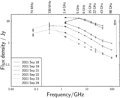
Figure 6: Evolution of the radio spectrum of Cygnus X-3 

The high-frequency parts of the spectra shown in Figure 6 were fitted with single power laws and the resultant spectral indices are shown in Figure 7. The spectral index evolved during the course of the flare, from a value of $0.44\pm 0.06$ on September 18 to a value of $0.61\pm 0.08$ by September 23. Traditional models of synchrotron radiation cannot explain such a spectral steepening, although this phenomenon has been seen before, in the giant radio outburst of 1972 (Aller & Dent, 1972; Hjellming & Balick, 1972; Peterson, 1973), and in subsequent outbursts (e.g. Seaquist et al., 1974; Geldzahler et al., 1983).

The spectra also show that by September 24 (if not earlier), the spectra began to deviate from pure power laws, and rapid variability began to affect the source flux. Two different scans were made at 8.4 GHz on September 24, each of duration 2 minutes, and separated by 30 minutes (this was the only epoch when separated scans were made); in this time, the source flux density increased from $618.2\pm 1.2$ mJy to $656.5\pm 1.2$ mJy. The main outburst dominated the source flux during the first few days of observation, but as the outburst decayed, the source behaviour was affected more by core variability or minor ejections.

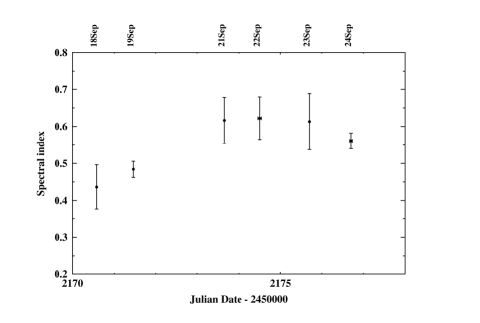
Figure 7: Evolution of the spectral index of Cygnus X-3. The spectral index was fitted with a simple power-law for the portion of the spectrum that was well above the low-frequency turnover ($>8.4$ GHz for September 18 and 19, $>5$ GHz for September 21 and 22, and $>1.4$ GHz for September 23 and 24).

7.2 What causes the low-frequency turnover?

The low-frequency (1.4-GHz to 74-MHz) measurements indicate a turnover in the radio spectrum. We now consider various possible mechanisms for creating such a turnover, and assess the plausibility of each one. Such low-frequency turnovers in other sources are generally ascribed to one of four distinct mechanisms (Kellermann, 1966; Gregory & Seaquist, 1974). These are: synchrotron self-absorption (SSA), a low-energy cutoff in the electron energy distribution spectrum, the Tsytovich-Razin (T-R) effect, and free-free absorption (FFA) by thermal plasma, either with the plasma uniformly mixed with the radiating electrons or as intervening material along the line of sight to the source. We now discuss these four possibilities in turn.

7.2.1 Synchrotron self-absorption

Well below the turnover frequency $\nu_{\rm m}$, where the optical depth $\tau\gg 1$, a synchrotron self-absorbed spectrum scales as $S_{\nu}\propto\nu^{5/2}$ (e.g. Rybicki & Lightman, 1979). In the optically-thin region however, where $\tau\ll 1$, the scaling is $S_{\nu}\propto\nu^{-\alpha}$ ($\alpha>0$). The width of the turnover region depends on the structure of the source. Unfortunately, we do not sample the low-frequency spectrum well enough to determine whether the terminal low-frequency spectrum scales as $\nu^{5/2}$. However, we clearly observed that the turnover moved to lower frequencies with time. If the synchrotron self-absorption paradigm is correct, this would be consistent with the observed expansion of the plasmons, which would cause the magnetic field within the plasmons to decline, and thus lower the turnover frequency. Magnetic flux freezing implies that $B/\rho\propto\Delta l$ (Landau & Lifshitz, 1963), where $\rho$ is the plasma mass density, $B$ is the magnetic flux density, and $\Delta l$ is the length of a fluid element along the magnetic field line. Assuming that the mass of the plasma cloud is constant and that there is no strong turbulence, $\Delta l(t)\propto R(t)$, and $B\propto R^{-2}$. However, if turbulence develops in the plasma, the fluid elements are stretched by turbulent eddies in addition to the expansion of the cloud, so $\Delta l\propto R^{1+\alpha}$, where $\alpha$ in this case is a factor describing the degree of turbulence, typically taken as of order 1 for a turbulent plasmon with a correspondingly tangled magnetic field. In this case, $B\propto R^{-2+\alpha}\approx R^{-1}$. So as the plasmon expands, the magnetic field declines, and the turnover frequency decreases. Thus the SSA scenario is consistent with our data.

7.2.2 Low-energy cutoff in the electron spectrum

We modelled the electron distribution as a power law. If that power law were to extend only down to some minimum energy, below which the electron distribution turned over, producing a cutoff in the electron distribution function, that would produce a low-frequency turnover in the radio spectrum. This turnover would move to lower frequencies as the energies of the individual electrons decreased due to adiabatic expansion of the plasmon, moving the cutoff in electron energies to lower energy. We cannot rule out this possibility with our data. Depending on the abruptness of the cutoff, observing a $\nu^{1/3}$ spectrum below the turnover would identify this scenario.

7.2.3 The Tsytovich-Razin effect

The refractive index, $n$, of a plasma containing free electrons and ions may differ from unity and signals then travel at the phase velocity $c/n$. In a medium where the refractive index is less than one, beaming from relativistic electrons is suppressed, as the angle into which the radiation is beamed is given by

$$1/\gamma=\sqrt{1-n^{2}\beta^{2}}.$$ (3)

At low frequencies ($\nu\ll\nu_{\rm{p}}$, where $\nu_{\rm{p}}$ is the plasma frequency), this effect is dominant, and the synchrotron spectrum is cut off due to beaming suppression. At higher frequencies, this effect is unimportant, since

$$n^{2}=1-\left(\frac{\nu_{\rm{p}}}{\nu}\right)^{2}.$$ (4)

The frequency in GHz at which this effect becomes significant is given by

$$\nu\sim 2\times 10^{-14}n_{\rm{th}}/B,$$ (5)

where $B$ is the magnetic field in Gauss and $n_{\rm{th}}$ is the density of ambient thermal matter in m^-3. In § 8.1 we estimate an upper limit on the magnetic field to be $B\sim 0.15$ G; thus if the T-R effect were the mechanism by which the spectrum turns over, a rather high (upper limit to the) density of $8\times 10^{12}{\rm m}^{-3}$ of thermal plasma would be required for a turnover frequency of 1 GHz. At these densities, free-free absorption would also be expected to become important.

7.2.4 Free-free absorption

We consider two possible geometries for free-free absorption. The absorbing thermal material could either form a screen enclosing but not permeating the source, or it could be mixed in with the synchrotron-emitting plasma.

In the former case, if the plasmons were expanding into a region of thermal material, then the flux of the receding component would fall off more rapidly with time than the flux of the approaching component, since the length of the absorbing screen would increase as the receding plasmon moved away from the core. The length of the absorbing screen between the observer and the approaching component would decrease with time, so the turnover would move to lower frequencies with time as this component began to dominate the observed flux density. In fact, we see evidence that the 5-GHz flux density of the northern (jet) component falls off rapidly with time after September 19, whereas that of the southern component does not diminish so rapidly. This is then in principle a plausible scenario.

For thermal material to be mixed with the synchrotron-emitting plasma, the material would either need to be present at the time the plasmon was ejected, or would have to be entrained during the subsequent motion of the plasmon through the surrounding medium. In order to create a turnover at frequencies as high as $\sim 3$ GHz by September 18, the initial rate of entrainment would have to be extremely high. To cause the observed decrease in turnover frequency, the rate would then have to be quite accurately tuned. We do not favour this explanation.

7.2.5 Discussion on the origin of the turnover

The change in turnover frequency with time places more stringent constraints on the mechanism responsible for the turnover. For the T-R effect, the change in turnover frequency with time would require a change in $n_{\rm{th}}/B$. For FFA, it requires a decreasing density with time, either due to the source moving into lower-density regions as it moves outwards, or due to the expansion of thermal material mixed in with the synchrotron-emitting electrons. For SSA, expansion and a corresponding decrease in the magnetic field lead to a decrease in the absorption coefficient and therefore in the turnover frequency. Multi-frequency imaging with sufficiently high resolution at or below the turnover frequency could in principle distinguish definitively between the mechanisms.

7.3 High-frequency spectral evolution

In order to explain the high-frequency spectral evolution, in § 9, we develop a model which factors in light travel time effects both within and between components, which we believe explains the basic characteristics of the spectral evolution, e.g. the observed timescale. But first we derive some basic parameters of the source in § 8.

8 Constraining the magnetic field and Lorentz factors

8.1 Magnetic Field

If self-absorption were the mechanism responsible for the turnover, precise size constraints from VLBA measurements would allow the direct determination of the magnetic field. If, however, another process were responsible, the self-absorption turnover frequency $\nu_{\rm m}$ would be at a lower frequency than the observed turnover in the spectrum. Thus an extrapolation of the power-law spectrum back to the predicted self-absorption turnover frequency would give a higher extrapolated turnover flux density $S_{\rm m}$ than is observed. Since $B\propto S_{\rm m}^{-2}\nu_{\rm{m}}^{5}$, assuming that the observed turnover frequency and flux density are due to SSA still gives an upper limit to the magnetic field strength.

Assuming that the turnover in the spectrum of Cygnus X-3 is due to SSA, then given the frequency, $\nu_{\rm{m}}$, and flux density, $S_{\rm{m}}$, of the turnover, and the angular size $\theta$ of the emitting region, synchrotron theory gives an expression for the magnetic field in that region (Marscher, 1983).

$$B=10^{-5}b(\alpha)\theta^{4}\nu_{\rm{m}}^{5}S_{\rm{m}}^{-2}\left(\frac{\delta}{1+z}\right)\textrm{G},$$ (6)

where $S_{\rm{m}}$ is measured in Jy, $\theta$ in milliarcseconds and $\nu_{\rm{m}}$ in GHz. The parameter $b(\alpha)$ is a slowly-varying function of the high-frequency spectral index with a value of $\approx 3.4$ for $\alpha=0.6$, and $\delta$ is the beaming parameter

$$\delta=\frac{1}{\Gamma(1-\beta\cos i)},$$ (7)

where $\Gamma$ is the bulk Lorentz factor, $(1-\beta^{2})^{-1/2}$. The redshift $z$ is zero.

Using the VLBA observations to constrain the number and sizes of synchrotron-emitting components, it is possible to fit spectra to those components and derive upper limits to their magnetic fields. Unfortunately, the strong dependence of the magnetic field on the angular diameter $\theta$ and the turnover frequency $\nu_{\rm{m}}$ means that the uncertainty in the derived field is quite high. It also makes it extremely important to define correctly the angular diameter $\theta$. The radiative transfer equation used to derive Equation 6 assumes spherical components. The fitting task in AIPS used to derive the sizes models the components as elliptical Gaussians. Marscher (1987) gives an expression for the value $\theta_{\rm{s}}$ of a sphere which subtends the same solid angle as an ellipse of major and minor FWHM axes $\theta_{\rm{G_{a}}}$ and $\theta_{\rm{G_{b}}}$ as

$$\theta_{s}=1.8\sqrt{\theta_{\rm{G_{a}}}\theta_{\rm{G_{b}}}}.$$ (8)

These equivalent angular sizes are listed in Table 4. Using Equations 6 and 8, together with the fitted turnover frequency of $3.01\pm 0.06$ GHz, the turnover flux density of $15.1\pm 0.5$ Jy, the spectral index of 0.4, and the measured core size of $7.88\pm 0.51$ mas on September 18 (when the VLBA observations suggest that the source consisted of a single component; we note that even if it did not, the individual component sizes would then be smaller than the fitted size, which we could therefore still use to place a reasonably firm upper limit on the magnetic field), an upper limit on the magnetic field of $1.5\pm 0.6\times 10^{-1}$ G ($1.5\pm 0.6\times 10^{-5}$ T) is derived.

This is our best estimate of the magnetic field strength. It could, however, be at least an order of magnitude lower. The proper motion of the plasmons during the course of a VLBA observation would elongate the observed knots in the images and cause us to overestimate their sizes. If this effect were taken into account, the derived magnetic field might be at least as low as $1.94\pm 0.96\times 10^{-2}$ G.

8.1.1 Equipartition?

If the particle and magnetic field energies in the source components were close to equipartition, it would be possible to estimate the minimum-energy magnetic field in the plasmon. Following the derivation set out in Longair (1994), and using measurements of the flux densities and plasmon sizes (Table 4) from September 18, and assuming a factor of 100 times more energy in relativistic protons than in electrons, this assumption gives a minimum-energy magnetic field of $6\times 10^{-2}$ G, corresponding to a minimum energy in the plasmon of $3\times 10^{34}$ J (an energy density of $4\times 10^{-5}$ Jm^-3). Since our upper limit on the magnetic field is greater than the minimum-energy field, our measurements are not necessarily inconsistent with equipartition (although we note that there is no compelling reason why the equipartition assumption should hold in such a manifestly non-steady state system).

8.1.2 Comparison to other magnetic field estimates

Most derivations of the magnetic field in microquasar jets come from equipartition arguments, despite the uncertainty as to whether equipartition is valid in these systems. Spencer et al. (1986) used equipartition arguments to put a lower limit of 0.08 G on the magnetic field of the emitting components during the 1983 September outburst of Cygnus X-3. Equipartition assumptions applied to other sources have also led to minimum-energy magnetic fields of order $0.01-1$ G (for instance GRS 1915+105 (Atoyan & Aharonian, 1999), LS 5039 (Paredes et al., 2000), and Scorpius X-1 (Fomalont, Geldzahler & Bradshaw, 2001)).

A few magnetic field estimates are available in the literature which do not rely on equipartition. Ogley et al. (1998) used electron ageing arguments to put an upper limit on the magnetic field in the jet of Cygnus X-3 in quiescence of $B\leq 20$ G at $5\times 10^{12}$ cm from the core. Paredes et al. (2002) considered inverse Compton processes from a conical jet to constrain the magnetic field at 1000 AU from the core of LS 5039 to lie between 0.06 and 128 G. Thus our estimate of the magnetic field in Cygnus X-3 is consistent with derived values in both this system and in other microquasars.

8.2 Lorentz factor

To a good approximation the radiation observed at a given frequency $\nu$ probes electrons of Lorentz factor

$$\gamma=\left(\frac{2\pi m_{\rm{e}}\nu}{eB}\right)^{1/2},$$ (9)

where $B$ is the magnetic field in T, $\nu$ the observing frequency in Hz, and the constants are in S.I. units. In the case of adiabatic expansion, the magnetic field decreases as the source expands, and observations at a fixed frequency sample electrons with higher Lorentz factors.

From the derived upper limit to the magnetic field on September 18 of 0.15 G, and the maximum and minimum observing frequencies on that day (43.3 and 1.4 GHz respectively), the lower limits to the Lorentz factors of the electrons probed by the measurements are 321 and 58 respectively.

8.3 The $B-\gamma$ plane

Synchrotron theory, taken together with our data, can be used to derive constraints on the area of the $B-\gamma$ plane (Figure 8) occupied by the source in 2001 September.

8.3.1 Synchrotron self-absorption turnover

The upper limit on the magnetic field derived in § 8.1 from synchrotron self-absorption arguments is shown as line 1 in Figure 8.

8.3.2 Energetics

If we assume that the energy ejected during the outburst cannot greatly exceed the energy emitted by a body radiating at the Eddington luminosity over the rise time of the outburst (taken to be of order 1 day), then an upper limit on the total energy in the plasmon should be of order $\sim 10^{36}(M/M_{\odot})$ J. This energy is contained in the relativistic particles and the magnetic field. An upper limit to the magnetic field can be found if all the energy is assumed to be in the field rather than the particles. Knowing the volume of the plasmon (assumed spherical) on September 18, this leads to a limit on the energy density of $10^{-3}(M/M_{\odot})$ Jm^-3. By measuring the Doppler shifts of X-ray spectral lines, Stark & Saia (2003) placed an upper limit on the mass of the compact object of $3.6$ $M_{\odot}$(subject to certain assumptions). Thus an upper limit of $6\times 10^{-1}(M/M_{\odot})^{1/2}=1.1\,$ G may be placed on the magnetic field (shown as line 2 in Figure 8).

8.3.3 Absence of catastrophic synchrotron losses

The fact that the spectrum shows no noticeable break up to 100 GHz implies that synchrotron losses cannot be important up until at least the time of the last observation on September 24. The flare began on September 14. Thus the synchrotron loss timescale $t_{\rm{syn}}$ must exceed ten days. This puts a limit on $B^{2}\gamma$, namely

$$B^{2}\gamma<8.9\times 10^{2}\quad\rm{G^{2}}.$$ (10)

This is shown as line 3 in Figure 8.

8.3.4 Lack of leakage

Another constraint may be derived by considering the synchrotron-emitting electrons. To emit synchrotron radiation, they must be gyrating in a magnetic field. In order for the electrons to remain within the plasmon (where the magnetic field is high enough for them to produce detectable radio emission), their gyroradius must be significantly smaller than the size of the plasmon. If it becomes too large, electrons will begin to leak out of the plasmon and will no longer produce detectable emission. The gyroradius $r_{\rm{g}}$ of an electron of Lorentz factor $\gamma$ in a field $B$ is

$$r_{\rm{g}}=\frac{\gamma m_{\rm{e}}c}{eB}.$$ (11)

Requiring this to be less than some fraction $f$ of the size of the plasmon gives

$$\frac{\gamma m_{\rm{e}}c}{eB}<f\theta d,$$ (12)

where $\theta$ is the observed angular size of the plasmon and $d$ is the distance to the source (taken as 10 kpc). This limit is shown as line 4 in Figure 8.

8.3.5 Region probed by the measurements

Since the electrons radiate at particular frequencies, Equation 9 can be used to find the exact lines on the $B-\gamma$ plane probed by the observations at each frequency (shown as lines 5 in Figure 8).

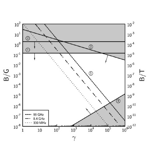
Figure 8: Constraints on the $B-\gamma$ plane. 1 is the upper limit on the magnetic field from SSA (Equation 6) and the size constraint of 7.7 mas from VLBA observations (§ 8.3.1). 2 is the constraint from energetics considerations assuming a 3.6 solar mass compact object (§ 8.3.2). 3 is the synchrotron ageing limit from Equation 10 (§ 8.3.3). 4 is the limit from the requirement for the gyroradius to be less than 10% of the plasmon size, for an angular size of 7 mas (§ 8.3.4). 5 are the loci in the plane probed by observations at three given frequencies (Equation 9). Dashed lines are for 99 GHz, dot-dashed lines for 8.4 GHz and dotted lines for 330 MHz. The arrows show which side of the constraint lines are valid parameter space. The shaded areas denote parameter space which is excluded.

8.4 Number and energy densities

From Longair (1994) and integrating over a power-law distribution of electrons with exponent $p\neq 2$ (in acknowledgement of the terminal high frequency spectral indices we observe, even though $p=2$ is the most frequently-quoted case as it simplifies the mathematics) an expression for the number density of emitting electrons may be derived. Modelling the emitting region as a sphere of uniform density, of radius $r=\text@frac{1}{2}\theta d$, the number density (in m^-3) of emitting electrons is

$$n_{\rm{e}}=\frac{24S_{\nu}(m_{\rm{e}}c^{2})^{1-p}(\gamma_{\rm{min}}^{1-p}-\gamma_{\rm{max}}^{1-p})}{2.344\times 10^{-25}(p-1)d\theta^{3}a(p)\left(\frac{B}{10^{4}}\right)^{\frac{p+1}{2}}\left(\frac{1.253\times 10^{37}}{\nu}\right)^{\frac{p-1}{2}}}$$ (13)

where $d$ is the distance to the source in metres, $\theta$ is the angular size of the source in radians, $S_{\nu}$ is the observed flux density (measured in Wm^-2Hz^-1) of the source at frequency $\nu$ (Hz), $B$ is the magnetic field of the source in G, $m_{\rm{e}}$ is the mass of the electron in kg, $c$ is the speed of light (ms^-1) and $a(p)$ is a slowly-varying function of $p$ which is tabulated in Longair (1994). $\gamma_{\rm min}$ and $\gamma_{\rm max}$ are the minimum and maximum Lorentz factors over which the electron spectrum is known to extend, and are thus the limits of integration used in calculating Equation 13.

From the September 18 data, Equation 13 gives a lower limit on the electron density of $9.2\times 10^{7}\,\rm{m}^{-3}$, although we note that this is uncertain for many reasons not least the limits of integration used (we used only the observed range of Lorentz factors listed in §8.2) and the uncertainty in the sizes of the plasmons and hence the derived magnetic field. A lower limit on the energy density in relativistic electrons therefore is $9.8\times 10^{-4}\,\rm{Jm}^{-3}$. An upper-limit on the energy density in the magnetic field is estimated (from the upper limit to the field derived in §8.1) to be $9.0\times 10^{-5}\,\rm{Jm}^{-3}$ on September 18. This gives a ratio of energy in particles to energy in the magnetic field of $\gtrsim 10$ for that day. The magnetic field would then be a factor 3 less than predicted by equipartition arguments.

9 High-frequency spectral evolution

The evolution of synchrotron-emitting plasma will be influenced by adiabatic expansion of the emitting region (van der Laan, 1966; Scheuer & Williams, 1968; Hjellming & Johnston, 1988). The energy loss rate for a gas of relativistic particles in an expanding volume is

$$\dot{E}=-\text@frac{1}{3}(\nabla\cdot\textbf{v})E,$$ (14)

where $E$ is the particle energy and v is the particle velocity. For a uniformly-expanding sphere of radius $R$, the radial velocity distribution in the sphere is

$$v=\dot{R}(r/R),$$ (15)

so that

$$\dot{E}=-\frac{\dot{R}}{R}E.$$ (16)

The energy loss rate is proportional to the energy of the particle, so that the expansion is self-similar, and the spectral shape is therefore preserved.

We observed an initial high-frequency spectrum $S(\nu)\propto\nu^{-0.43\pm 0.06}$ which steepened between September 18 and September 21 to approximately $S(\nu)\propto\nu^{-0.6}$, and then remained consistent with this terminal value for the remaining three days of observation. To cause the spectrum to steepen, some form of energy-dependent loss mechanism must be invoked. We now consider several possibilities for this.

9.1 Synchrotron losses

The energy loss rate for a synchrotron-emitting electron is

$$\dot{E}=-\frac{4}{3}\sigma_{\rm{T}}cU_{\rm{mag}}\gamma^{2}.$$ (17)

Therefore the synchrotron loss timescale is given by

$$t_{\rm{syn}}\equiv-\frac{\gamma}{\dot{\gamma}}\approx\frac{1}{1.3\times 10^{-9}B^{2}\gamma}\quad\rm{seconds},$$ (18)

where $B$ is measured in Gauss. The upper limit on the magnetic field of order $10^{-1}$ G (§8.1) leads to a lower limit on the synchrotron loss timescale $t_{\rm{syn}}$ of order 11 years. So synchrotron losses cannot be responsible for the steepening over a timescale of order days. Moreover, synchrotron losses are predicted to create a break in the spectrum which moves to lower frequencies with time. We do not observe a break in the high-frequency spectrum, but rather a smooth spectrum with a single spectral index all the way up to 100 GHz, albeit one which initially varies with time.

9.2 Bremsstrahlung losses

The bremsstrahlung energy loss rate for an ultrarelativistic electron in a fully-ionised hydrogen plasma of number density $n_{\rm{H}}$ m^-3 is

$$\dot{E}=-7\times 10^{-23}n_{\rm{H}}(\log\gamma+0.36)E$$ (19)

which leads to an energy-loss timescale of

$$t_{\rm{brem}}=6.1\times 10^{21}n_{\rm{H}}^{-1}\quad\rm{seconds}$$ (20)

for particles of Lorentz factor $10^{2}$. In order to give a cooling time of order days, a proton density of $1.6\times 10^{16}\,\rm{m^{-3}}$ is required. This is nine orders of magnitude greater than the electron number density inferred in § 8.4 and would imply a total baryonic mass almost equal to a solar mass in the plasmon. This proton density would give rise to a very large emission measure, and hence the free-free opacity would be very high, and we would not see the observed synchrotron emission. We therefore rule out bremsstrahlung as the loss mechanism responsible for the spectral evolution.

9.3 Inverse Compton radiation losses

An energetic electron in a radiation field of energy density $U_{\rm{rad}}$ loses energy at the rate

$$\dot{E}=-\text@frac{4}{3}\sigma_{\rm{T}}cU_{\rm{rad}}\gamma^{2}.$$ (21)

Hence the cooling time for inverse Compton radiation is

$$t_{\rm{IC}}\equiv-\frac{\gamma}{\dot{\gamma}}\approx 3.1\times 10^{6}U_{\rm{rad}}^{-1}\gamma^{-1}.$$ (22)

For a particle of Lorentz factor $\gamma\sim 10^{2}$, a cooling time of order a few days would require a radiation field of order $U_{\rm{rad}}\approx 10^{-1}$ Jm^-3 in soft photons. Given this energy density, a source of photons local to the plasmons would be required, since background radiation fields (the CMB, the interstellar background etc.) would not have the required intensity.

If the electrons inverse-Compton scatter off an external source of photons of luminosity $L$ emitted a distance $r$ away, then if the plasmon is not moving relativistically,

$$U_{\rm{rad}}=\frac{L}{4\pi cr^{2}},$$ (23)

where all quantities given are in S.I. units. Inserting the energy density we require in order to have an inverse Compton cooling time of order a few days gives a constraint on the photon luminosity we need and the distance of the plasmon from that source,

$$\frac{L}{L_{\rm{Edd}}}\approx 6.6\times 10^{2}\left(\frac{r}{\rm 100\,AU}\right)^{2},$$ (24)

where $L_{\rm Edd}$ is the Eddington luminosity for a ten solar mass companion star. Thus, we do not consider this as the likely dominant loss mechanism, since the companion star’s luminosity would have to exceed its Eddington luminosity by at least two orders of magnitude.

Fender et al. (1997) reported that inverse Compton losses were initially dominant over expansion losses at 15GHz during a flare in 1994 February. Their model showed that the relative significance of the inverse Compton losses then declined to $\sim 10\%$ of the expansion loss level by three days after injection. We note that they assumed a significantly slower jet velocity ($\sim 0.3c$) than we found in § 6.4.3. They also proposed that radiation from the stellar wind of the companion star would contribute to the radiation field (a plausible assumption if the companion is indeed a Wolf-Rayet star). The combination of these two effects could in principle account for the lower significance that we attribute to inverse Compton losses.

9.4 Leakage

Energy-dependent escape of relativistic electrons from the plasmons was considered by Atoyan & Aharonian (1999) in order to explain the spectral steepening observed in the 1994 outburst of GRS 1915+105. They also put forward a second possibility, that the steepening was caused by the continuous injection of electrons with a gradually steepening electron energy spectrum. Our VLBA observations of Cygnus X-3 seem to indicate a discrete set of ejecta, so we discount the continuous ejection scenario on observational grounds. We now consider the first possibility, that of energy-dependent escape.

Electrons within the plasmon will be scattered by turbulent magnetic fields and diffuse through the cloud as a result. This will cause diffusive leakage from the surface of the plasmon on a timescale $R^{2}/D$ where $R$ is the plasmon size and $D$ the energetic electron diffusion coefficient which is $D=\lambda c/3$ where $\lambda$ is the mean free path. In quasilinear theory the smallest mean free path allowed is the particle gyroradius, which corresponds to a turbulent field of order the mean field,

$$r_{\rm{g}}=\frac{\gamma mc}{eB}=1.7\times 10^{-3}\frac{\gamma}{B},$$ (25)

and hence

$$\left(\frac{r_{\rm{g}}}{77\,{\rm{\,AU}}}\right)=1.4\times 10^{-11}\gamma\left(\frac{B}{10^{-1}\rm{\,G}}\right)^{-1},$$ (26)

which gives, roughly, a gyroradius (in units of the plasmon size) of $10^{-9}$. The diffusive escape time with such a mean free path is then

$$\begin{split}t_{\rm{esc}}&=\frac{R^{2}}{D(\gamma)}\\ \left(\frac{t_{\rm{esc}}}{10\,\rm{years}}\right)&\approx\left(\frac{\gamma}{10^{2}}\right)^{-1}\left(\frac{R}{77\,\rm{AU}}\right)^{2}\left(\frac{B}{10^{-1}G}\right).\end{split}$$ (27)

Spectral steepening cannot be due to diffusive escape if the scattering occurs on the scale of a gyroradius. A leakage timescale of a few days would require a mean free path of

$$\lambda\sim 10^{-1}R,$$ (28)

thus leakage via this mechanism is not a plausible explanation for the observed energy losses, given the gyroradius derived in Equation 26.

9.5 Light travel-time effects

We now consider an alternative explanation for the observed high-frequency spectral evolution, namely that it is governed by light travel-time effects in a series of plasmons which are ejected and radiate at different distances from the observer, and evolve from being optically-thick to optically-thin as they move outwards from the core and expand (in fact the effect will be important whether or not the plasmons expand, as long as they have a finite size and get fainter with time. We invoke expansion, since that is implied by our observations, as discussed in § 6.3.) At 5 GHz (the frequency at which we have best temporal coverage of VLBA images), the separation of the northern and southern emitting regions expands from a projected size of 12 mas on September 18 to 39 mas on September 21. For a source distance of 10 kpc, this equates to 120 AU on September 18 and 390 AU on September 21. The sizes of the individual plasmons increase from 7 mas to 17 mas, equating to 70 and 170 AU respectively. Thus it takes light a minimum of between 9 and 22 hours respectively to travel across each plasmon, and between 16 and 52 hours to travel between the plasmons. The source is evolving on a similar timescale, so light travel-time effects must be relevant. Since the inclination of the jet axis to the line of sight has been found to be small ($i=10.5\pm 4.2$^∘, § 6.4.3), light travel-time effects between the plasmons will be important. At any one time, we see light from the far side of a given plasmon at an earlier epoch than light emitted from its near side. At earlier epochs the plasmon’s magnetic field and emissivity were higher. As the plasmon expands, the field, emissivity, and any opacity decrease. If the combination of size and magnetic field are such that opacity effects are initially important, then initially an overall flat (or inverted) spectrum would be seen. During the transition from $\tau\gg 1$ to $\tau\ll 1$, the near side of a plasmon will contribute optically thin emission, but we will only see in to an optical depth of $\tau\approx 1$. After sufficient time has elapsed, when all of the plasmons are optically thin, a constant, steep, terminal value of the spectral index will be observed.

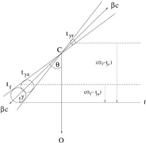
Figure 9: Assumed geometry of the jet. C is the core of the system, and the observer is in direction O. The plasmon centres move outwards at speed $\beta c$ and the jet axis is aligned at angle $i$ to the line of sight. We use the co-ordinate $y$ as a dimensionless local measure of the distance from the front surface to any plane within a given plasmon. Light from position $y$ within a plasmon leaves that plasmon in the approaching jet at time $t_{\rm{ya}}$ in order to reach plane $f$ at time $t_{\rm{f}}$. Light from position $y$ within the corresponding plasmon in the receding jet leaves at an earlier time $t_{\rm{yr}}$ in order to reach $f$ at this same time. All light leaving $f$ at time $t_{\rm{f}}$ will obviously be received at the same time by the observer.

Our toy model is shown in Figure 9; our analysis follows that of Blundell & Alexander (1994) who considered analogous effects in the evolution of the lobes of radio galaxies. We consider light setting off from the closest point of the first plasmon to the observer, and determine what time the light would have left other parts of that plasmon, and other plasmons, in order to reach plane $f$ at the same time. All light leaving plane $f$ (perpendicular to the line of sight) at a given instant clearly reaches the observer simultaneously. The refractive index of the plasmons is taken to be 1 (in reality, it will be greater than 1, and this will make the light travel-time effects even more significant). We assume a tangled field, so that the magnetic flux density falls off as $B\propto R^{-1}$ (as described in § 7.2.1). Given the magnetic field at any one time, and having calculated the time the light set off from a plane within a plasmon, and knowing the time at which the plasmon was ejected, then assuming constant uniform expansion of the plasmons, the size of a plasmon at any given time, and therefore its magnetic field can be determined. Dividing each plasmon up into slices perpendicular to the line of sight, from which light sets off progressively earlier, we derive the field in each slice at the time at which light leaves that slice. We can then calculate the emissivity of each slice, assuming the plasmons to be homogeneously filled with energetic particles. We then integrate over the entire plasmon to find the flux density expected at any particular frequency, having corrected for Doppler boosting and relativistic time-dilation effects.

To model the emissivity of each slice, rather than take the full expression for the synchrotron emissivity, we assume that each electron radiates at a single frequency, determined by its Lorentz factor and the ambient magnetic field (Equation 9). In order to model the opacity, we put in an absorption coefficient (derived either for synchrotron self-absorption, or for free-free absorption, as in Rybicki & Lightman (1979)). We calculate the location of the $\tau=1$ surface within each plasmon at each frequency, and assume we see no emission from beyond that surface. Emission from the near side of the $\tau=1$ surface is taken to be synchrotron emission from a power-law distribution of electrons with electron index $p=2.2$. This produces a turned-over spectrum as we observe. We then observe how the spectrum evolves with time.

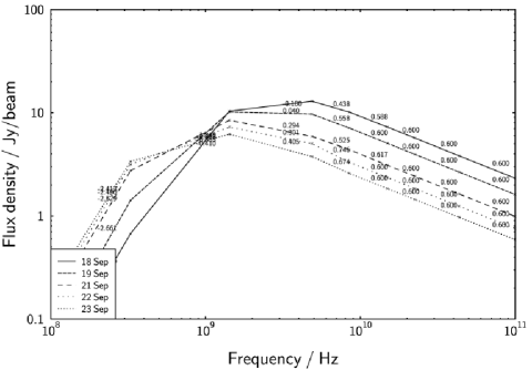
Figure 10: Model spectra for 2001 September 18, 19, 21, 22, and 23, to be compared with Figure 6. Spectral indices between each sampled frequency point are given. The model takes into account light travel-time and opacity effects for a series of jet knots, with adiabatic expansion of a series of ejected plasmons governing the spectral evolution. As shown above, it does not include any flat-spectrum core component.

Plots of spectra generated are given in Figure 10. The full theory will be explored in more detail in a companion paper (Miller-Jones et al. in prep.). For now, we note that such a model produces the qualitative features of spectra similar to those observed, in that it produces a turnover moving to lower frequencies with time and a steepening of the spectrum at frequencies just above the turnover to a terminal value of the spectral index which corresponds to the underlying electron energy index. An important success of this model is that the timescales for the movement of the turnover and for the steepening of the high-frequency spectrum match those observed.

However, where this model falls short is that it does not predict a spectrum flatter than $\nu^{-0.6}$ all the way up to the highest observing frequencies. However, this model only includes jet knots which evolve as described above: it takes no account of any flat-spectrum core component. We note that invoking the addition of a core with a canonical $\nu^{-0.1}$ spectrum whose intensity decreases with time might sufficiently flatten the predicted high-frequency spectrum at early epochs. Such a core component was postulated in § 6.4.4 (see also Figure 5) and was present in this outburst, as we now describe. In § 6.5, we found that the observed VLBA knots appeared to have been ejected $2.5\pm 0.5$ days after the integrated radio flux density began to rise. This would be consistent with a scenario in which a flat-spectrum core component as postulated above dominated the flux density initially, but faded over time. After the ejection of the steep-spectrum radio plasmons, their flux density would later come to dominate the observed flux density, especially at lower frequencies.

10 Comparison to radio galaxies

We now make a brief comparison between the magnetic field and energy budget in this microquasar flare and those parameters in quasars: scaled-up, longer-lived versions of Cygnus X-3.

10.1 Magnetic Field

M 87 is a radio galaxy at a distance of 16 Mpc for which there are good constraints on the magnetic field at different distances from the core, which has a central black hole of mass $3.2\pm 0.9\times 10^{9}$ $M_{\odot}$(Macchetto et al., 1997). Reynolds et al. (1996) derived limits to the magnetic field in the jet of M 87 of $0.01<B<0.2$ G at an angular separation of 0.1 mas from the core, approximately 1800 AU, or 40 gravitational radii ($r_{\rm{G}}$) from the central engine. Heinz & Begelman (1997) derived a magnetic field of $5<B<49\,\mu$G at several kpc ($\sim 10^{6}-10^{7}r_{\rm{G}}$) from the core. Standard equipartition arguments give $300<B<600\,\mu$G at that distance (e.g. Meisenheimer et al., 1996).

Cygnus X-3 is thought to contain either a neutron star or a black hole of a few solar masses (e.g. van den Heuvel & de Loore, 1973; Schmutz et al., 1996; Ergma & Yungelson, 1998; Stark & Saia, 2003): a factor of $10^{8}-10^{9}$ times smaller than the black hole in M 87. Assuming that the compact object in Cygnus X-3 has a mass of a few solar masses, its gravitational radius is of order 10 km. Observing with a few mas resolution probes the source at $10^{8}-10^{9}\,r_{\rm{G}}$. According to Heinz (2002), magnetic fields in the inner jet and disk should scale as $M^{-1/2}$ where $M$ is the black hole mass. Comparing the magnetic fields in the inner jets of M 87 and Cygnus X-3  this predicts the field in the inner jet (tens of gravitational radii from the compact object) of Cygnus X-3 to be of order $10^{3}$ G. This is a factor of $10^{4}$ higher than that which we observe further out at $\sim 10^{8}\,r_{\rm{G}}$. Let $R$ be the jet cross-section and $r$ the distance from the core measured along the jet axis. Taking a jet model in which the cross-section scales as $R\propto r^{\delta}$, and invoking flux-freezing and a tangled magnetic field, such that $B\propto R^{-1}$, we find that $B\propto r^{-\delta}$. Putting in the values we have for $B$ and $r$, we find that $0.50<\delta<0.83$. This limit may be compared with theoretical limits quoted by Heinz & Sunyaev (2002). They found that

$$R =R_{0}(r/r_{0})^{\beta},\qquad 0<\beta<1$$ (29)

$$n =n_{0}(r/r_{0})^{-\lambda},\qquad 2\beta\leq\lambda\leq 3\beta$$ (30)

$$B =B_{0}(r/r_{0})^{-\delta},\qquad 1/2\lambda\leq\delta\leq\lambda$$ (31)

where they defined $r$ as the distance from the black hole, $r_{0}$ as the distance at which the jet is injected (taken as 10 $r_{\rm G}$), $R$ as the jet cross-section and $n$ as the particle number density. They did however point out that this assumes self-similarity. It would thus be expected to hold in the inner jet, but not necessarily further out where the jet behaviour may be dominated by interactions with its environment. The case $\beta=1$ corresponds to a jet with constant opening angle. A jet composed of discrete ejections has $\lambda\sim 3\beta$, whereas a continuous jet would satisfy $\lambda\sim 2\beta$. A value $\delta=2/3\lambda$ is predicted for a completely tangled magnetic field. From the VLBA observations in Section 5, we observed a jet which seems to be composed of discrete ejections, and we have assumed a tangled field. Thus we would expect $\delta=2\beta$. Our derived limits on the value of the index $\delta$ then imply $0.25<\beta<0.41$. Since the VLBA images did not have sufficient transverse resolution to monitor the jet opening angle, and since they showed a series of discrete knots in the jet, it is not possible to verify accurately any variation in the opening angle from the observations.

We note, however, that although we expect similar physics to apply in the inner, jet-producing regions of AGN and microquasars, the environments of the two types of system are different. According to Heinz (2002), in dynamical terms, microquasar jets are located in relatively low-pressure, low-density environments. Where we observe the radio jets (i.e. as they interact with their environments), the characteristics of the environment will affect the kinematics of the jet, and a simple scaling between the two types of system is not expected.

Heinz & Begelman (1997) found that the magnetic field in the M 87 jet at a distance of several kpc from the core should be a factor $\sim 1.5-5$ times lower than the equipartition value. We found the Cygnus X-3 outer jet to be out of equipartition (modulo the uncertainties in this calculation) by a similar factor of a few (§ 8.4).

10.2 Energetics

The typical energy thought to be stored in the lobes of a radio galaxy such as Cygnus A is estimated to be of order $10^{59}$ erg (Kembhavi & Narlikar, 1999, chapter 9), and the typical kinetic jet power of order $10^{42}-10^{43}$ erg s^-1 (Reynolds et al., 1996). From the results of September 18, it is possible to deduce the minimum energy present in the outburst, using the $\gamma_{\rm{max}}$ and $\gamma_{\rm{min}}$ corresponding to the highest and lowest observed frequencies on that date. This gives a lower limit of $8.5\times 10^{42}$ erg for the energy released following this flare. We do not believe, however, that we have fully sampled the range of Lorentz factors present in the jet, so this should be taken as a lower limit, and fuller sampling would be required in order to make a complete comparison with AGN.

11 Conclusions

We have presented time-sequenced milliarcsecond-resolution observations at three different frequencies of a major outburst of Cygnus X-3, accompanied by simultaneous quasi-daily monitoring of the (unresolved) flux density of the source, with unprecedented spectral coverage of a large flare, ranging over three decades in frequency. The proper motions of individual plasmons have been directly tracked for the first time, and the expansion of those plasmons has been directly measured.

One main result is to securely determine the presence of a two-sided jet in Cygnus X-3 on milliarcsecond scales following a major flare. The southern jet appears to be approaching and the northern counterjet appears to be receding from us, being substantially de-boosted. We derived a jet speed of $\beta\sim 0.63$. The jet appears to be precessing with a period of order 5.3 days, significantly shorter than that derived by Mioduszewski et al. (2001) for the 1997 flare. It appears that the milliarcsecond-scale jet is not ejected immediately on the rise of the integrated flux density, but $\sim 2.5$ days after this, a point which we explore in a forthcoming paper (Miller-Jones et al. in prep.).

We believe that it is possible that the intrinsic characteristics of Cygnus X-3 in the outbursts of, for example, 1997 and 2001, may have been different. It is not clear that all outbursts of such sources follow the same patterns. Certainly the flux densities and fading times are not the same for different events, as outlined above. This variable, almost whimsical, nature of the source needs to be clarified. Certain parameters would not be expected to change (e.g. after accounting for precession, the inclination angle of the jet axis to the line of sight might be expected to be constant). Identical spectral, temporal, and uv-coverage of different events with similar radio lightcurves might help to determine whether the jet parameters are indeed constant for different flares.

Observations of the integrated flux density of the source showed an evolving spectrum similar to that seen in previous outbursts of Cygnus X-3. The high-frequency spectrum at frequency $\nu$ took the form $\nu^{-\alpha}$, where $\alpha$ steepened from $\sim 0.4$ to $\sim 0.6$ and the spectral index then remained at this latter terminal value. We contend that the spectral evolution is the result of light travel-time effects in plasmons which were initially optically thick, but which became optically thin as they expanded. Such a model can produce spectral evolution over timescales similar to those observed. Confirmation that opacity effects are important came from the integrated spectrum between 1.4 GHz and 74 MHz: this showed a turnover moving to lower frequencies with time, caused by the decreasing opacity (probably caused by either synchrotron self-absorption, free-free absorption or a low-energy cutoff in the electron spectrum). The presence of an additional flat-spectrum core component which was responsible for the initial rise of the flare but which then faded with time was also postulated.

We derived an upper limit to the magnetic field in the plasmons of $0.15\pm 0.06$ G, consistent with previous estimates for similar systems. We also placed lower limits on the minimum and maximum observed Lorentz factors of the emitting electrons, of $\gamma=58$ and $\gamma=321$.

Despite the unique nature of this system, Cygnus X-3 does share many of the characteristics of other, better understood microquasars. Owing to its position within the Galaxy and the associated difficulties in imaging the system, Cygnus X-3 still remains somewhat of an enigma. Studying it can, however, enhance our understanding of the effects which we believe must play a part in the observed emission from microquasars. Light travel-time effects are unavoidable in systems of this size evolving on similar timescales.

Table 1: Cygnus X-3 VLA Flux Densities

Date (UT)	JD-2450000	Observing Frequency (GHz)	Flux Density (Jy)
2001 September 09	$2161.73955\pm 0.00050$	04.860	$0.0209\pm 0.0007$
	$2161.73356\pm 0.00046$	08.460	0$0.0312\pm 0.0005$
	$2161.73212\pm 0.00075$	14.940	0$0.0424\pm 0.0020$
	$2161.72419\pm 0.00127$	22.460	0$0.0387\pm 0.0030$
	$2161.71748\pm 0.00139$	43.340	0$0.0472\pm 0.0038$
2001 September 18	$2170.57112\pm 0.00168$	01.385	0$8.56\pm 0.17$
	$2170.57112\pm 0.00168$	01.465	0$9.16\pm 0.18$
	$2170.57570\pm 0.00093$	04.860	$13.41\pm 0.27$
	$2170.57778\pm 0.00093$	08.460	$11.85\pm 0.12$
	$2170.59215\pm 0.00091$	14.940	0$9.04\pm 0.43$
	$2170.58810\pm 0.00197$	22.460	0$7.44\pm 0.57$
	$2170.58351\pm 0.00168$	43.340	0$5.99\pm 0.46$
2001 September 19	$2171.45749\pm 0.00050$	01.385	$14.25\pm 0.28$
	$2171.45749\pm 0.00050$	01.465	$14.31\pm 0.29$
	$2171.45660\pm 0.00058$	04.860	$13.43\pm 0.27$
	$2171.46615\pm 0.00052$	08.460	$10.54\pm 0.11$
	$2171.48380\pm 0.00058$	14.940	0$8.22\pm 0.39$
	$2171.48079\pm 0.00127$	22.460	0$6.70\pm 0.51$
	$2171.47454\pm 0.00127$	43.340	0$4.62\pm 0.37$
2001 September 21	$2173.63970\pm 0.00058$	01.385	0$7.98\pm 0.16$
	$2173.63970\pm 0.00058$	01.465	0$7.86\pm 0.16$
	$2173.64092\pm 0.00041$	04.860	0$4.83\pm 0.10$
	$2173.65000\pm 0.00046$	08.460	0$3.54\pm 0.04$
	$2173.66476\pm 0.00041$	14.940	0$2.37\pm 0.11$
	$2173.66119\pm 0.00050$	22.460	0$1.79\pm 0.14$
	$2173.65567\pm 0.00046$	43.340	0$1.22\pm 0.15$
2001 September 22	$2174.52118\pm 0.01806$	00.3275	0$6.161\pm 1.4$00
	$2174.50232\pm 0.00058$	01.385	0$5.640\pm 0.113$
	$2174.50232\pm 0.00058$	01.465	0$5.377\pm 0.108$
	$2174.52558\pm 0.01782$	04.860	0$2.968\pm 0.059$
	$2174.53115\pm 0.01587$	08.460	0$2.126\pm 0.021$
	$2174.53671\pm 0.00091$	14.940	0$1.465\pm 0.070$
	$2174.52646\pm 0.00108$	43.340	0$0.688\pm 0.055$
2001 September 23	$2175.70995\pm 0.01053$	00.0738	$<2.7$
	$2175.70723\pm 0.01048$	00.3275	0$4.061\pm 1.4$00
	$2175.69601\pm 0.00052$	01.385	0$2.919\pm 0.058$
	$2175.69601\pm 0.00052$	01.465	0$2.834\pm 0.057$
	$2175.70139\pm 0.00046$	04.860	0$1.425\pm 0.029$
	$2175.70642\pm 0.00041$	08.460	0$0.990\pm 0.010$
	$2175.71570\pm 0.00062$	14.940	0$0.641\pm 0.031$
	$2175.71250\pm 0.00058$	22.460	0$0.492\pm 0.038$
	$2175.71078\pm 0.00091$	43.340	0$0.315\pm 0.030$
2001 September 24	$2176.69213\pm 0.01563$	00.0738	$<4.5$
	$2176.68918\pm 0.01557$	00.3275	$7.001\pm 1.4$00
	$2176.69371\pm 0.02157$	01.385	$1.893\pm 0.038$
	$2176.69371\pm 0.02157$	01.465	0$1.842\pm 0.037$
	$2176.69618\pm 0.01794$	04.860	0$0.895\pm 0.018$
	$2176.69699\pm 0.03117$	08.460	0$0.638\pm 0.006$
	$2176.69884\pm 0.00058$	14.940	0$0.470\pm 0.022$
	$2176.69220\pm 0.00065$	22.460	0$0.392\pm 0.030$
	$2176.69041\pm 0.00091$	43.340	0$0.314\pm 0.016$

Note. — The error bars given were derived as described in 3.3

Table 2: Cygnus X-3 OVRO Millimeter Array Flux Densities at 99.48 GHz

Date (UT)	JD-2450000	Flux Density (Jy)
2001 Sep 20	$2172.6930\pm 0.0597$	$1.206\pm 0.005$
2001 Sep 21	$2173.6242\pm 0.0167$	$0.942\pm 0.007$
2001 Sep 22	$2174.8232\pm 0.0170$	$0.363\pm 0.010$
2001 Sep 23	$2175.6892\pm 0.0205$	$0.216\pm 0.005$
2001 Sep 26	$2178.5559\pm 0.0275$	$0.121\pm 0.004$

Note. — The uncertainties quoted in the flux density are those due to thermal noise.

Table 3: VLBA image parameters

Date (UT)	JD-2450000	$\nu$ (GHz)	Beam (mas $\times$ mas)	Beam P.A.	Scattering Disk Size (mas)	r.m.s. (mJy bm-1)
2001 Sep 18	$2170.78779\pm 0.17781$	22.233	0$8.59\times 3.48$0	$-59.4$	$\phantom{0}0.69\pm 0.22$	019.70
	$2170.76849\pm 0.18423$	04.995	$13.71\times 12.92$	$+16.7$	$15.54\pm 2.42$	013.80
2001 Sep 19	$2171.61065\pm 0.20914$	22.233	0$8.30\times 4.00$0	$-29.1$	$\phantom{0}0.69\pm 0.22$	009.68
	$2171.59074\pm 0.20183$	15.365	$16.19\times 8.76$0	$-19.8$	$\phantom{0}1.48\pm 0.42$	126.40
	$2171.59149\pm 0.21542$	04.995	$15.65\times 13.58$	$-63.9$	$15.54\pm 2.42$	006.38
2001 Sep 20	$2172.75584\pm 0.20548$	22.233	0$5.88\times 3.77$0	$-59.2$	$\phantom{0}0.69\pm 0.22$	006.52
	$2172.72633\pm 0.18880$	15.365	0$9.39\times 8.91$0	$+19.2$	$\phantom{0}1.48\pm 0.42$	042.00
	$2172.71344\pm 0.18880$	04.995	$14.54\times 13.45$	$-85.8$	$15.54\pm 2.42$	017.90
2001 Sep 21	$2173.65190\pm 0.26304$	15.365	$13.31\times 9.00$0	$-14.4$	$\phantom{0}1.48\pm 0.42$	021.00
	$2173.63907\pm 0.26305$	04.995	$11.85\times 10.60$	$+61.4$	$15.54\pm 2.42$	007.49

Table 4: Fitted Gaussian FWHM sizes of the 22 GHz VLBA knots

Date	Component	Fitted FWHM (mas)	Major Axis (mas)	Minor Axis (mas)	P.A.
2001 Sep 18	Single component	$7.88\pm 0.51$	$7.23\pm 0.17$	$2.65\pm 0.34$	$167.5\pm 2.0$
2001 Sep 19	North	$11.98\pm 0.15$	$11.00\pm 0.14$	$4.03\pm 0.09$	$168.1\pm 0.7$
2001 Sep 19	South	$13.36\pm 0.21$	$10.93\pm 0.23$	$5.04\pm 0.12$	$157.5\pm 1.2$
2001 Sep 20	North	$14.37\pm 0.54$	$10.58\pm 0.39$	$6.02\pm 0.39$	$26.5\pm 94.3$
2001 Sep 20	South	$16.92\pm 0.88$	$13.89\pm 0.71$	$6.36\pm 0.58$	$25.0\pm 95.8$

Note. — Deconvolved sizes and errors were derived using the AIPS task JMFIT

Table 5: Results of fitting the 22 GHz VLBA image of September 20 with the Hjellming & Johnston precessing jet model

Core R.A.	Core Dec.	$s_{\rm rot}$	Parameter	Mean	Standard Deviation	Maximum	Minimum
20 32 25.77335	+40 57 27.9650	-1	$\phi$	168.8	91.1	345.9	3.3
			$\psi$	2.4	1.2	5.8	0.4
			$i$	10.5	4.2	18.8	2.5
			$\chi$	98.9	2.9	106.2	93.4
			$\beta$	0.63	0.09	0.80	0.47
			$P$ (days)	5.34	0.67	7.15	3.73
			$d$ (kpc)	10.8	2.6	14.8	5.6
			$t_{\rm view}$ (days)	7.44	0.54	8.43	6.08
20 32 25.77335	+40 57 27.9650	+1	$\phi$	136.1	97.7	330.2	2.1
			$\psi$	2.2	0.9	4.3	0.8
			$i$	169.6	3.8	175.6	161.3
			$\chi$	278.1	2.8	283.6	273.6
			$\beta$	0.60	0.08	0.77	0.49
			$P$ (days)	5.49	0.46	7.06	4.81
			$d$ (kpc)	10.0	2.1	13.0	6.2
			$t_{\rm view}$ (days)	7.53	0.52	8.42	6.61

Note. — All angles ($\phi$, $\psi$, $i$, and $\chi$) are measured in degrees

References

- Aller & Dent (1972) Aller, H.D., & Dent, W.A. 1972, Nature Physical Science, 239, 121
- Atoyan & Aharonian (1997) Atoyan, A.M., & Aharonian, F.A. 1997, ApJ, 490, L149
- Atoyan & Aharonian (1999) Atoyan, A.M., & Aharonian, F.A. 1999, MNRAS, 302, 253
- Blundell & Alexander (1994) Blundell, K.M., & Alexander, P. 1994, MNRAS, 267, 241
- Butler (2001) Butler, B.J. 2001, VLA Scientific Memo 176
- Butler (2002) Butler, B.J. 2002, VLA Test Memo 232
- Choudhury et al. (2002) Choudhury, M., Rao, A.R., Vadawale, S.V., Ishwara-Chandra, C.H., & Jain, A.K. 2002, A&A, 383, 35
- Clark (1973) Clark, B.G. 1973, VLA Computer Memorandum 105
- Dickey (1983) Dickey, J.M. 1983, ApJ, 273, L71
- Ergma & Yungelson (1998) Ergma, E., & Yungelson, L.R. 1998, A&A, 333, 151
- Fender et al. (1997) Fender, R.P., Bell Burnell, S.J., Waltman, E.B., Pooley, G.G., Ghigo, F.D., & Foster, R.S. 1997, MNRAS, 288, 849
- Fomalont, Geldzahler & Bradshaw (2001) Fomalont, E.B., Geldzahler, B.J., & Bradshaw, C.F. 2001, ApJ, 558, 283
- Fomalont & Perley (1999) Fomalont, E.B., & Perley, R.A. 1999, in ASP Conf. Ser. 180, Synthesis Imaging in Radio Astronomy II, ed. Taylor, G.B., Carilli, C.L., & Perley, R.A. (San Francisco: ASP), 97
- Geldzahler et al. (1983) Geldzahler, B.J. et al. 1983, ApJ, 273, L65
- Giacconi et al. (1967) Giacconi, R., Gorenstein, P., Gursky, H., & Waters, J.R. 1967, ApJ, 148, L119
- Gregory et al. (1972a) Gregory, P.C. et al. 1972a, Nature Physical Science, 239, 114
- Gregory et al. (1972b) Gregory, P.C., Kronberg, P.P., Seaquist, E.R., Hughes, V.A., Woodsworth, A., Viner, M.R., & Retallack, D. 1972b, Nature Physical Science, 239, 440
- Gregory & Seaquist (1974) Gregory, P.C., & Seaquist, E.R. 1974, ApJ, 194, 715
- Heinz (2002) Heinz, S. 2002, A&A, 388, L40
- Heinz & Sunyaev (2002) Heinz, S., & Sunyaev, R.A. 2002, in ESO Astrophysics Symp., Lighthouses of the Universe: The Most Luminous Celestial Objects and Their Use for Cosmology, eds. M. Gilfanov, R. Sunyaev, & E. Churazov (Berlin: Springer), 453
- Heinz & Begelman (1997) Heinz, S., & Begelman, M.C. 1997, ApJ, 490, 653
- Hjellming & Balick (1972) Hjellming, R.M., & Balick, B. 1972, Nature Physical Science, 239, 135
- Hjellming et al. (1974) Hjellming, R.M., Brown, R.L., & Blankenship, L.C. 1974, ApJ, 194, L13
- Hjellming & Johnston (1981) Hjellming, R.M., & Johnston, K.J. 1981, ApJ, 246, L141
- Hjellming & Johnston (1988) Hjellming, R.M., & Johnston, K.J. 1988, ApJ, 328, 600
- Kellermann (1966) Kellermann, K.I. 1966, Aust. J. Phys., 19, 195
- Kembhavi & Narlikar (1999) Kembhavi, A.K., & Narlikar, J.V., 1999, Quasars and Active Galactic Nuclei, (Cambridge: Cambridge University Press)
- Koch-Miramond et al. (2002) Koch-Miramond, L., Ábráham, P., Fuchs, Y., Bonnet-Bidaud, J.-M., & Claret A. 2002, A&A, 396, 877
- Landau & Lifshitz (1963) Landau, L.D., & Lifshitz, E.M. 1963, Course of Theoretical Physics, Vol. 8: Electrodynamics of continuous media (2nd ed.; Oxford: Pergamon)
- Longair (1994) Longair, M.S. 1994, High energy Astrophysics, Vol. 2: Stars, the Galaxy and the interstellar medium(2nd ed.; Cambridge: CUP)
- Macchetto et al. (1997) Macchetto, F., Marconi, A., Axon, D.J., Capetti, A., Sparks, W., & Crane, P. 1997, ApJ, 489, 579
- Marscher (1987) Marscher, A.P. 1987, in Superluminal radio sources, eds. J.A. Zensus & T.J. Pearson, (Cambridge: Cambridge University Press), 280
- Marscher (1983) Marscher, A.P. 1983, ApJ, 264, 296
- Marsh et al. (1974) Marsh, K.A., Purton, C.R., & Feldman, P.A. 1974, ApJ, 192, 697
- Martí et al. (1992) Martí, J., Paredes, J.M., & Estalella, R. 1992, A&A, 258, 309
- Martí et al. (2001) Martí, J., Paredes, J.M., & Peracaula, M. 2001, A&A, 375, 476
- McCollough et al. (1999) McCollough, M.L. et al. 1999, ApJ, 517, 951
- Meisenheimer et al. (1996) Meisenheimer, K., Rser, H.-J., & Schltelburg, M. 1996, A&A, 307, 61