Particle acceleration in cooling flow clusters of galaxies: the case of Abell 2626

It has recently been proposed a theoretical model which accounts for the origin of radio mini–halos observed in some cooling flow clusters as related to electron re–acceleration by MHD turbulence (Gitti, Brunetti & Setti 2002). The MHD turbulence is assumed to be frozen into the flow of the thermal ICM and thus amplified in the cooling flow region. Here we present the application of this model to a new mini–halo candidate, the cluster A2626, and compare the results with those obtained for the mini–halo in the Perseus cluster. We present VLA data at 330 MHz and 1.5 GHz of the diffuse radio emission observed in A2626, and we show that its main properties can be explained by the model. We find that the power necessary for the re–acceleration of the relic electron population is only a factor $\sim 0.7$ % of the maximum power that can be extracted by the cooling flow (as estimated on the basis of the standard model). We also discuss the observational properties of known mini–halos in connection with those of host clusters, showing that the radio power of mini–halos increases with the maximum power of cooling flows. This trend is expected in the framework of the model. Possible effects of new Chandra and XMM–Newton estimates of $\dot{M}$ on this trend are considered: we conclude that even if earlier derived cooling rates were overestimated, cooling flow powers are still well above the radio powers emitted by mini–halos.

1 Introduction

A number of clusters of galaxies show extended synchrotron emission not directly associated with the galaxies but rather diffused into the intra–cluster medium (ICM). These radio sources have been classified in three classes: cluster–wide halos, relics and mini–halos (Feretti & Giovannini 1996). Both cluster–wide halos and relics have low surface brightness, large size ($\sim$ 1 Mpc) and steep spectrum, but the former are located at the cluster centers and show low or negligible polarized emission, while the latter are located at the cluster peripheries and are highly polarized. They have been found in clusters which show significant evidence for an ongoing merger (e.g., Edge, Stewart & Fabian 1992; Giovannini & Feretti 2002). It was proposed that recent cluster mergers may play an important role in the re–acceleration of the radio–emitting relativistic particles, thus providing the energy to these extended sources (e.g., Schlickeiser, Sievers & Thiemann, 1987; Tribble 1993; Brunetti et al. 2001). The merger picture is consistent with the occurrence of large–scale radio halos in clusters without a cooling flow, since the major merger event is expected to disrupt a cooling flow (e.g., Sarazin 2002 and references therein).

In spite of the observed anti–correlation between the presence of cooling flows and extended radio emission in clusters of galaxies, there are several cooling flow clusters where the relativistic particles can be traced out quite far from the central galaxy, forming what is called a “mini–halo” (e.g. Perseus: Burns et al. 1992; Abell 2390: Bacchi et al. 2003). Mini–halos are diffuse steep–spectrum radio sources, extended on a moderate scale (up to $\sim 500$ kpc), surrounding a dominant radio galaxy at the center of cooling flow clusters. Until recently, because of the presence of the central radio galaxy, these sources have been considered of different nature from that of extended halos and relics, and the problem of their origin has never been investigated in detail.

Mini–halos do not appear as extended lobes maintained by an Active Galactic Nucleus (AGN), as in classical radio galaxies (Giovannini & Feretti 2002), therefore their radio emission is indicative of the presence of diffuse relativistic particles and magnetic fields in the ICM. Rizza et al.(2000) presented three-dimensional numerical simulations of perturbed jet propagating through a cooling flow atmosphere in order to study the interaction between the radio plasma and the hot ICM in cooling flow clusters containing steep–spectrum radio sources. The evolution and spectrum of relativistic particles, however, is not considered in these simulations. The point is that the radiative lifetime of the radio–emitting electrons injected at a given time in the strong magnetic fields present in cooling flow regions is of the order of $\sim 10^{7}$ - $10^{8}$ yr, much shorter than the transport time necessary to cover $\sim$ hundred kpc scales, so that the diffuse radio emission from mini–halos may suggest the presence of re–accelerated electrons.

More specifically, Gitti, Brunetti & Setti (2002, hereafter GBS) suggested that the diffuse synchrotron emission from radio mini–halos is due to a relic population of relativistic electrons re–accelerated by MHD turbulence via Fermi–like processes, with the necessary energetics supplied by the cooling flow.

Alternatively, Pfrommer & Enßlin (2003) in a very recent paper discussed the possibility that the radiating electrons in radio mini–halos are of secondary origin and thus injected during proton-proton collision in the ICM.

The main aim of the present work is the application of GBS’s model to a new mini-halo candidate, A2626 ($z=0.0604$, Rizza et al. 2000), and the discussion of the observational properties of the population of radio mini–halos so far discovered.

In Sect. 2 we briefly review GBS’s model and its application to the Perseus cluster. In Sect. 3 we consider the radio source observed in A2626: first, we present VLA data analysis and discuss the possibility that this source belongs to the mini–halo class, then we apply GBS’s model to this cluster and discuss the results. In Sect. 4 we present the observational properties of other radio mini–halo candidates in relation to those of host clusters and discuss them in the framework of GBS’s model.

For consistency with GBS, a Hubble constant $\mbox{H}_{0}=50\mbox{ km s}^{-1}\mbox{ Mpc}^{-1}$ is assumed in this paper, therefore at the distance of A2626 $1^{\prime}$ corresponds to $\sim$ 95 kpc. The radio spectral index $\alpha$ is defined such as $S_{\nu}\propto\nu^{-\alpha}$ and, where not specified, all the formulae are in cgs system.

2 Electron re–acceleration in cooling flows

The radiative lifetime of an ensemble of relativistic electrons losing energy by synchrotron emission and inverse Compton (IC) scattering off the CMB photons is given by:

$$\tau_{\rm sin+IC}\simeq\frac{2.5\times 10^{13}}{\left[\left(B/\mu\mbox{G}\right)^{2}+\left(B_{\rm\tiny CMB}/\mu\mbox{G}\right)^{2}\right]\,\gamma}\;\;\;\mbox{yr}$$ (1)

where $B$ is the magnetic field intensity, $\gamma$ is the Lorentz factor and $B_{\rm\tiny CMB}=3.18(1+z)^{2}\mu$G is the magnetic field equivalent to the CMB in terms of electron radiative losses. In a cooling flow region the compression of the thermal ICM is expected to produce a significant increase of the strength of the frozen–in intra–cluster magnetic field and consequently of the electron radiative losses. Therefore, in the absence of a re–acceleration or continuous injection mechanisms, relativistic electrons injected at a given time in these strong fields (of order of 10 - 20 $\mu$G, e.g., Ge & Owen 1993; Carilli & Taylor 2002) should already have lost most of their energy and the radio emission would not be observable for more than $\sim 10^{7}$ - $10^{8}$ yr. This short lifetime contrasts with the diffuse radio emission observed in mini–halos.

In order to evaluate the radiative losses in the cooling flow region at any distance from the cluster center it is necessary to parameterize the radial dependence of the field strength, which depends on the compression of the thermal gas in the cooling region (i.e., on $n(r/r_{\rm c})$, $r_{\rm c}$ being the cooling radius). However, it should be born in mind that while the X–ray brightness and low resolution spectra are generally in agreement with the standard cooling flow model, recent observations with the Reflection Grating Spectrometer (RGS) on board XMM–Newton do not show evidence for gas cooling at temperatures lower than 1-2 keV (e.g., Peterson et al. 2003) as expected in the standard picture. In addition, both Chandra and XMM–Newton results indicate that the mass deposition rates in cooling flows have been previously overestimated by a factor 5-10 (e.g., Fabian & Allen 2003). It is worth noticing that the new rates lead to mass values not too different from the large masses of cold gas derived from the studies of the CO emission line detected in a number of cooling flow cluster candidates (Edge 2001; Salomé & Combes 2003). These findings, although not inconsistent with the idea that the gas cools down and is thus compressed towards the central region, point to a more complex situation than that described by the standard cooling flow model. Unfortunately, no successful model in alternative to the standard model has been proposed yet and, therefore, we will evaluate the radial behaviour of the physical quantities in the ICM by making use of the standard – single phase – cooling flow model.

In the framework of this model, the intensity of the frozen–in magnetic field increases as $B\propto r^{-2}$ for radial compression (Soker & Sarazin 1990) or $B\propto r^{-0.8}$ for isotropic compression (Tribble 1993).

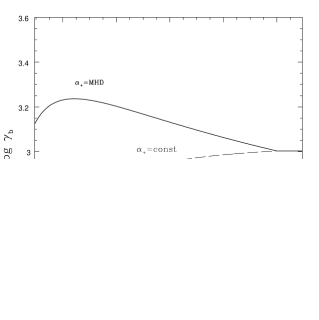
Figure 1: Evolution of $\gamma_{\rm b}$ inside the cooling flow region for two different cases of re–acceleration: $\bullet\,\alpha_{+}$ given by Fermi–like processes related to the MHD turbulence in the cooling flow (bold line; Eq. 4 for typical values of the parameters), and $\bullet\,\alpha_{+}$=constant (dashed line).

The time evolution of the energy of a relativistic electron is determined by the competing processes of losses and re–accelerations (both related to the magnetic field) :

$$\dot{\gamma}(x)=-\beta(x)\gamma^{2}(x)+\alpha_{+}(x)\gamma(x)-\chi(x)$$ (2)

where $x=r/r_{\rm c}$, $\beta=\gamma^{-1}/\tau_{\rm sin+IC}$ is the coefficient of synchrotron and IC losses, $\alpha_{+}$ is the re–acceleration coefficient, which mimics the systematic rate of average energy increase resulting from stochastic acceleration (see GBS), and $\chi$ the Coulomb loss term. GBS developed a model for radio mini–halos consisting in the re–acceleration of relativistic electrons by MHD turbulence via Fermi–like processes. The MHD turbulence is assumed to be frozen into the flow of the thermal ICM and is thus amplified due to the compression of the turbulent coherence length scale and the amplification of the magnetic field in the cooling flow region. In the present paper, we consider a coefficient for systematic re–acceleration given by (Melrose 1980):

$$\alpha_{+}(x)\approx(\pi/c)\,v_{\rm A}^{2}(x)\,l^{-1}(x)\,[\delta B(x)/B(x)]^{2}$$ (3)

where $v_{\rm A}=\sqrt{B^{2}/4\pi\rho}$ is the Alfvén velocity and $l$ is the characteristic MHD turbulence scale. For simplicity we assume a fully developed turbulence with $\delta B(x)/B(x)\sim{\rm const}$. The energy at which the losses are balanced by the re–acceleration, $\gamma_{\rm b}$, is obtained by Eq. 2 and, since Coulomb losses are nearly negligible at such electron energies, it is $\gamma_{b}\approx\alpha_{+}/\beta$. The evolution of $\gamma_{\rm b}$ in the cooling flow region can be written in terms of the two free parameters $B_{\rm c}=B(r_{\rm c})$ and $l_{\rm c}=l(r_{\rm c})$, resulting in (isotropic compression of the field is assumed, as motivated in Sect. 3.2):

$$\gamma_{\rm b}(x)=\frac{1.23\times 10^{4}\,\left(\frac{B_{\rm c}}{1\mu\mbox{\tiny G}}\right)^{2}\,x^{-0.8}(\delta B_{\rm c}/B_{\rm c})^{2}}{\left(\frac{l_{\rm c}}{100\mbox{ \tiny pc}}\right)\left(\frac{n_{\rm c}}{10^{-3}\mbox{ \tiny cm}^{-3}}\right)\left[\left(\frac{B_{\rm c}}{1\mu\mbox{\tiny G}}\right)^{2}x^{-1.6}+10\right]}$$ (4)

where $n_{\rm c}$ is the proton number density at $r_{\rm c}$, and we used the relations $l(x)=l_{\rm c}\,x^{0.4}$ and $n(x)=n_{\rm c}\,x^{-1.2}$ (see GBS). The behaviour of $\gamma_{\rm b}(x)$ is shown in Fig. 1: being able to make $\gamma_{\rm b}(x)$ weakly increasing inside the cooling flow region, the re–acceleration due to MHD turbulence naturally balances the radial behaviour of the radiative losses.

Under these assumptions, the stationary spectrum of the relativistic electrons is given by:

$$N(\gamma,x)\approx N(\gamma_{\rm b})_{\rm c}\left({{\gamma_{{\rm b,c}}}\over{\gamma_{\rm b}(x)}}\right)^{2}{\rm e}^{2}x^{-s}\cdot\left({{\gamma}\over{\gamma_{\rm b}(x)}}\right)^{2}{\rm e}^{(-2\gamma/\gamma_{\rm b}(x))}$$ (5)

which is essentially peaked at $\gamma_{\rm b}$. Since the initial distribution of the number density and spectrum of the relativistic electrons, necessary to solve the spatial diffusion equation, are basically unknown, in obtaining Eq. 5 we parameterized the electron energy density as $\propto x^{-s}$, $s$ being a free parameter which will be constrained by model fitting (Sect. 3.2 and 3.3).

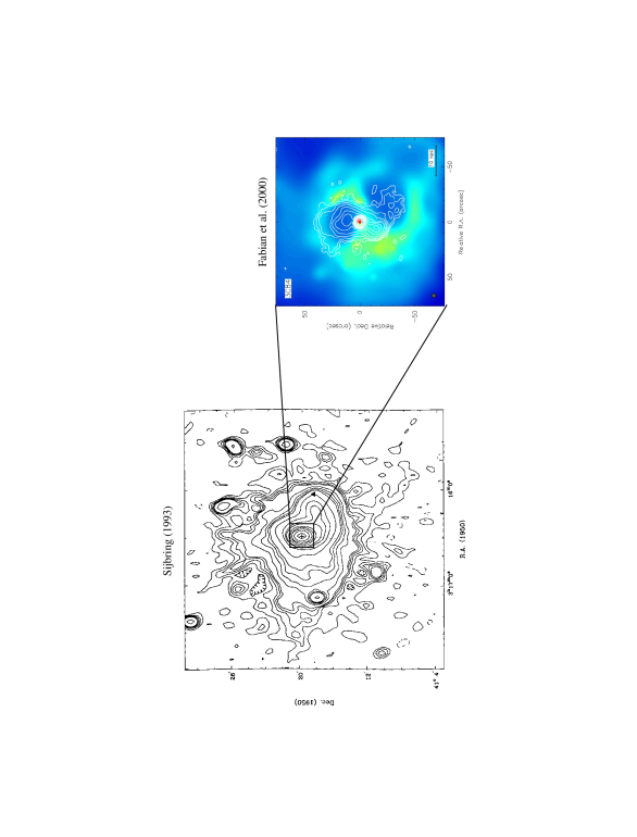
Figure 2: Left panel: 327 MHz map of the mini-halo in the Perseus cluster at a resolution of $51^{\prime\prime}\times 77^{\prime\prime}$ (Sijbring 1993). The cross indicates the position of the cD galaxy NGC 1275 and the dashed line represents the direction considered for the application of GBS’s model.  Right panel: X–ray (grey scale)/radio (contours) overlay for the central part of the Perseus cluster around NCG 1275 (Fabian et al. 2000); X–ray data are obtained with Chandra.

The most striking evidence in favour of our model is provided by the case of the Perseus cluster (A426, z=0.0183). The diffuse radio emission from the mini–halo (see left panel in Fig. 2) has a total extension of $\sim 15^{\prime}$ (at the redshift of the cluster $1^{\prime}$ corresponds to $\sim 30$ kpc) and its morphology is correlated with that of the cooling flow X-ray map (Sijbring 1993; Ettori, Fabian & White 1998).

On smaller scales ($\sim 1^{\prime}$), there is evidence of interaction between the radio lobes of the central radiogalaxy 3C84 and the X–ray emitting intra–cluster gas (e.g., Böhringer et al. 1993; Fabian et al. 2000; see Fig. 2, right panel). A recent interpretation is that the holes in the X–ray emission are due to buoyant radio lobes which are currently expanding subsonically (Churazov et al. 2000; Fabian et al. 2002). It is important to notice that the spectral index in these lobes ranges from $\sim 0.7$ in the center to $\sim 1.5$ in the outer regions (Pedlar et al. 1990), which is a value similar to the spectrum of the mini–halo extended over a scale $\sim 10$ times larger. Therefore, it is difficult to find a direct connection between the radio lobes and the large–scale mini–halo in terms of simple buoyancy or particle diffusion: the expansion and buoyancy of blobs would produce adiabatic losses and a decrease of the magnetic field causing a too strong steepening of the spectrum which would prevent the detection of large–scale radio emission. In addition, the diffusion time ($\propto R^{2}$, with $R=$ scale of interest; see also Sect. 3.2) is about 100 times longer than the radiative lifetime of the radio electrons.

Thus, if relativistic electrons are of primary origin, efficient re–acceleration mechanisms in the cooling flow region are necessary to explain the presence of the large–scale radio emission in Fig. 2; in particular, the detailed modelling of the radio properties of the mini–halo in Perseus (brightness profile, integrated spectrum and radial spectral steepening) resulted in good agreement with the data in case of isotropic compression of the magnetic field (GBS).

3 Abell 2626: a new mini–halo candidate?

Table 1: VLA Data Archive

Proj Code	Source	Observation	Frequency	Bandwidth	Array	TOS	RA (J2000)	Dec (J2000)
	Name	Date	(MHz)	(kHz)		(h)	(h m s)	(∘ ′ ′′)
AP001	3C464	Oct-22-1985	307.50/327.50	3.125	DnC	1.5	23 36 30	21 08 44
AR279	A2626	May-04-1993	327.50/333.00	3.125	B	0.3	23 36 30	21 08 44
AR279	A2626	Jul-15-1993	1464.900	5.000	C	0.5	23 36 30	21 08 44
ROLA	4C2057	Jul-20-1982	1464.900	5.000	B	0.7	23 36 30	21 08 06

The cluster A2626 hosts a relatively strong cooling flow (White, Jones & Forman 1997) and contains an amorphous radio source near to the center (Roland et al. 1985; Burns 1990) which is extended on a scale comparable to that of the cooling flow region with an elongation coincident with the X–ray distribution (Rizza et al. 2000).

X–ray image deprojection analysis of Einstein IPC derives a mass deposition rate $\dot{M}\sim 53\dot{\mbox{ M}}_{\odot}\mbox{ yr}^{-1}$, a cooling radius $r_{\rm c}\sim 114$ kpc and an average temperature $kT\sim 3.1$ keV (White, Jones & Forman 1997). From Soker & Sarazin (1990), one can estimate the proton number density at the cooling radius as:

$$n_{\rm c}\approx 2.18\times 10^{-3}\,\mbox{ cm}^{-3}\left(\frac{\dot{M}}{100\mbox{ M}_{\odot}\mbox{ yr}^{-1}}\right)\left(\frac{r_{\rm c}}{\mbox{100 kpc}}\right)^{-3}$$ (6)

so that $n_{\rm c}\sim 7.8\times 10^{-4}\mbox{ cm}^{-3}$ with the values of $\dot{M}$ and $r_{\rm c}$ for A2626.

3.1 VLA archive data analysis

In order to extend the application of GBS’s model to A2626, we have requested and analyzed some of the VLA archive data (Table LABEL:vladata.tab) of A2626 with the aim to derive the surface brightness map, the total spectral index and the spectral index distribution of the diffuse radio emission.

Figure 3: 1.5 GHz VLA map of A2626 at a resolution of $17^{\prime\prime}\times 17^{\prime\prime}$. The contour levels are $-0.06$ (dashed), 0.06, 0.12, 0.24, 0.48, 0.96, 1.92, 2.5, 4, 8, 10, 12 mJy/beam. The r.m.s. noise is 0.02 mJy/beam. The cross indicates the position of the cluster center.

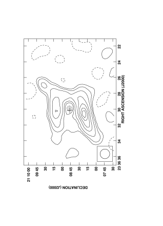
Figure 4: 330 MHz VLA map of A2626 at a resolution of $17^{\prime\prime}\times 17^{\prime\prime}$. The contour levels are $-8.5$ (dashed), 8.5, 17, 34, 68, 100, 135, 160 mJy/beam. The r.m.s. noise is 3.1 mJy/beam. The cross indicates the position of the cluster center and the dashed region defines the central brightness hole.

Standard data reduction was done using the National Radio Astronomy Observatory (NRAO) AIPS package. We used the 1.5 GHz C array data and the 330 MHz B+DnC array data to produce low resolution images with a circular restoring beam of 17 arcsec. The imaging procedure at each frequency was performed using data with matched uv coverage. These images (Fig. 3 and 4) allow to derive morphological and spectral information of the diffuse emission. The 1.5 GHz map (Fig. 3) shows an unresolved core and a diffuse boxy–shaped emission extended for $\sim 2^{\prime}$, corresponding to about 190 kpc. No significant polarized flux is detected, leading to a polarization upper limit of $<2$ %. An unrelated source is present to the west of the diffuse emission, with a total flux density of $\sim$3.9 mJy.

The diffuse structure at 330 MHz (Fig. 4) is smaller in extent, because of the lower sensitivity. It consists of two elongated almost parallel features located to the north and south of the core, respectively. No radio emission is detected at the location of the 1.5 GHz radio nucleus. Assuming for the 330 MHz core flux an upper limit of 3$\sigma$, we obtain that the radio core has an inverted spectrum (Table LABEL:risradio.tab). The total flux density of the diffuse emission is $S_{330}\sim 1$ Jy. The unrelated source, detected at 1.5 GHz to the west of the diffuse radio emission, is not detected at 330 MHz; this implies a spectrum with $\alpha^{1.5}_{0.3}$ $<$ $\sim$0.6.

In order to estimate the total integrated flux density of the diffuse radio emission at 1.5 GHz and derive the surface brightness map and spectral trend, it is necessary to subtract the emission from the central nuclear source. One way is to make a high–resolution image and then extract the clean components of the central source. By using the 1.5 GHz B array data we produced the high resolution image (Fig. 5) with a restoring beam of $4.5\times 3.9$ arcsec. The central component is found to consist of an unresolved core, plus a jet-like feature pointing to the south-western direction. The extended emission is resolved out and two elongated parallel features of similar brightness and extent are detected. The flux density of the central component, the short jet included, is $\simeq 13.5$ mJy, in agreement with Roland et al. (1985). The clean components of the central discrete source (jet included) were then restored with a circular beam of 17 arcsec and subtracted from the low–resolution map. This subtraction allows to derive a good estimate of the total flux density of the diffuse emission ($S_{1.5}\sim 29$ mJy).

As discussed in Sect. 3.2 and 3.3, we believe that the elongated structures visible in Fig. 5 are distinct (or that they may represent an earlier evolutionary stage) from the diffuse emission, and that the diffuse radio source may belong to the mini–halo class. The total flux density of these structures is $\sim 6.6$ mJy, thus contributing to only $\sim$ 20 % of the flux of the diffuse radio emission. Since we are interested in studying and modelling the diffuse radio emission, we produced a new low–resolution map at 1.5 GHz where these discrete radio features have been subtracted (Fig. 6). The subtraction procedure was similar to that used for the subtraction of the central discrete source. Of course the resulting map (Fig. 6) has a r.m.s. noise much higher than that of original map (Fig. 3). We notice that after the subtraction of the elongated features the morphology of the diffuse radio emission becomes roughly circular, thus warranting the application of a spherical model in Sect. 3.2. To be conservative, the region in which the surface brightness is affected by the central emission (within the dash–dotted circle in Fig. 6) has been excluded in modelling the diffuse radio emission (see Sect. 3.2).

Unfortunately, due to the lack of a high–resolution image, the two elongated features can not be subtracted at 330 MHz as well. Therefore, in deriving the spectral information of the diffuse emission we considered for consistency the low–resolution images in Fig. 3 and 4, which both include the contribution of the two features to the total flux.

The integrated spectral index of the diffuse emission between $\nu=330$ MHz and $\nu=1.5$ GHz is $\alpha\sim 2.4$. If the two features consist of relatively fresh injected plasma (as discussed in Sect. 3.3), their spectrum is expected to be relatively flat and thus the real spectrum of the diffuse emission would be slightly steeper ($\alpha\sim 2.5$ in the extreme case in which the two features do not contribute to the flux measured at 330 MHz).

In Fig. 7 we show a grey scale image of the spectral index map of the diffuse radio emission between $\nu=330$ MHz and $\nu=1.5$ GHz. The spectrum steepens from the central region towards the north and south direction, with the spectral index increasing from $\sim$1.2 to $\sim$3. The steepening in the northern region is slightly smoother than in the southern one.

Figure 5: 1.5 GHz VLA map of A2626 at a resolution of $4.5^{\prime\prime}\times 3.9^{\prime\prime}$. The contour levels are $-0.09$ (dashed), 0.09, 0.18, 0.36, 0.7, 1.4, 3, 5.5, 11, 20 mJy/beam. The r.m.s. noise is 0.03 mJy/beam

Figure 6: 1.5 GHz VLA map of A2626 at a resolution of $17^{\prime\prime}\times 17^{\prime\prime}$ after the subtraction of the two elongated features visible in Fig. 5. The cross indicates the position of the cluster center. The contour levels are $-0.18$ (dashed), 0.18, 0.36, 0.72, 1.2, 1.85, 2.3 mJy/beam. The r.m.s. noise is 0.08 mJy/beam. The dash–dotted circle defines the nuclear region excluded in modelling the diffuse radio emission, while the solid line represents the direction we have considered for the surface brightness profile (see Fig. 8).

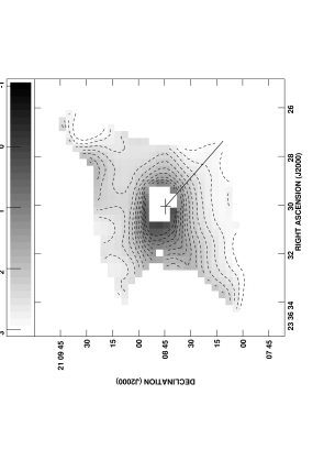
Figure 7: Spectral index distribution between $\nu=330$ MHz and $\nu=1.5$ GHz at a resolution of $17^{\prime\prime}\times 17^{\prime\prime}$. The contours are in steps of 0.2, where the lightest grey is in the range 2.8 to 3. The lighter the grey, the steeper the spectral index. We have excluded the region in which the error is $>0.2$. The cross indicates the position of the subtracted radio core and the solid line represents the direction we have considered for the spectral steepening profile (see Fig. 10).

Electrons emitting at frequencies $\sim$ 1 GHz in magnetic fields of the order of $\sim$ 1-3 $\mu$G (see Sect. 3.3) have a radiative lifetime (Eq. 1) $\sim 7\times 10^{7}$ yr.

The radio results are summarized in Table LABEL:risradio.tab.

Table 2: Radio results for A2626

Emission	$S_{330}$	$S_{1.5}$	Size	$\alpha$
	(mJy)	(mJy)	(arcsec2)	($S_{\nu}\propto\nu^{-\alpha}$)
Nuclear	$<$9.3	$13.5\pm 1.5$	-	$<$ $\sim$$-0.25$
Diffuse	$990\pm 50$	$29\pm 2$	$135\times 128$	$2.37\pm 0.05$

3.2 Model for A2626

As presented in Sect. 3.1, the extended radio source observed at the center of A2626 is characterized by amorphous morphology, lack of polarized flux and very steep spectrum which steepens with distance from the center. Finally, the morphology of the diffuse radio emission is similar to that of the cooling flow region (Rizza et al. 2000). These results indicate that the diffuse radio source may be classified as a mini–halo.

In addition, we notice that there are some concerns in interpreting this source without assuming the presence of particle re–acceleration. One possibility would be that the radio–emitting region is being supplied with fresh relativistic plasma that ultimately comes from the nucleus. Thus the observed diffuse radio emission would result from a bubble–like structures expanding into the surrounding cluster gas, as suggested for the large–scale radio structure of M87 presented by Owen, Eilek & Kassim (2000). Following the model adopted by these authors for M87, by assuming that the bubble pressure remains comparable to the external pressure (that is approximately constant in a cooling flow region, resulting $\sim 7.7\times 10^{-12}\mbox{ dyn cm}^{-2}$ at $r_{\rm c}$) we estimate that the age of the radio structure of A2626 at a radius $\sim$ 100 kpc would be $\sim 1.2\times 10^{9}\,P_{44}^{-1}$ yr (we adopted an internal adiabatic index of $\Gamma=4/3$ and the jet power $P$ in units of $10^{44}\mbox{ erg s}^{-1}$). We notice that, with a typical value $P_{44}\sim 1$, this age would be at least 10 times longer than the lifetime of the radio–emitting electrons, thus in situ acceleration would be necessary to energize the radio electrons. In addition we notice that this scenario is not able to explain the observed spectral steepening of the radio emission with distance. Another possibility, which instead may be able to explain a radial spectral steepening, would be particle diffusion out of the central region. The diffusion length is defined as $R_{\rm diff}\simeq\sqrt{6{\cal{K}}\tau_{\rm diff}}$ (e.g., Fujita & Sarazin 2001), where $\cal{K}$ is the spatial diffusion coefficient and $\tau_{\rm diff}$ the diffusion time. By assuming the commonly adopted Kolmogorov spectrum of the magnetic field it is possible to verify that for radio–emitting electrons (which typically have Lorentz factors $\gamma\sim 10^{4}$ and radiative lifetimes $\sim 10^{8}$yr) the diffusion length (by adopting the parallel diffusion coefficient, $\cal{K}_{\|}$) during their lifetime is $R_{\rm diff}$ $<$ $\sim$30 kpc (e.g., Brunetti 2003). This diffusion length is thus a factor 3 shorter than the scale of interest in the radio source of A2626 ($\sim 100$ kpc). As a consequence, diffusion may be an efficient process only for electrons with energy 10 times smaller than that of those responsible for the large–scale radio emission. Anomalous diffusion may considerably increase the propagation of electrons perpendicular to the magnetic field lines (e.g., Duffy et al. 1995). This kind of diffusion increases with increasing the turbulence energy density; however, the ratio between anomalous and parallel diffusion coefficients is (Giacalone & Jokipii 1999; Enßlin 2003) ${\cal{K}}_{\rm a}/{\cal{K}}_{\|}\sim 0.04(\delta B/B)^{4}$ and thus parallel diffusion still remains the most efficient way for particle diffusion also in the case of relatively powerful turbulence (i.e., $\delta B\sim B$). One possibility to enhance anomalous diffusion is to significantly increase the turbulence energy density and change, at the same time, the ratio between large–scale and small–scale turbulence. This possibility has been discussed in the literature to allow a more efficient escape of cosmic rays from the cocoon of radio sources (Enßlin 2003). However, given typical conditions in a cooling flow region, an unlikely high level of MHD turbulence should be injected (e.g., $\delta B/B\sim$ 15-20) in order to guarantee an electron diffusion length of $\sim 100$ kpc in $<10^{8}$ yr via enhanced anomalous diffusion, but this would also yield an extremely efficient particle acceleration via wave-particle scattering.

Given the above difficulties in explaining the amorphous radio structure observed in A2626, we apply GBS’s model. However, the application is not straightforward as in the case of Perseus because of the presence of the two structured radio features observed about $20^{\prime\prime}$ on either side of the nucleus in the high resolution image (Fig. 5), which may indicate that there is still some injection of relatively young ($\sim 10^{8}$ yr) relativistic plasma in the cooling flow region. This suggests that A2626 has physical properties in between those of the well known case of M87 (in which there is only marginal evidence for electron re–acceleration, e.g., Owen, Eilek & Kassim 2000) and of the prototype of mini–halo, in the Perseus cluster.

One important conclusion reached in the application of the GBS’s model to the Perseus cluster is that the results are compatible with the observations by assuming an isotropic compression of the magnetic field in the cooling flow region. This is consistent with the fact that the turbulent velocity results greater than the mean inflow velocity at the cooling radius, $v_{\rm F,c}\sim 21\left(\dot{M}/100\mbox{ M}_{\odot}\mbox{ yr}^{-1}\right)\left(r_{\rm c}/\mbox{100 kpc}\right)^{-2}\left(n_{\rm c}/10^{-3}\mbox{ cm}^{-3}\right)^{-1}\\ \mbox{km s}^{-1}$ (Soker & Sarazin 1990), and isotropic compression of the field is expected (Tribble 1993). By assuming a relatively powerful turbulence (i.e., $\delta B\sim B$), the turbulence energy density at the cooling radius is $\eta\,n_{\rm c}m_{\rm p}v_{\rm T,c}^{2}\sim B_{\rm c}^{2}/8\pi$ ($\eta<1$ is a fudge factor) and thus the velocity of the eddies of turbulence would be $v_{\rm T,c}\sim 90\,(B_{\rm c}/1.6\mu G)\,\eta^{-1/2}\,(n_{\rm c}/8\times 10^{-4}\mbox{cm}^{-3})^{-1/2}\mbox{ km s}^{-1}$. This value is greater than that of the mean inflow velocity of A2626 ($v_{\rm F,c}\sim 10\mbox{ km s}^{-1}$) and thus we considered only the case of an isotropic compression of the magnetic field.

Figure 8: Fit to the surface brightness profile (black circles) observed at 1.5 GHz along the radial direction indicated in Fig. 6. The dotted line defines the observed region of values of the brightness distribution at any radius, while the large dashed line represents the 2 r.m.s. noise level of the map subtracted from the elongated radio features (the errorbars are at 1$\sigma$). The fit is obtained with the following set of parameters: $B_{\rm c}=1.5\mu\mbox{G}$, $l_{\rm c}=175\mbox{ pc}$, $s=-0.5$. For comparison, we also report (with triangles) the brightness profile taken along the same radial direction from the 1.5 GHz map including the contribution of the elongated features (Fig. 3). The small dashed line represents the 2 r.m.s. noise level of the non–subtracted map.

We have already noticed that after the subtraction of the two elongated features, the morphology of the diffuse radio emission becomes roughly spherical (see Fig. 6), thus justifying the application to A2626 of GBS’s model, which indeed assumes spherical symmetry. In particular, in fitting the brightness profile we are authorized to choose a particular radial direction and give the deviations from the spherical symmetry in other directions with respect to the one considered.

In order to test the prediction of the model we have calculated the following expected observable properties:

total spectrum: the total synchrotron spectrum is obtained by integrating the synchrotron emissivity from an electron population with the energy distribution given by Eq. 5 over the cluster volume;

brightness profile: the surface brightness profile expected by the model is obtained by integrating the synchrotron emissivity at 1.5 GHz along the line of sight;

radial spectral steepening: at varying projected radius, we obtain the surface brightness at 330 MHz and 1.5 GHz, and compute the spectral index between these two frequencies.
The expected brightness profile and radial spectral steepening in the model are compared to the observed profiles along the radial direction indicated in Fig. 6 and 7. Since it is not possible to subtract the elongated features at 330 MHz (see Sect. 3.1), their contribution to the total spectrum is accounted for by the errorbars.

The values of the parameters required by the model to match the three observational constraints at the 90% confidence level are: $-1<s<0$, $B_{\rm c}\sim 1.2$ - $1.6\,\mu$G, $l_{\rm c}/(\delta B_{\rm c}/B_{\rm c})^{2}\sim 120$ - $180$ pc, where the lower $s$ corresponds to the lower $B_{\rm c}$ and $l_{\rm c}/(\delta B_{\rm c}/B_{\rm c})^{2}$. For these parameters, one obtains that the break energy at the cooling radius is $\gamma_{\rm b,c}\simeq 1100$. In Fig. 8, 9 and 10 we show the fits to the surface brightness profile, total spectrum and radial spectral steepening for one set of the parameters which best reproduces all the observational constraints.

Figure 9: Fit to the total spectrum of the synchrotron emission obtained with the same set of parameters of Fig. 8. The flux densities observed at 330 MHz and 1.5 GHz are taken from Table LABEL:risradio.tab, while the flux density at 609 MHz is obtained by subtracting the estimated core emission from the total flux given by Roland et al. (1985). The contribution of the elongated features to the flux of the diffuse emission (as estimated in Sect. 3.1) is included in the errorbars.

Figure 10: Fit to the radial spectral steepening between $\nu=330$ MHz and $\nu=1.5$ GHz obtained with the same set of parameters of Fig. 8. The data are taken from the spectral index distribution along the direction indicated in Fig. 7. The effect induced by the contribution of the elongated features to the flux of the diffuse emission (as estimated in Sect. 3.1) is included in the errorbars.

3.3 Discussion

The physical implications derived by applying GBS’s model to A2626 are discussed and compared with the results obtained for the Perseus cluster. For completeness the X–ray and radio data for these clusters are listed in Table LABEL:confr_dati.tab while the model results for both clusters are summarised in Table LABEL:confr_ris.tab.

It is worth pointing out that GBS’s model is able to reproduce all the observational constraints of A2626 for physically–meaningful values of the parameters (Table LABEL:confr_ris.tab). First of all we found that in the case of A2626 the range of values obtained for $B_{\rm c}$, although somewhat higher than that of Perseus, is in agreement with the measurements of magnetic field strengths in the ICM (Carilli & Taylor 2002 and references therein).

We also notice that the $l_{\rm c}/[\delta B_{\rm c}/B_{\rm c}]^{2}$ value required by the model for A2626 is higher than that found for Perseus (see column 3 of Table LABEL:confr_ris.tab). Even though we can not discriminate between the two contributions to this parameter, it is more likely that $[\delta B_{\rm c}/B_{\rm c}]^{2}$ in A2626 is smaller than in Perseus, as $l_{\rm c}$ depends on the micro–physics and is not expected to change considerably. In particular, in the general theory of turbulent plasma one can calculate the wavelength which carries most of the turbulent energy in a spectrum of Alfvén waves (e.g. Tsytovich 1972). When applied to the case of the ICM, with standard values of the physical parameters, it gives results of the order of tens to hundreds pc (GBS).

Table 3: Observational data for the cooling flow and mini–halo in Perseus and A2626

	X–RAY DATA					RADIO DATA
Cluster	$\dot{M}$	$r_{\rm c}$	$kT$	$n_{\rm c}$	$P_{\rm CF}$	$P_{1.5}$	$r_{\rm mh}$	$\alpha$
	($\mbox{M}_{\odot}\mbox{ yr}^{-1}$)	(kpc)	(keV)	($\mbox{cm}^{-3}$)	(erg s-1)	(W Hz-1)	(kpc)	($S_{\nu}\propto\nu^{-\alpha}$)
Perseus	$519^{+3}_{-17}$	$210^{+100}_{-20}$	$6.33^{+0.21}_{-0.18}$	$1.2\times 10^{-3}$	$2.6\times 10^{44}$	$4.4\times 10^{24}$	$\sim 300$	$\sim 1.2$
A2626	$53^{+36}_{-30}$	$114^{+50}_{-59}$	$3.1^{+0.5}_{-1}$	$7.8\times 10^{-4}$	$1.2\times 10^{43}$	$4.3\times 10^{23}$	$\sim 100$	$\sim 2.4$

Notes: Columns 2 and 3 list the cooling flow parameters, taken from Ettori, Fabian & White (1998) with ROSAT PSPC for Perseus and from White, Jones & Forman (1997) with Einstein IPC for A2626. Column 4 lists the average temperature of the ICM, taken from Allen et al. (1992) with Ginga for Perseus and from White, Jones & Forman (1997) with Einstein IPC for A2626. Column 5 lists the electron number density $n_{\rm c}$, estimated from Eq. 6. Column 6 lists the power supplied by the cooling flow as estimated from X–ray data by Eq. 3.3. Columns 7, 8 and 9 list the physical properties of the mini–halo: total power at 1.5 GHz, radius, and integrated spectral index between $\nu\sim 330$ MHz and $\nu\sim 1.5$ GHz. Radio data for Perseus are taken from Sijbring (1993).

Table 4: Model results for Perseus and A2626

	MODEL PARAMETERS			MODEL RESULTS
Cluster	$B_{\rm c}$	$l_{\rm c}/[\delta B_{\rm c}/B_{\rm c}]^{2}$	s	$\gamma_{\rm b,c}$	$N(\gamma_{\rm b})_{\rm c}\cdot\gamma_{\rm b,c}$	$E_{\rm e}$	$N_{\rm e}$	$P_{\rm e}$	$\epsilon$
	($\mu\mbox{G}$)	(pc)			($\mbox{cm}^{-3}$)	(erg)		(erg s-1)	(%)
Perseus	0.9 - 1.2	35 - 60	$\sim 2$	1600	$2.2\times 10^{-12}$	$1.6\times 10^{58}$	$1.6\times 10^{61}$	$8.9\times 10^{41}$	$0.34$
A2626	1.2 - 1.6	120 - 180	$\sim-0.5$	1100	$8.5\times 10^{-12}$	$2.2\times 10^{57}$	$3.2\times 10^{60}$	$8.3\times 10^{40}$	$0.69$

Notes: Columns 2, 3 and 4 list the parameters of the model derived by fitting all the observational constraints. Column 5, 6, 7, 8 and 9 list the physical properties derived by the model: respectively, the break energy of the electron spectrum at $r_{\rm c}$, the number density of electrons with energy $\gamma_{\rm b}m_{\rm e}c^{2}$ at $r_{\rm c}$, the energetics associated with the electrons re–accelerated in the cooling flow region (Eq. 7), their total number and the power necessary to re–accelerate them (Eq. 8). Column 10 lists the efficiency $\epsilon$ required by the cooling flow for re–accelerating the relativistic electrons, given in percentage of $P_{\rm CF}$ taken from column 6 of Table LABEL:confr_dati.tab. The results for Perseus are taken from GBS and modified according to Eq. 3 and 5. See text for details.

Concerning the energy density of the relativistic electrons, we find that it is approximately constant inside the cooling flow region ($s\sim 0$). Since $\gamma_{\rm b}$ depends very weakly on the radial distance, this means that the radial distribution of the number density of the electrons before the re–acceleration is nearly constant, producing a sort of “plateau” of relic electrons in the cooling flow region. On the other hand, in the case of Perseus, GBS found that the energy density of the relativistic electrons increases towards the center. A possible qualitative explanation of the “plateau” is that past radio activity may have released electrons in the cooling flow region. That this might be the case is suggested by the presence of the two extended features in Fig. 5 which, indeed, may be buoyant plumes recently ejected by the central source. As shown by several authors (e.g., Gull & Northover 1973; Churazov et al. 2000; Brüggen & Kaiser 2002), the outflow is accompanied by adiabatic expansion and further mixing of the energetic relativistic electrons with the ambient ICM; the time–scale of this process ($\sim 10^{7}$ - $10^{8}$ yr) is comparable to (or bigger than) the lifetime of the electrons producing synchrotron radiation. The disruption of the bubbles produced in past radio outbursts would then have left a population of relic relativistic electrons mixed with the thermal plasma in the cooling flow region. These relic electrons could diffuse in the thermal plasma up to $\sim 100$ kpc scale in a few Gyr (e.g., Brunetti 2003) filling the whole region inside the two elongated parallel features observed in Fig. 5, thus forming the “plateau” of relic electrons requested by our modelling.

Note that we found an electron distribution with $\gamma_{\rm b}\sim 10^{3}$. We stress that this is not inconsistent with the value $\gamma\sim 10^{4}$ adopted in the discussion of diffusion of radio–emitting electrons (Sect. 3.2), because a re–accelerated electron population with $\gamma_{\rm b}\sim 10^{3}$ is able to emit at GHz frequencies thanks to the shape of the re–accelerated spectrum which is peaked at $\sim\gamma_{b}$ (see Eq. 5), while the spectrum of non re–accelerated electrons (a power–law with a high energy cut–off at such a $\gamma_{\rm b}$) does not allow to emit efficiently in this band. As a consequence, without acceleration (i.e., simple diffusion model), electrons with $\gamma_{\rm b}\sim 10^{4}$ are necessary to account for the radio flux.

The energetics associated with the population of electrons re–accelerated in the cooling flow region can be estimated as:

$$E_{\rm e}\approx 23\frac{r_{\rm c}^{3}\,m_{\rm e}c^{2}N(\gamma_{\rm b})_{\rm c}\,\gamma_{\rm b,c}^{2}}{(3-s)}\;\;\;\mbox{erg}$$ (7)

where $N(\gamma_{\rm b})_{\rm c}$ is the number density (per $\gamma$ unit) of electrons with energy $\gamma_{\rm b}m_{\rm e}c^{2}$ at $r_{\rm c}$.

The total number of relativistic electrons can be estimated from the energetics as: $N_{\rm e}\sim 4E_{\rm e}/(3m_{\rm e}c^{2}\,\gamma_{\rm b,c})$.

With the model parameters found for A2626, one obtains $E_{\rm e}\sim 2.2\times 10^{57}$ erg and $N_{\rm e}\sim 3.2\times 10^{60}$. It is worth noticing that both the energetics and the number of electrons re–accelerated in the cooling flow region are about one order of magnitude smaller than those found in Perseus. This is consistent with the fact that the radio power of the mini–halo in A2626 is about one order of magnitude smaller than that in Perseus.

The power $P_{\rm e}$ necessary to re–accelerate the emitting electrons is given by the minimum energy one must supply to balance the radiative losses of these electrons: $P_{\rm e}\approx m_{\rm e}c^{2}\beta\,\gamma_{\rm b,c}^{2}\cdot N_{\rm e}$, where $\beta$ is the same as in Eq. 2. By assuming an average magnetic field in the cooling flow region of order $\sim 3\mu$G (this value is justified by considering the intensity $B_{\rm c}$ obtained in the model and the radial behaviour of field amplification expected in the case of isotropic compression), we obtain:

$$P_{\rm e}\approx 2\times 10^{-26}\,\gamma_{\rm b,c}^{2}\cdot N_{\rm e}\;\;\;\mbox{ erg s}^{-1}$$ (8)

which should be significantly smaller than the power supplied by the cooling flow. The maximum possible power $P_{\rm CF}$ which can be extracted from the cooling flow itself can be estimated assuming a standard cooling flow model and it corresponds to the $p\,dV/dt$ work done on the gas per unit time as it enters $r_{\rm c}$ : $P_{\rm CF}=p_{\rm c}\cdot 4\pi r_{\rm c}^{2}\cdot v_{\rm F,c}\sim 2/5L_{\rm cool}$ (e.g., Fabian 1994, $L_{\rm cool}$ being the luminosity associated with the cooling region). For typical values of the physical parameters in cooling flow clusters one has:

$$P_{\rm CF} \sim 2.3\times 10^{43}\left(\frac{n_{\rm c}}{10^{-3}\mbox{ cm}^{-3}}\right)\left(\frac{kT}{\mbox{6 keV}}\right)\left(\frac{r_{\rm c}}{\mbox{100 kpc}}\right)^{2}\cdot$$

$$\cdot \left(\frac{v_{\rm F,c}}{\mbox{10 km s}^{-1}}\right)\;\;\;\mbox{ erg s}^{-1}$$ (9)

In the case of A2626, one obtains that the power necessary to re–accelerate the relic electrons is $P_{\rm e}\sim 8.3\times 10^{40}$ erg s^-1, while the power supplied by the cooling flow is $P_{\rm CF}\sim 1.2\times 10^{43}$ erg s^-1. Therefore, only a small fraction ($\sim 0.7$ %) of $P_{\rm CF}$ should be converted into electron re–acceleration, and thus we conclude that processes powered by the cooling flow itself are able to provide sufficient energy to power the radio mini–halo in A2626. A similar result is found for Perseus (see column 10 of Table LABEL:confr_ris.tab).

4 Observational properties of mini–halos

With the aim to explore the properties of mini–halos we selected a small sample of candidates among known diffuse radio sources in the literature. The clusters in the sample were selected based on the presence of both a cooling flow and a diffuse radio emission with no direct association with the central radio source. In particular, since GBS’s model assumes a connection between the origin of the synchrotron emission and the cooling flow, to be conservative we selected those clusters where the size of the diffuse radio emission is comparable to the cooling radius. For this reason we excluded Abell 2052, the Virgo cluster and 2A 0335+096, which host amorphous radio sources with a size considerably smaller than the cooling flow region. Relevant X–ray and radio data are reported in Tab. LABEL:minialoni.tab, along with references, while in Fig. 11 we report the radio power at 1.4 GHz of the mini–halos (in terms of integrated radio luminosity $\nu P_{\nu}$) versus the maximum power of the cooling flows $P_{\rm CF}=\dot{M}kT/\mu m_{\rm p}$. A general trend is found, with the strongest radio mini—halos associated with the most powerful cooling flows.

Table 5: Observational data for mini–halos

Cluster	$z$	$\dot{M}$	$kT$	$P_{1.4}$
		($\mbox{M}_{\odot}\mbox{ yr}^{-1}$)	(keV)	(W Hz-1)
PKS 0745-191	0.1028	$579^{+399}_{-215}$	$8.3^{+0.5}_{-5.8}$	$2.7\times 10^{25}$
Abell 2390	0.2320	$625^{+75}_{-75}$	$9.5^{+1.3}_{-3.4}$	$1.5\times 10^{25}$
Perseus	0.0183	$283^{+14}_{-12}$	$6.3^{+1.5}_{-2.3}$	$4.4\times 10^{24}$
Abell 2142	0.0890	$106^{+248}_{-106}$	$11.4^{+0.8}_{-3.2}$	$6.6\times 10^{23}$
Abell 2626	0.0604	$53^{+36}_{-30}$	$3.1^{+0.5}_{-1.0}$	$4.3\times 10^{23}$

References: X–ray data: Perseus, A2142, A2626: White, Jones & Forman (1997) with Einstein IPC; PKS 0745-191: White, Jones & Forman (1997) with Einstein HRI; A2390: $\dot{M}$ from Böhringer et al. (1998) with ROSAT PSPC, $kT$ from White, Jones & Forman (1997) with Einstein IPC. Radio data: PKS 0745-191: Baum & O’Dea (1991); A2390: Bacchi et al. (2003); Perseus: Sijbring (1993); A2142: Giovannini & Feretti (2000); A2626: this work.

Figure 11: Integrated radio power at 1.4 GHz, $\left[\nu P_{\nu}\right]_{\rm 1.4GHz}$, vs. cooling flow power, $P_{\rm CF}=\dot{M}kT/\mu m_{\rm p}$, for the mini–halo clusters in Tab. LABEL:minialoni.tab.

Since for A2626 the only available X-ray observation is from Einstein IPC, for consistency the X–ray data were taken, when possible, from the compilation of White, Jones & Forman (1997) with Einstein Observatory. For A2390, not detected as a cooling flow cluster by Einstein IPC, the value of $\dot{M}$ is taken from more recent observations with ROSAT PSPC, which have shown the presence of a cooling flow in this cluster (Böhringer et al. 1998). Note that when both measurements from Einstein and ROSAT are available (e.g., Perseus, A2142, PKS 0745 -191), the Einstein–based $\dot{M}$ is a factor $\sim$ 2 below the ROSAT–based value.

We notice that the maximum powers which can be extracted from cooling flows are orders of magnitude larger than the integrated radio powers (see Fig. 11), in qualitative agreement with the very low efficiencies calculated in the model (see column 10 of Table LABEL:confr_ris.tab).

As already discussed in Sect. 2, it is worth noticing that new Chandra and XMM–Newton results obtained for a limited number of objects hint to an overestimate of $\dot{M}$ derived by earlier observations: in particular, the consensus reached in these studies (e.g., McNamara et al. 2000; Peterson et al. 2001; David et al. 2001; Tamura et al. 2001; Molendi & Pizzolato 2001; Böhringer et al. 2001; Peterson et al. 2003) is that the spectroscopically–derived cooling rates are a factor $\sim$ 5-10 less than earlier ROSAT and Einstein values (e.g., Fabian & Allen 2003). This factor seems to be similar for all clusters in a large range of $\dot{M}$, giving a systematic effect that will not spoil the correlation reported in Fig. 11.

In addition, we stress that the trend seen in Fig. 11 is expected in the framework of GBS’s model. Qualitatively, $P_{\rm radio}\propto\langle\gamma_{\rm b}\rangle^{2}\,{\mathcal{N}}_{\gamma_{\rm b}}\,\langle B\rangle^{2}\,r_{\rm c}^{3}$, where $\langle\gamma_{\rm b}\rangle$ and $\langle B\rangle$ are the average values of gamma break and magnetic field in the cooling flow region, while $\mathcal{N}_{\gamma_{\rm b}}$ is the number density of relativistic electrons with Lorentz factor $\gamma=\gamma_{\rm b}$. We remind that the bulk of the observed radio emission is indeed produced by the electrons with Lorentz factor $\gamma\sim\gamma_{\rm b}$. On the other hand, the maximum power which can be extracted from a cooling flow estimated on the basis of a standard cooling flow model is $P_{\rm CF}=p_{\rm c}\cdot 4\pi r_{\rm c}^{2}\cdot v_{\rm F,c}$ (see Sect. 3.3), where $v_{\rm F,c}\propto\dot{M}\,r_{\rm c}^{-2}\,n_{\rm c}^{-1}$ (Fabian, Nulsen & Canizares 1984). Thus from Eq. 6 one has: $P_{\rm CF}\propto p_{\rm c}\,r_{\rm c}^{3}$ and, since cooling flows are pressure–constant processes, it results: $P_{\rm CF}\propto r_{\rm c}^{3}$, i.e. $P_{\rm radio}$ is expected to increase with $P_{\rm CF}$, with an efficiency $\epsilon$ which depends on details (related to the micro–physics of the complicated parameterization of $P_{\rm radio}$) not considered in the model.

The trend presented in Fig. 11 is based on few objects with still relatively large errors on the parameters. If true, this trend would clearly indicate a connection between the thermal ICM and the relativistic electrons in cooling cores in qualitative agreement with our theoretical expectations. It should be stressed that we may have introduced a bias in our sample since, in order to deal with objects belonging to the radio mini–halo class, we have selected only those objects with an extension similar to that of the cooling flow region. These are well developed radio mini–halos which would have a relatively high efficiency in the particle acceleration process. The trend between radio and cooling flow powers in Fig. 11 may thus result from the fact that the efficiency of the particle acceleration is similar in the selected clusters.

In general, the efficiency in converting the cooling flow power into particle acceleration depends on relatively unknown quantities : the energy transport from large–scale turbulence towards the smaller scales, and the details of the coupling between the turbulence at small scales and the relativistic electrons. All these quantities depend on microphysics and it may likely be that this would lead to a situation of broad ranges of efficiencies.

If low efficiency radio mini–halos exist, they will fill the bottom–right corner of Fig. 11. These objects may be less extended and fainter than typical mini–halos. In addition, it may likely be that the electrons in these objects are not re–accelerated to the energies necessary to produce $\sim$ GHz synchrotron emission, and thus that they would emit only at much lower frequencies. It is evident that future surveys of radio mini–halos in cooling flow clusters combined with X–ray studies of the ICM would shed new light on the link between thermal and relativistic plasma in clusters and on the physics of turbulence and particle acceleration in these regions.

5 Conclusions

We have reported a detailed study of the radio properties of a new mini–halo candidate in A2626. We have shown that a particle re–acceleration model (GBS’s model) with a set of physically–meaningful values of the parameters is able to account for the observed brightness profile, the integrated synchrotron spectrum and the radial spectral steepening. We conclude that A2626 has physical properties in between the case of M87, for which there is only marginal evidence for electron re–acceleration, and the prototype of mini–halos in the Perseus cluster. Moreover, we obtain that the maximum power of the cooling flow is more than 2 orders of magnitude larger than the emitted radio power, thus indicating that the cooling flow power (even if considerably reduced by the recent observational claims) may play a leading role in powering the radio mini–halo.

We have selected a small sample of well developed radio mini–halos and shown that the radio power of these objects correlates to the cooling flow power. GBS’s model for particle re–acceleration in cooling flow is consistent with the observed trend. If confirmed, in the re–acceleration scenario this trend would indicate that the conversion of the cooling flow power into magneto–plasma turbulence and particle acceleration is similar in well developed radio mini–halos.

- (1) Allen, S. W., Fabian, A. C., Johnstone, R. M., Nulsen, P. E. J., & Edge, A. C. 1992, MNRAS, 254, 51
- (2) Bacchi, M., Feretti, L., Giovannini, G., & Govoni, F. 2003, A&A, 400, 465
- (3) Baum, S. A., & O’Dea, C. P. 1991, MNRAS, 250, 737
- (4) Böhringer H., Voges W., Fabian A. C., Edge A. C., & Neumann D. N. 1993, MNRAS, 264, L25
- (5) Böhringer H., Tanaka, Y., Mushotzky, R. F., Ikebe, Y., & Hattori, M. 1998, A&A, 334, 789
- (6) Böhringer, H., Belsole, E., Kennea, J., Matsushita, K., Molendi, S., et al. 2001, A&A, 365, 181
- (7) Brüggen, M., & Kaiser, C., 2002, Nature, 418, 301
- (8) Brunetti, G., Setti, G., Feretti, L., & Giovannini, G. 2001, MNRAS, 320, 365
- (9) Brunetti, G. 2003, Proceedings of the Conference on Matter and Energy in Clusters of Galaxies held on April 23–27 2002 in Chung-Li, Taiwan; ASP Conf. Series, 301, 349, eds. S. Bowyer & C.-Y. Hwang
- (10) Burns J. O. 1990, AJ 99, 14
- (11) Burns J. O., Sulkanen M. E., Gisler G. R., Perley R. A. 1992, Ap.J.Lett., 388, L49
- (12) Carilli, C. L., & Taylor, G. B. 2002, ARA&A, 40, 319
- (13) Churazov, E., Forman, W., Jones, C., & Böhringer, H. 2000, A&A, 356, 788
- (14) David, L. P., Nulsen, P. E. J., McNamara, B. R., Forman, W., Jones, C., et al. 2001, ApJ, 557, 546
- (15) Duffy, P., Kirk, J.G., Gallant, Y.A., & Dendy, R.O., 1995, A&A, 302, L21
- (16) Edge A.C., 2001, MNRAS, 328, 762
- (17) Edge A.C., Stewart G.C., & Fabian A.C. 1992, MNRAS, 258, 177
- (18) Enßlin, T., 2003, A&A, 399, 409
- (19) Ettori S., Fabian A. C., & White D. A. 1998, MNRAS, 300, 837
- (20) Fabian, A. C. 1994, ARA&A, 32, 277
- (21) Fabian, A. C., Nulsen, P. E. J., & Canizares, C. R. 1984, Nature, 310, 733
- (22) Fabian, A. C., Sanders, J. S., Ettori, S., Taylor, G. B., Allen, S. W., et al. 2000, MNRAS, 318, 65
- (23) Fabian, A. C., Celotti A., Blundell K. M., Kassim N. E., & Perley R. A. 2002, MNRAS, 331, 369
- (24) Fabian, A. C., & Allen, S. W. 2003, to appear in the Proceedings of the XXI Texas Symposium on Relativistic Astrophysics held on December 9–13 2002, in Florence, Italy [astro–ph/0304020]
- (25) Feretti, L., & Giovannini, G. 1996, IAUS, 175, 333
- (26) Fujita, Y., & Sarazin, C. L., 2001, ApJ, 563, 660
- (27) Ge, J.P., & Owen, F.N. 1993, AJ, 105, 3
- (28) Giacalone, J., & Jokipii, J. R., 1999, ApJ, 520, 204
- (29) Giovannini, G. & Feretti, L. 2000, NewA 5, 335
- (30) Giovannini, G. & Feretti, L. 2002, in Merging Processes in Clusters of Galaxies, ed. L. Feretti, I. M. Gioia, G. Giovannini (Dordrecht: Kluwer)
- (31) Gitti, M., Brunetti, G., & Setti, G. 2002, A&A, 386, 456 (GBS)
- (32) Gull, S. F., & Northover, K. J. E. 1973, Nature, 244, 80
- (33) McNamara, B. R., Wise, M., Nulsen, P. E. J., David, L. P., Sarazin, C. L, et al. 2000, ApJ, 534, L135
- (34) Melrose D. B. 1980, Plasma Astrophysics: Nonthermal Processes in Diffuse Magnetized Plasmas, Gordon and Breach
- (35) Molendi, S., & Pizzolato, F. 2001, ApJ, 560, 194
- (36) Owen, F. N., Eilek, J. A., & Kassim, N. E. 2000, ApJ, 543, 611
- (37) Pedlar, A., Ghataure, H. S., Davies, R. D., et al. 1990, MNRAS, 246, 477
- (38) Peterson, J. R., Paerels, F. B. S., Kaastra, J. S., Arnaud, M., Reiprich, T. H., et al. 2001, A&A, 365, 104
- (39) Peterson, J. R., Kahn, S. M., Paerels, F. B. S., Kaastra, J. S., Tamura, T., et al. 2003, ApJ, 590, 207
- (40) Pfrommer, C, & Enßlin, T. 2003, A&A in press [astro-ph/0306257]
- (41) Rizza E., Loken C., Bliton M., Roettiger K., & Burns J.O. 2000, AJ, 119, 21
- (42) Roland, J., Hanish, R. J., Véron P., & Fomalont, E. 1985, A&A, 148, 323
- (43) Salomé, P., & Combes, F., 2003, astro-ph/0309304
- (44) Sarazin C.L. 2002, in Merging Processes in Clusters of Galaxies, eds. L. Feretti, I. M. Gioia, G. Giovannini (Dordrecht: Kluwer)
- (45) Schlickeiser, R., Sievers, A., & Thiemann, H., 1987, A&A, 182, 21
- (46) Sijbring, D. 1993, Ph.D. Thesis, Groningen
- (47) Soker, N., & Sarazin C.L. 1990, ApJ, 348, 73
- (48) Tamura, T., Kaastra, J. S., Peterson, J. R., Paerels, F. B. S., Mittaz, J. P. D., et al. 2001, A&A, 365, L87
- (49) Tribble, P.C. 1993, MNRAS, 263, 31
- (50) White, D. A., Jones, C., & Forman, W. 1997, MNRAS, 292, 419