Combined Long and Short Timescale X-ray Variability of NGC 4051 with RXTE and XMM-Newton

Abstract

We present a comprehensive examination of the X-ray variability of the narrow line Seyfert 1 (NLS1) galaxy NGC 4051, one of the most variable AGN in the sky. We combine over 6.5 years of frequent monitoring observations by RXTE with a $>100$ ks continuous observation by XMM-Newton and so present an overall 2-10 keV powerspectral density (PSD) covering an unprecedent frequency range of over 6.5 decades from $<10^{-8}$ to $>10^{-2}$ Hz. The combined RXTE and XMM-Newton PSD is a very good match to the PSD of the galactic black hole binary system (GBH) Cyg X-1 when in a ‘high’, rather than ‘low’, state providing the first definite confirmation of an AGN in a ‘high’ state. We also find that a bending powerlaw, rather than a sharply broken powerlaw, besides being more physical, is a much better description of the high state PSD of Cyg X-1 and is also a better description of the PSD of NGC 4051.

At low frequencies the PSD of NGC 4051 has a slope of -1.1 bending, at a frequency $\nu_{B}=8^{+4}_{-3}\times 10^{-4}$Hz, to a slope of $\alpha_{H}\sim-2$. Although $\nu_{B}$ does not depend on photon energy, $\alpha_{H}$ is steeper at lower energies. If $\nu_{B}$ scales with mass, we imply a black hole mass of $3^{+2}_{-1}\times 10^{5}M_{\odot}$ in NGC 4051, which is consistent with the recently reported reverberation value of $5^{+6}_{-3}\times 10^{5}M_{\odot}$. Hence NGC 4051 is emitting at $\sim 30\%\rm~{}L_{Edd}$.

NGC 4051 follows the same rms-flux relationship as GBHs, consistent with higher Fourier frequencies being associated with smaller radii.

From the cross-powerspectra and cross-correlation functions between XMM-Newton lightcurves in different energy bands, we note that the higher energy photons lag the lower energy ones. We also note that the lag is greater for variations of longer Fourier period and increases with the energy separation of the bands. Variations in different wavebands are very coherent at long Fourier periods but the coherence decreases at shorter periods and as the energy separation between bands increases. This behaviour is again similar to that of GBHs, and of MCG-6-30-15, and suggests a radial distribution of frequencies and photon energies with higher energies and higher frequencies being associated with smaller radii.

Combining our observations with observations from the literature we find it is not possible to fit all AGN to the same linear scaling of break timescale with black hole mass. However broad line AGN are consistent with a linear scaling of break timescale with mass from Cyg X-1 in its low state and NLS1 galaxies scale better with Cyg X-1 in its high state. We suggest that the relationship between black hole mass and break timescale is a function of at least one other underlying parameter which may be accretion rate or black hole spin or both.

1 INTRODUCTION

Early observations with EXOSAT showed that, on short timescales (day to minutes) AGN X-ray variability was quasi-scale invariant, with power spectral densities (PSDs) being reasonably described by simple powerlaws or perhaps slightly curving functions (Lawrence et al. 1987; M^cHardy and Czerny 1987). However examination of archival data (M^cHardy 1988) showed that, on longer timescales ($\mathrel{\hbox{\hbox to0.0pt{\hbox{\lower 4.0pt\hbox{$\sim$}}\hss}\hbox{$>$}}}$weeks) the scale invariance of at least one AGN, NGC 5506, broke down and its PSD flattened below a bend, or ‘knee’ frequency of $\sim 10^{-6}$Hz. The combined long and short timescale PSD of NGC 5506 resembled that of galactic black hole X-ray binary systems (GBHs) such as Cyg X-1 (eg Nowak et al. 1999) which, when in a ‘low’ state, has a ‘knee’ frequency of $\sim 0.2$Hz, below which the PSD flattens to a slope of zero. If the knee frequencies scale with mass, then a reasonable black hole mass in NGC 5506 of $\sim$few $\times 10^{6}M_{\circ}$ was implied. Thus the possibility arose of determining AGN black hole masses from observations of long timescale X-ray variability.

Again using a variety of archival data, Papadakis and M^cHardy (1995) demonstrated that the PSD of the brighter AGN, NGC 4151, also flattened at low frequencies ($<10^{-7}$Hz) but long term X-ray lightcurves remained of poor quality until the launch of the Rossi X-ray Timing Explorer (RXTE; Swank 1998) in December 1995. RXTE can sample on sub-daily timescales and so, since shortly after launch we, and other groups, have been monitoring a small sample of AGN in order to produce high quality long timescale PSDs. One of our main targets is NGC 4051 and results from the first 1.5 years of observation (M^cHardy et al. 1998) indicated that the slope at low frequencies was probably flatter than that at high frequencies but neither the break frequency, or the slopes, were particularly well defined. Edelson and Nandra (1999), Pounds et al. (2001) and Markowitz et al. (2003) have all now demonstrated PSD flattening in other AGN at low frequencies, using RXTE data.

Although RXTE provides much better long term X-ray lightcurves than any previous observatory, the lightcurves are still not continously sampled, or even completely uniformly sampled. Thus the ‘raw’ or ‘dirty’ PSDs will be contaminated by artefacts which depend on the window sampling pattern. In order to overcome such problems we have developed a simulation-based modelling process (Uttley, M^cHardy and Papadakis 2002) which can determine not only the value of any break frequencies, or PSD slopes, but can also derive errors for these parameters, and also quantify the goodness of fit of any model. Uttley et al. (2002) applied this method to the first 3 years of observations of four AGN. They found evidence for bends, or breaks, in the PSDs in three AGN, NGC 5506, NGC 3516 and MCG-6-30-15, although not in NGC 5548.

GBHs are found in a variety of ‘states’ (eg McClintock and Remillard 2003; Cui et al. 1997a), the most common of which are the so called low flux, hard spectrum (or ‘low’) state, and the high flux, soft spectrum (or ‘high’) state. In the standard Comptonisation models for the production of X-ray emission, different physical regimes apply to low and high states, with a higher seed photon flux in the high state, leading to a cooler Comptonising corona (eg Zdziarski et al. 2002). If we are to attempt physical modelling of AGN we therefore need to know which state they are in. For GBHs, the PSDs of the high (eg Cui et al. 1997b, Churazov et al. 2001) and low (eg Nowak et al. 1999; Revnivtsev, Gilfanov and Churazov 2000) states are different, thereby providing us with a means of discrimination.

In Cyg X-1 in the low state, the PSD slope above the ‘knee’ (refered to above, at $\sim 0.2$Hz) is $\sim-1$. However at $\sim 3$Hz there is a second, higher frequency, break above which the PSD slope is $\sim-2$. In the high state only one break has been detected so far in the PSD of Cyg X-1. The break frequency is $\sim 10-20$Hz and, above the break, the PSD slope is steeper than -2. Below the break the PSD has a slope of -1 for at least 4 decades of frequency (Reig et al. 2002).

For AGN, there are two cases (Akn 564, Papadakis et al. 2002 and NGC 3783, Markowitz et al. 2003) where two breaks have been found, indicating a possible similarity to low state systems. However in most other AGN only one break has been found and, although the slopes below the break are not that well defined (eg Uttley et al. 2002; Markowitz et al. 2003), in general they are closer to -1 than to zero. However it is not clear whether these breaks correspond to the high frequency break in low state systems or the single break in high state systems.

If we assume that timescales scale approximately with mass, then to properly compare AGN with GBHs we require AGN PSDs which cover timescales from $\sim$few years to tens of seconds. RXTE monitoring observations principally sample timescales from $\sim$few years to $\sim$day but XMM-Newton can provide continous observations of up to almost 2 days with sampling on $\sim$second, or shorter, timescales. NGC 4051 is the AGN which is best observed on long timescales by RXTE and is also one of the best observed on short timescale with XMM-Newton. Here we present a combined PSD analysis of these two datasets.

In Section 2 we describe the observations and the data analysis procedures. In Section 3 we discuss the combined RXTE and XMM-Newton PSD, covering more than 6 decades in frequency, and compare it to that of GBHs, particularly Cyg X-1, in different states. As further diagnostics of the Comptonisation process we discuss the high frequency XMM-Newton data in more detail, and note that a similar analysis of a long XMM-Newton observation of MCG-6-30-15 has been carried out by Vaughan, Fabian and Nandra (2003), producing broadly similar results. In Section 3 we note a variation of PSD slope with photon energy at high frequencies. In Section 6 we determine the rms-flux relation (Uttley and M^cHardy 2001) from the XMM-Newton data. We discuss the relationship between variations in different wavebands both in terms of the cross-correlation function (Section 7) and using cross-spectrum phase spectrum analysis (Section 8). In Section 9 we discuss the coherence of the variations between different wavebands, ie whether the same variations occur in all bands or whether there are independent contributions in different wavebands. In Section 10 we summarise the main observational results from this paper. Finally, in Section 11, we compare NGC 4051 with high and low state GBHs and discuss possible physical models for the X-ray emission region. We also examine the relationship between PSD break timescale and black hole mass in AGN, noting that the relationship is probably different for broad and narrow line Seyfert 1 galaxies, perhaps because of a difference in mass accretion rate or spin.

2 OBSERVATIONS AND DATA REDUCTION

2.1 RXTE

Here we present (Fig. 1) all of the short ($\sim$1 ks duration) monitoring observations of NGC 4051 which have been carried out with the proportional counter array (PCA, Zhang et al. 1993) on RXTE from 1996 until 2002 inclusive. As the gain of the PCA, and the number of PCUs, has varied throughout the lifetime of the instrument, we derive here a lightcurve in flux units rather than in counts so that all observations may be used together. This ‘flux’ lightcurve is used in all subsequent analysis.

During periods when the gain, and number of PCUs did not change, the flux and count rate lightcurves are identical, indicating no significant contribution from variable absorption to the variability above 2 keV which is seen by RXTE. (We also note that, in their detailed study of the X-ray spectral variability of NGC 4051 with RXTE, Lamer et al. (2003a) find no evidence that the time averaged spectral variations are caused by variable absorption. Also from RXTE observations Taylor et al. (2003) find that the X-ray spectral variability of NGC 4051 is well explained by pivoting of the X-ray spectrum about a high energy ($\sim 100$ keV) and do not require any variations of absorbing column.)

Changes in luminosity can alter the ionisation state of warm gas in the line of sight to AGN such as NGC4051 (eg M^cHardy et al. 1995) and so can affect the transparency of the gas. Such changes do not affect significantly the spectrum above 2 keV and are mainly restricted to lines from carbon, oxygen, nitrogen and neon below 2 keV. However, as we see from the XMM-Newton reflection grating spectrum (Ogle et al. 2003) which was taken at the same time as the XMM-Newton imaging observations described below, the total absorption below 2 keV in those lines in NGC4051 is only a few percent of the total continuum flux. Therefore variations in that few percent would be small and could not account for the large flux variations seen in Fig. 2. Thus the flux variations described in this paper represent variations in the continuum source and not in any absorbing gas.

The PCA consists of 5 Xenon-filled proportional counter units (PCUs) sensitive to X-rays with energies between 2 and 60 keV. The maximum effective area of the PCA is 6500 cm². For each observation we extracted the Xenon 1 (top) layer data from all PCUs that were switched on during the observation as layer 1 provides the highest S/N for photons in the energy range 2-20 keV where the flux from AGN is strongest. We used FTOOLS v4.2 for the reduction of the PCA data and extracted source spectra according to the standard method outlined in Lamer et al. (2003b). We used standard ‘good time’ data selection criteria, i.e. target elevation $>10^{\circ}$, pointing offset $<0.01^{\circ}$, time since SAA passage $>30$min and standard threshold for electron contamination. We calculated the model background in the PCA with the tool PCABACKEST v2.1 using the L7 model for faint sources. PCA response matrices were calculated individually for each observation using PCARSP V2.37, taking into account temporal variations of the detector gain and the changing number of detectors used. Fluxes in the 2-10 keV band were then determined using XSPEC, fitting a simple powerlaw with variable slope but with absorption fixed at the Galactic level of $1.3\times 10^{20}$ cm^-2 (Elvis, Lockman and Wilkes 1988; Stark et al. 1992; M^cHardy et al. 1995). The errors in the flux are scaled directly from the observed errors in the measured count rate.

As can be seen from Fig. 1, a variety of sampling patterns were undertaken. In the first four AOs, prior to 2000, we used a quasi-logarithmic sampling pattern, covering all timescales, but rather economically. In order to improve the S/N on our resulting PSDs, and to improve our understanding of other phenomena such as ‘low’ states (eg Guainazzi et al. 1998; Uttley et al. 1999), and of the relationship between the X-ray and optical flux variations (Peterson et al. 2000; Shemmer et al. 2003), we then increased our coverage. From 2000 onwards, our minimum observation frequency has been once every two days. In addition, to sample properly the higher frequencies, we observed every 6 hours for 2 months in 2000.

Figure 1: RXTE Long Term 2-10 keV lightcurve of NGC 4051. Each data point represents an observation of $\sim 1$ ks.

2.2 XMM-Newton

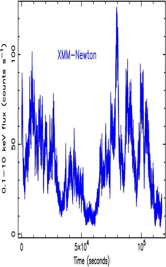
Figure 2: XMM-Newton background-subtracted lightcurve of NGC 4051 in the 0.1-10 keV energy band, with 5s time bins, combining data from both PN and MOS CCDs.

NGC 4051 was observed for a complete XMM-Newton orbit over the 16th and 17th May 2001. The EPIC PN and MOS2 cameras were operated in small window modes with medium filters, while MOS1 was in timing mode with the thin filter. The PN and MOS cameras took data continuously for 117 ks and 107 ks respectively. Background levels were low in all 3 detectors for the first 103 ks, after which the background began to flare due to increased levels of soft protons, affecting the lightcurves significantly at high energies ($>$5 keV).

The data were processed and lightcurves were produced using the XMM-Newton Standard Analysis System (SAS) version 5.2. The PN source+background lightcurve was obtained from a 42 arcsecond radius circle centred on the source, and the background lightcurve was taken from two similar sized source-free regions on the same chip. The MOS2 source+background lightcurve was taken from a 45 arcsecond circle centred on the NGC 4051 and the background lightcurve was obtained from source-free regions of the inner parts of the outer chips. The MOS1 source+background lightcurve was obtained from a 52-pixel wide region of the timing window centred on the source and the background lightcurve was taken from a 26-pixel wide strip at the edge of the timing window.

The PN detector in small window mode, and MOS1 in timing mode, have negligible pileup at the typical flux of NGC 4051 and, apart from a difference in S/N, the lightcurves are the same within the errors. However MOS2, in small window mode, is slightly affected by pileup. An empirical correction for pileup, of up to 10% at the highest countrates, in the MOS2 lightcurve was therefore obtained by comparison with the MOS 1 and PN lightcurves. After applying this time-averaged correction, the MOS2 and PN lightcurves are the same within the errors. The background subtracted and (for MOS2) pileup corrected lightcurves were then summed to produce combined lightcurves of the highest possible S/N. The resulting full band (0.1-10 keV) lightcurve is shown in Fig. 2. As the full 0.1-10 keV lightcurve is dominated by photons of low energy, whose background level is not greatly affected by the proton flare referred to above, we show the full 117 ks of the observation in Fig. 2. However, for consistency, we restrict analysis, in all bands, to the first 102.5 ks of the observation, when the hard bands are not affected by increased background.

The XMM-Newton lightcurves, which we binned at 5s resolution, contain a small number ($\sim 14$) of short gaps. With the exception of one gap of 105s and another of 200s, all gaps have durations $\leq 35$s with most being $\leq 20$s. If left in, as zero counts, these gaps introduce a very small amount of spurious high frequency power into the PSDs and very slightly flatten it at frequencies $<10^{-2}$Hz. We have therefore filled these gaps by linear interpolation and the addition of noise characteristic of the surrounding datapoints. As the gaps are so small, and have such a small effect on the PSD (as one can see by inserting similar gaps elsewhere into the XMM-Newton lightcurves), the difference between linear interpolation and any other reasonable interpolation is undetectable. We therefore work in the rest of this paper with these lightcurves, whose units are ‘counts s^-1’, as their continuous nature simplifies some of the later analysis.

3 Powerspectral Analysis

3.1 Analysis Method

In order to model reliably the PSD of our data, taking into account the distorting effects of gaps in the observed RXTE light curves, together with red-noise leak effects, we use the Monte Carlo simulation based psresp method of Uttley et al. (2002). psresp is based on the earlier ‘response method’ of Done et al. (1992), which simulates red-noise lightcurves assuming a given PSD model and the observed sampling pattern, and compares the resulting model PSD with the observed PSD. psresp additionally allows PSDs measured from a number of lightcurves covering a range of time-scales to be combined, as is required here. Furthermore, the psresp method uses the distribution of best fitting $\chi^{2}$ of the simulated PSDs to estimate reliably the confidence for the null hypothesis that the assumed PSD model is correct. We refer the reader to Section 4 of Uttley et al. (2002) for a full discussion of the psresp method. In the context of that discussion, we note the following features of our psresp analysis of the XMM-Newton and RXTE PSDs:

1. For ease of computation we made two RXTE lightcurves, to cover long (years - month) and medium (month - day) timescales. The long timescale lightcurve is made from the entire RXTE monitoring lightcurve, binned up to 2-week resolution. The medium timescale lightcurve is made from only the two-month-long section of 6 hourly sampling and is binned to exactly 6 hour resolution. The binned lightcurves are very complete. Apart from a 200 day period at the end of 1999/beginning of 2000 where there are 9 observations instead of 14, there are no gaps. During the 64 day period of the 6 hourly sampling there are 247, rather than 256, observations. However during periods when there were 3 rather than 4 observations per day, the 3 observations were fairly evenly spaced. In both cases the few empty bins are filled by linear interpolation from adjacent bins. From the XMM-Newton data we made a lightcurve binned to 500 s resolution to make a high-frequency PSD, which is also included in the simulations. Since it is computationally prohibitive to simulate lightcurves at the full 5 s resolution of our XMM-Newton lightcurves, we insert directly into psresp the very high frequency (VHF: $10^{-3}$–$2\times 10^{-2}$ Hz) part of the PSD which is made from the full resolution lightcurve. This PSD is binned logarithmically into bins of frequency width $1.5\nu$, with errors determined in the conventional way, using the method of Papadakis & Lawrence (1993). The errors are well-determined due to the many cycles sampled at each frequency. As the observations are continuously sampled to frequencies above those included in the VHF PSD, where Poisson noise is dominant, aliasing is not a problem. Similarly, as the lightcurve samples frequencies well below those included red noise leak is not a problem.

2. For a given PSD model we simulated evenly sampled lightcurves, using the method of Timmer and Konig (1995), with time resolutions of 6 hours, 36 minutes and 500 s for the long and medium timescale RXTE lightcurves and the XMM-Newton lightcurve respectively. These lightcurves were then resampled to match the observed sampling pattern. The simulated RXTE lightcurves were then rebinned to the same resolution (2 weeks and 6 hours) as the observed lightcurves.

3. Both simulated and observed PSDs are binned up in logarithmically spaced frequency intervals of width $\nu\rightarrow 1.5\nu$. Poisson noise levels are added to the simulated PSDs together with the ‘aliased’ contribution expected due to variations shorter than the time resolution of the simulated light curves (see Uttley et al. 2002 for details).

4. For each set of PSD model parameters tested we simulate $N=300$ realisations for each of the three lightcurves included in the fit. For each of these three lightcurves we actually simulate one long lightcurve of length $300$ times the length of the observed lightcurve, and then split it into sections, thereby reducing red noise leakage problems. We therefore assume no power on timescales longer than $300\times$ the length of each of the contributing lightcurves, ie about 2000 years for the longest lightcurve. We use $M=3000$ random combinations of the simulated PSDs (plus realisations of the VHF PSD) to compare with the model average PSDs, in order to determine the distribution of $\chi^{2}$ expected for the given model (see Uttley et al. 2002, Section 4.2). Comparison with the observed $\chi^{2}$ yields a probability $P$ that the model is acceptable. Following the practice of Uttley et al. 2002, we define ‘absolute’ 90% errors on all model parameters, based on the parameter values which bracket the region of the parameter grid which is acceptable at $P>0.1$.

3.2 PSD of the NGC 4051 RXTE Data

As the long timescale PSD covers a large frequency range, it provides a first indication of whether NGC 4051 might be more like a low or high state system. We therefore modelled the RXTE data on its own, treating it as two separate lightcurves of 6 hour and 2 week resolution, as described above.

We first fitted the simplest model, ie a single unbroken powerlaw. That model turned out to be an excellent fit to the RXTE data (Fig. 3). The powerlaw slope, over the frequency range $7\times 10^{-9}$ to $2\times 10^{-5}$Hz was $-1.05^{+0.15}_{-0.20}$ and the fit probability was 0.93. (Throughout this paper we quote 90% confidence errors unless stated otherwise.) There was therefore no justification for fitting more complex models to that frequency range.

The large frequency range, fitted by a slope of -1.05, indicates that NGC 4051 may very well be a high state system. Therefore before making more complex fits, including the XMM-Newton data, we re-examine high state observations of Cyg X-1 in order to obtain a good PSD template with which we may compare the PSD of NGC 4051.

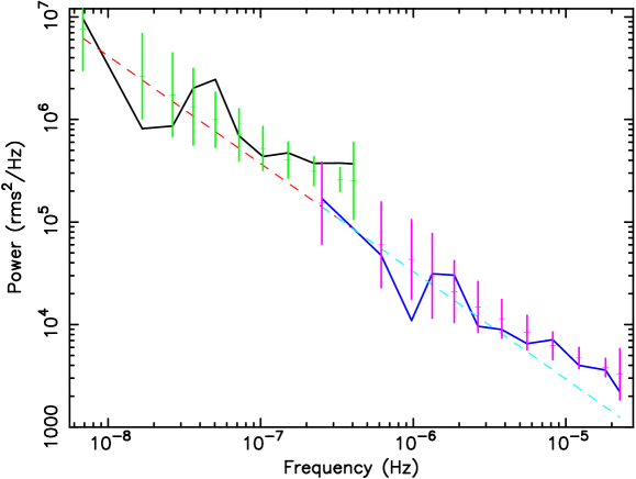
Figure 3: PSD of NGC 4051 using RXTE data only. The underlying single powerlaw model is the straight dashed line. The distorted model is given by the points with errorbars and the observed data is given by the two continuous solid lines. The best-fit powerlaw slope is $-1.05^{+0.15}_{-0.20}$ and the fit probability is 93%

4 The High State PSD of Cygnus X-1

4.1 Calculation of the Cyg X-1 High State PSD

Figure 4: PSD of Cyg X-1 in the high state in the 2-13 keV range. The dashed line is a powerlaw with an exponential cut-off and the solid line is a bending powerlaw, as described in the text. The upper frequency of the fits was 80Hz, but the fits have been extrapolated to higher frequencies. Although the bending powerlaw is a marginally better fit, both models are formally good fits.

Figure 5: $\delta\chi^{2}$ residuals for the best fitting sharply broken powerlaw (see text for parameters) to the PSD of Cyg X-1 shown in Fig. 4, fitting over the same frequency range. Note the large systematic deviations near the break frequency (13.9 Hz).

Cyg X-1 is the archetypal GBH against whose PSD the PSDs of AGN are usually compared. We should therefore determine first which model best describes the high state PSD of Cyg X-1 and then test that model against our observations of NGC 4051. A high state PSD of Cyg X-1 has been published by Revnivtsev et al. (2000) from RXTE proposal P10512 (see also Cui et al. 1997b). Revnivtsev et al. find that, below 15-20 Hz, the PSD has a slope of -1 and at higher frequencies the slope steepens to $\sim-2$. However they do not attempt to fit a single continuous model to the whole frequency range ($\sim 10^{-3}$ to $\sim$ few$\times 10^{2}$Hz) covered by the RXTE observations. We have therefore recalculated the high state PSD. We used PCA standard binned mode data from a single-orbit RXTE observation of Cyg X-1 in the high state (Observation ID 10512-01-09-01, observed 1996 June 18) and produced lightcurves in the 2-5 keV, 5-8 keV, 8-13 and 2-13 keV bands. (Note, sensitivity is low below 2.5 keV). The lightcurves are continuous and the resultant PSDs are not distorted noticeably by the window function and so can be considered to be a good representation of the true underlying PSDs. The final PSDs were obtained by averaging the PSDs measured from 128 s segments of the lightcurve and, when there is more than one frequency in a bin, binning in logarithmic frequency intervals $\nu\rightarrow 1.05\nu$. We estimated standard errors in each frequency bin using the spread in individual powers about the mean, and applied the deadtime correction formula of Sunyaev & Revnivtsev (2000) to the Poisson noise level to obtain Poisson-noise-subtracted PSDs. The PSDs from this observation are fairly typical of those obtained in the high state in this source (Cui et al. 1997b). The PSDs in various bands look rather similar and so we show, in Fig. 4, just the broad band 2-13 keV PSD.

4.2 Modelling of the Cyg X-1 High State PSD

Discontinuous broken powerlaws of the form

$$P(\nu)\propto\nu^{\alpha_{L}}\mbox{ for $\nu<\nu_{B}$ and}$$

$$P(\nu)\propto\nu^{\alpha_{H}}\mbox{ for $\nu>\nu_{B}$}$$

are often used to describe PSDs. In the present case, such a fit to the full 2-13 keV PSD gives $\alpha_{L}=-1.025\pm 0.013$, $\nu_{b}=13.9\pm 0.8$ and $\alpha_{H}=-2.13\pm 0.06$. These values are very similar to those derived by Revnivtsev et al. ( $\alpha_{low}\sim-1$, $\alpha_{high}\sim-2.1$, $\nu_{b}\sim 10-20$). However the fit is poor, particularly around the break frequency ($\chi^{2}=242/134\,dof$, ie P $<0.1\%$, see Fig. 5). It is clear that a smooth curve rather than a sharp break describes Fig. 4 better. We have therefore fitted two smoothly curving functions to the PSD. The dashed line in Fig. 4 is the best fit of a powerlaw with an exponential cut-off. The solid line is the best fit of a function which smoothly changes from one powerlaw to another. Below we give the form of that function which can accomodate any number of joined powerlaws where the powerlaw at low frequencies bends smoothly to become a steeper powerlaw at higher frequencies.

$$P(\nu)=A\nu^{-\alpha_{1}}\,\Pi_{i=1}^{N}\,\left(1+\left(\frac{\nu}{\nu_{b_{i}}}\right)^{(\alpha_{i+1}-\alpha_{i})}\right)^{-1}\,$$

Table 1: BENDING POWERLAW FITS TO CYG X-1

Energy Band	Normalisation (A)	$\alpha_{L}$	$\alpha_{H}$	$\nu_{B}$	$\chi^{2}/dof$
(KeV)				(Hz)
2-5	$5.44\times 10^{-3}$	$-0.939\pm 0.026$	$-2.72\pm 0.20$	$20.1\pm 2.2$	124/134
5-8	$1.00\times 10^{-2}$	$-0.945\pm 0.026$	$-2.87\pm 0.26$	$21.9\pm 2.3$	135/134
8-13	$1.19\times 10^{-3}$	$-0.943\pm 0.024$	$-3.18\pm 0.35$	$23.7\pm 2.2$	136/134

Table 2: BENDING POWERLAW FITS TO CYG X-1 WITH FIXED $\alpha_{L}=-0.94$

Energy Band	Normalisation (A)	$\alpha_{H}$	$\nu_{B}$	$\chi^{2}/dof$
(KeV)			(Hz)
2-5	$5.44\times 10^{-3}$	$-2.72\pm 0.14$	$20.2\pm 1.1$	124/135
5-8	$1.00\times 10^{-2}$	$-2.84\pm 0.19$	$21.5\pm 1.2$	135/135
8-13	$1.19\times 10^{-3}$	$-3.16\pm 0.28$	$23.5\pm 1.4$	136/135

In the present case we use it to describe just one break in the PSD ($N=$ number of breaks), and we refer to it as a bending powerlaw fit. The parameter, $A$, is the power at 1 Hz, assuming $\nu_{B}>>1$Hz, or the power extrapolated from the lowest frequency powerlaw if there is a break below, or near to, 1 Hz. $A$ is refered to in a number of following Tables as the normalisation. We have not used quite as much data as Revnivtsev et al. and have not attempted, as they did, to improve on the deadtime correction of Sunyaev & Revnivtsev. We therefore only fit models to the PSD up to 80Hz. However we plot extrapolations of the fits to higher frequencies. Although the bending powerlaw is a slightly better fit to the data ($\chi^{2}$=129/134 dof, P=61%), the bending powerlaw and exponential cut-off ($\chi^{2}$=140/135 dof, P=35%) are both formally good descriptions of the data, from $<10^{-2}$Hz to 80Hz. For the bending powerlaw fit, the low frequency slope $\alpha_{low},=-0.96\pm 0.02$, the break frequency $\nu_{b},=22.9\pm 1.5$Hz and the high frequency slope, $\alpha_{high},=-2.99\pm 0.14$. For the exponential cut-off fit the low frequency slope $\alpha_{low},=-0.89\pm 0.02$ and the break frequency $\nu_{b},=23.7\pm 1.1$Hz. We note that although the details of the fits vary, both the exponential and bending powerlaw fits agree on the value of $\nu_{b}$.

Revnivtsev et al. who calculate the high state PSD of Cyg X-1 up to $>$200 Hz, favour a powerlaw description of the highest frequency part of the PSD above the break. As a bending powerlaw is also the best fit to the PSDs which we have calculated, we therefore chose that model as our standard parameterisation of the high state PSD of Cyg X-1.

4.3 Variation of Cyg X-1 High State PSD shape with energy

The parameters of the fits of the bending powerlaw to the three energy bands in Cyg X-1 are given in Table 1. It can be seen that $\alpha_{low}$ is the same in all fits to within the errors. In order to reduce the errors on the other parameters, further fits have therefore been made with $\alpha_{low}$ fixed (at -0.94). The results of these fits are given in Table 2. From that table we can see that the high frequency slope, $\alpha_{H}$, becomes slightly steeper and $\nu_{B}$ increases slightly at higher energies although we caution that $\nu_{B}$ is towards the upper edge of the measurable frequency range and so $\alpha_{H}$ is not well constrained.

As $\alpha_{H}$ and $\nu_{B}$ are correlated in any fitting process, we have performed separate fits, additionally fixing either $\alpha_{H}$ (Table 3) or $\nu_{B}$ (Table 4). In the first case we still note a slight increase of $\nu_{B}$ with increasing energy and in the second case we note a very slight steepening of $\alpha_{H}$ with increasing energy. The changes between bands are small. For example in Table 4 we see that the range of $\alpha_{H}$ is only 0.2, which is about the same as the 90% confidence error on each measurement. More detailed observations are therefore needed to clarify whether these changes are real. If they are real then we note that they are in the opposite sense to that found for GBHs in the low state (eg Cyg X-1, Nowak et al. 1999) where the PSD at high frequencies (2-90 Hz, ie above the high frequency break) becomes less steep with increasing photon energy.

5 Combined RXTE and XMM-Newton Powerspectrum of NGC 4051

5.1 PSD in 2-10 keV Band

Figure 6: Combined RXTE and XMM-Newton (4-10 keV) PSD covering 6.5 decades of frequency. The underlying model is the thin dashed line. The distorted model is given by the points with errorbars and the observed data is given by the four continuous solid lines. The two lower frequency datasets ($7\times 10^{-9}$ to $2\times 10^{-5}$Hz) are from RXTE and the two higher frequency datasets ($\sim 10^{-5}$ to $\sim 10^{-3}$Hz and $\sim 10^{-3}$ to $\sim 10^{-2}$Hz) are from XMM-Newton. See the text for a more detailed description. Note that the Poisson noise has not been subtracted from the distorted model or the observed data as the noise level is included as part of the fitting process. Thus the PSD flattens at the highest frequencies.

In this section we calculate the combined long and short timescale PSD of NGC 4051 by combining long timescale data from RXTE and short timescale data from XMM-Newton. As stated earlier (Section 2) the gain of the RXTE PCA detectors, and the number of PCUs is not constant. We therefore cannot make useful continuous lightcurves in units of counts s^-1 and so make lightcurves in flux units, in the 2-10 keV band. The median photon energy of that band is 5.1 keV. As the PSD shape may be a function of photon energy (eg Nowak et al. 1999) we ensure that the median photon energy of the XMM-Newton lightcurve which we combine with the RXTE lightcurve is approximately the same. As XMM-Newton has a much softer response than RXTE, the closest approximation to the RXTE 2-10 keV band is the XMM-Newton 4-10 keV band, which has a median energy of 4.9 keV.

The RXTE lightcurves are simulated in the same way as is described in Sections 3.1 and  3.2, and the XMM-Newton lightcurves are treated as is described in Section 3.1. Overall we arrange the binning of the various lightcurves to ensure that there is almost no overlap of the resultant parts of the final PSD, which is shown in Fig. 6. This PSD is the best PSD yet obtained for any AGN and is visually quite similar to the high state PSD of Cyg X-1 which is shown in Fig. 4. A quantitative comparison of these PSDs is discussed below in Section 5.2.

Table 3: BENDING POWERLAW FITS TO CYG X-1 WITH FIXED $\alpha_{L}=-0.94$, $\alpha_{H}=-3.0$

Energy Band	Normalisation (A)	$\nu_{B}$	$\chi^{2}/dof$
(KeV)		(Hz)
2-5	$5.27\times 10^{-3}$	$21.3\pm 0.9$	134/136
5-8	$0.99\times 10^{-2}$	$22.0\pm 1.1$	137/136
8-13	$1.20\times 10^{-3}$	$23.3\pm 1.4$	137/136

Table 4: BENDING POWERLAW FITS TO CYG X-1 WITH FIXED $\alpha_{L}=-0.94$, $\nu_{B}=22.0$Hz

Energy Band	Normalisation (A)	$\alpha_{H}$	$\chi^{2}/dof$
(KeV)		(Hz)
2-5	$5.27\times 10^{-3}$	$-2.84\pm 0.13$	132/136
5-8	$0.99\times 10^{-2}$	$-2.88\pm 0.17$	135/136
8-13	$1.20\times 10^{-3}$	$-3.05\pm 0.25$	139/136

As a test of whether there is any significant problem with red noise leakage in the XMM-Newton VHF PSD, we have compared the results of including the XMM-Newton data in two separate ways. Firstly we treat the XMM-Newton data as a combination of a 500s binned lightcurve and a VHF PSD, as described in Section 3.1. Secondly we include the XMM-Newton data simply as a PSD of the full 5s binned XMM-Newton lightcurve, covering $\sim 10^{-5}$ to $\sim 2\times 10^{-2}$Hz, without any simulation of a 500s binned lightcurve. The combined RXTE and XMM-Newton model fits are the same in both cases to within the errors indicating that even without simulating the longer timescales present in the XMM-Newton data, the raw XMM-Newton PSD is untroubled by red noise leakage. Thus the VHF PSD is completely free of such problems. Below we discuss only the results obtained by including, with the RXTE data, the XMM-Newton data as a combination of a 500s binned lightcurve and a VHF PSD.

5.2 Model Fitting

We first fitted a simple powerlaw to the PSD. The PSD slope is -1.25 but the fit is poor (P=2.7%).

We therefore next tried the bending powerlaw model which best fits the Cyg X-1 high state. This model is a very good fit (best fit probability = 76%). The best fitting low frequency slope, $\alpha_{L}=-1.1$, the break frequency, $\nu_{B}=5\times 10^{-4}$Hz and the high frequency slope, $\alpha_{H}=-1.9$. The data are quite consistent with the values of $\alpha_{L}=-1$ and $\alpha_{H}=-2$ which Revnivtsev et al. (2000) use to describe the high state of Cyg X-1. The best model fit and confidence contours for combinations of these three parameters are given in figures 6, 7, 8 and 9.

We note that, although a very good fit is obtained with the above parameters, it is not the only reasonable fit. A possible fit is obtained with a much lower break frequency. However with a very low break frequency (ie $\sim 10^{-6}$Hz) we also require a high frequency slope which is close to the best fitting low frequency slope given above, and little difference between $\alpha_{L}$ and $\alpha_{H}$. This possible fit is another indication that most of the frequency range of the combined RXTE and XMM-Newton PSD is explained by a slope not far different from $\sim-1.1$, although there may be some slight curvature at the lowest observable frequencies.

Although a bending powerlaw is a much better fit to the Cyg X-1 data, for comparison we have fitted the previously commonly used sharply breaking powerlaw to the combined XMM-Newton and RXTE data. A good fit is obtained (P=82%) with $\nu_{B}=2.4\times 10^{-4}$Hz ($90\%$ confidence limits of $2.4\times 10^{-6}$ to $1.5\times 10^{-3}$Hz), $\alpha_{L}=-1.1^{+0.4}_{-0.1}$ and $\alpha_{H}=-1.8^{+0.4}_{-0.8}$. The high and low frequency slopes are very similar to those found using the bending powerlaw model but $\nu_{B}$ is lower and is not particularly tightly constrained.

The overall conclusion is that a single powerlaw is not a good fit, and two powerlaws are required, but the parameters of any bending or breaking powerlaw are not well defined.

Figure 7: 68%, 90% and 99% confidence contours for low frequency slope, $\alpha_{L}$, and break frequency, $\nu_{B}$, for bending powerlaw fit to the combined RXTE and XMM-Newton 4-10 keV PSD. Note here we plot $-\alpha_{L}$ to simplify the labels.

Figure 8: 68%, 90% and 99% confidence contours for high frequency slope, $\alpha_{H}$, and break frequency, $\nu_{B}$, for bending powerlaw fit to the combined RXTE and XMM-Newton 4-10 keV PSD. Following Fig. 7 we plot $-\alpha_{H}$.

Figure 9: 68%, 90% and 99% confidence contours for low and high frequency slopes, $\alpha_{L}$ and $\alpha_{H}$ respectively for bending powerlaw fit to the combined RXTE and XMM-Newton 4-10 keV PSD. Again we plot $-\alpha_{L}$ and $-\alpha_{H}$.

5.3 Variation of $Fvar$ with Energy for NGC 4051

In Table 5 we summarise the variability detectable in the various XMM-Newton bands. In column 2 we give the average counts/sec (‘Ave’), and in column 3 we give what is known as $Fvar$, ie the square root of the noise-subtracted variance, divided by the average count rate. These values of $Fvar$ have been calculated from lightcurves which were binned up to 100s in order to cut down the possibility of spurious contributions to the noise (which must be subtracted from the variance) from frequencies at which the PSD is completely dominated by Poisson noise. We see that $Fvar$ decreases with photon energy, above 2 keV. A similar decrease of variability with increasing photon energy in AGN has been reported in the past by Green, M^cHardy and Lehto (1993), Nandra et al. 1997, Turner, George and Nandra (1998) and Markowitz and Edelson (2001).

The interpretation of this result is not unique. One possibility, suggested by Green et al. , is that there is a relatively constant component of hard spectrum. That spectrum would not greatly affect the softer bands but would dilute the variability in the harder bands. That interpretation is consistent with the extremely hard component seen in a very low flux state (Guainazzi et al. 1998; Uttley et al. 1999). However Markowitz and Edelson (2001) claim, in their sample of AGN, that the decrease in variability with increasing energy is too strong to be explained only by the presence of a constant hard component. Alternatively, if in a Comptonisation scenario the bulk of the variability were provided by the seed photons, the greater number of scatterings required to raise photons to higher energies should wash out high frequency variability, but is contrary to the observations shown below (Section 5.4). However Taylor et al. (2003) show that the X-ray spectral variability of NGC 4051 is best described by pivoting of the X-ray spectrum about a high energy ($\sim 100$ keV), which automatically leads to a reduction in $Fvar$ with increasing energy (at least below the pivot energy). In the Comptonising models of Zdziarski et al. (2002) spectral pivoting is explained if the corona is responsible for dissipation of most of the accretion energy and its luminosity remains constant whilst the seed photon luminosity varies.

We note that $Fvar$ continues to rise down to energies below 1 keV. We also note that the 2-10 keV flux measured by RXTE varies in almost exactly the same way as the 0.1 keV flux seen by EUVE (Uttley et al. 2000), except that the amplitude of variability of the EUVE flux was slightly greater than that of the RXTE flux, consistent with spectral pivoting extending to quite low energies, and with the rise in $Fvar$ to low energies. Thus although the shape of the spectrum below 2 keV in NGC 4051 is more complex than a simple powerlaw (Salvi 2003 and Salvi et al. 2003; Uttley et al. 2003) the large majority of the low energy flux appears to vary, which is different from Cyg X-1 in the high state where there is a strong soft component which does not vary greatly.

However in the very lowest energy bin (0.1-0.5 keV) $Fvar$ actually decreases very slightly. Uttley et al. (2003) show that there is a relatively constant component in NGC 4051 at low as well as high (Taylor et al. 2003) energies and this component, although small, may account for the slight decrease in $Fvar$.

Table 5: Variation of $Fvar$ with Energy for NGC 4051

Energy Band	Ave	$Fvar$
keV	c s-1
0.1-0.5	17.8	0.51
0.5-1	11.7	0.54
1-2	7.6	0.52
2-5	3.3	0.40
5-10	0.8	0.27

5.4 Variation of High Frequency PSD Shape of NGC 4051 with Energy

We have produced PSDs, using just the XMM-Newton data, in a variety of spectral bands in order to investigate the spectral dependence of the PSD shape. We have already shown that the observed XMM-Newton PSDs derived here represent very closely the true PSDs. We can then remove the Poisson noise analytically and fit the bending powerlaw model to the noise-subtracted PSDs. The fits, allowing all parameters to be free, are given in Table 6. The fitting was carried out within the plotting package, QDP. We note that although the fits to the various XMM-Newton PSDs look quite good visually (eg Figs. 10 and 11), the formal fits are not particularly good for the lower energy bands where the errors on the PSD datapoints are smaller. In those bands the main contribution to the reduced $\chi^{2}$s comes from 2 or 3 datapoints with very small errors. For any sort of smooth continuous function without sharp breaks, or additional components such as QPOs, these data points prevent us from obtaining a better fit to the 0.1-2 keV PSD with any other model. Further observations would clarify the reality of the deviations from a smooth function but for the moment we can only assume that the deviations are a statistical fluctuation.

The errors on the parameters, allowing all to be free, are quite large and so we next fix $\alpha_{L}$ at -1.1, the best fit value from the joint RXTE and XMM-Newton fit. The resultant fits are given in Table 7. From that Table we can see that $\nu_{B}$ does not change with energy, to within the errors, but the high frequency slope steadily flattens as we move to higher energies. (The exception is the 5.0-10.0 keV band, but there are few photons in that band and the errors on all parameters are very large.)

In addition to the five relatively narrow spectral bands listed at the top of Tables 6 and 7, we calculate the PSD in two broader bands, 0.1-2.0 and 2.0-10.0 keV, in order to improve the statistical significance of the fits, which are given at the bottom of Tables 6 and 7. The noise-subtracted PSDs themselves are shown in Figs. 10 and 11. We can see immediately that the two PSDs are similar below $\sim 10^{-3}$Hz but, at higher frequencies, the 0.1-2 keV PSD is much steeper. However both PSDs have approximately the same value of $\nu_{B}\sim 8\times 10^{-4}$Hz.

We can see, from Figs 10 and 11 and Table 7, that although the high frequency PSD slope is steeper in the lower energy band, the normalisation of the PSD is larger. If the normalisations and break frequencies were the same, the steepening of the PSD would give rise to a lower value of $Fvar$ at lower energies. We therefore note that it is the higher normalisation of the PSD at lower energies which accounts for the higher value of $Fvar$.

Table 6: BENDING POWERLAW FITS TO XMM-Newton PSD OF NGC 4051

Energy Band	Normalisation (A)	$\alpha_{L}$	$\alpha_{H}$	$\nu_{B}$	$\chi^{2}/dof$
(KeV)				(Hz)
0.1-0.5	$2.90\times 10^{-2}$	$-1.04^{+0.6}_{-0.5}$	$-2.75^{+0.2}_{-0.4}$	$5.5^{+8}_{-3}\times 10^{-4}$	18.4/8
0.5-1.0	$3.54\times 10^{-3}$	$-1.27^{+0.5}_{-0.4}$	$-2.80^{+0.4}_{-0.7}$	$12^{+24}_{-8}\times 10^{-4}$	11.1/8
1.0-2.0	$9.14\times 10^{-2}$	$-0.94^{+0.9}_{-*}$	$-2.15^{+0.2}_{-0.5}$	$3.2^{+23}_{-2}\times 10^{-4}$	14.6/8
2.0-5.0	$4.10\times 10^{-4}$	$-1.45^{+0.4}_{-*}$	$-3.28^{+2.2}_{-3.5}$	$64^{+89}_{-61}\times 10^{-4}$	6.5/8
5.0-10.0	$4.40\times 10^{-3}$	$-1.13^{+0.5}_{-*}$	$-3.11^{+1.1}_{-1.7}$	$16^{+22}_{-13}\times 10^{-4}$	11.9/8
0.1-2.0	$8.80\times 10^{-3}$	$-1.16^{+0.5}_{-0.4}$	$-2.86^{+0.3}_{-0.4}$	$8.8^{+11}_{-4}\times 10^{-4}$	19.4/8
2.0-10.0	$3.21\times 10^{-4}$	$-1.47^{+0.3}_{-*}$	$-4.09^{+*}_{-*}$	$71^{+47}_{-53}\times 10^{-4}$	6.9/8

^∗ The error is large and no reliable value could be determined.

Table 7: BENDING POWERLAW FITS TO XMM-Newton PSD OF NGC 4051 WTIH FIXED $\alpha_{L}=-1.1$

Energy Band	Normalisation (A)	$\alpha_{H}$	$\nu_{B}$	$\chi^{2}/dof$
(KeV)			(Hz)
0.1-0.5	$1.76\times 10^{-2}$	$-2.77^{+0.2}_{-0.2}$	$5.9^{+3}_{-2}\times 10^{-4}$	18.4/9
0.5-1.0	$1.48\times 10^{-2}$	$-2.69^{+0.2}_{-0.3}$	$8.6^{+4}_{-4}\times 10^{-4}$	11.5/9
1.0-2.0	$2.08\times 10^{-2}$	$-2.21^{+0.2}_{-0.3}$	$4.5^{+5}_{-3}\times 10^{-4}$	14.8/9
2.0-5.0	$1.08\times 10^{-2}$	$-2.04^{+0.4}_{-0.6}$	$7.4^{+16}_{-7}\times 10^{-4}$	8.8/9
5.0-10.0	$5.72\times 10^{-3}$	$-3.04^{+0.9}_{-1.2}$	$15^{+9}_{-8}\times 10^{-4}$	11.9/9
0.1-2.0	$1.43\times 10^{-2}$	$-2.83^{+0.2}_{-0.2}$	$8.1^{+3}_{-3}\times 10^{-4}$	19.5/9
2.0-10.0	$9.68\times 10^{-3}$	$-2.03^{+0.4}_{-0.7}$	$8.3^{+19}_{-8}\times 10^{-4}$	10.5/9

Fixing $\nu_{B}$ at the average best fit value of $8\times 10^{-4}$Hz, we then see, in Table 8 how $\alpha_{H}$ decreases steadily with increasing photon energy. If, instead, we fix $\alpha_{L}$ (at -1.1) and $\alpha_{H}$ (at -3), $\nu_{B}$ moves to lower frequencies at higher energies.

We note that Papadakis et al. (2002) find a high frequency break in the ASCA PSD of Akn 564. Vaughan et al. (2003) and Vaughan and Fabian (2003) find high frequency breaks in the XMM-Newton PSD of MCG-6-30-15 and Mkn 766 respectively. These PSDs show the same dependence of high frequency slope on energy that we find here for NGC 4051 and, where measured, also show no evidence for change of $\nu_{B}$ with energy. Nandra and Papadakis (2001), in RXTE observations of NGC7469, find that the PSD in the $10^{-6}$ to $10^{-3}$Hz range is flatter in the 4-10 keV band than in the 2-4 keV band, and flattens further in the 10-15 keV band. The RXTE PSDs are not of as high quality as the XMM-Newton PSD and, particularly, have a gap between $10^{-4}$ and $10^{-3.5}$Hz and so it is not possible to fit particularly detailed models. Nonetheless the results are broadly similar to those reported here, and elsewhere, with XMM-Newton. It is interesting to note that $\alpha_{H}$ is now actually better determined in AGN like NGC 4051 and MCG-6-30-15 than in GBHs like Cyg X-1.

Figure 10: PSD of NGC 4051 as measured by XMM-Newton in the 2-10 keV energy band. The solid line is the best fit with $\alpha_{L}$ fixed at -1.1. The best fit values are $\alpha_{H}=-2.03^{+0.4}_{-0.7}$ and $\nu_{B}=8.3^{+19}_{-8.1}\times 10^{-4}$Hz. The Poisson noise level has been subtracted from the PSD.

Figure 11: PSD of NGC 4051 as measured by XMM-Newton in the 0.1-2 keV energy band. The solid line is the best fit with $\alpha_{L}$ fixed at -1.1. The best fit values are $\alpha_{H}=-2.83^{+0.2}_{-0.2}$ and $\nu_{B}=8.1^{+3.3}_{-2.9}\times 10^{-4}$Hz. The Poisson noise level has been subtracted from the PSD. The dashed line is the best 2-10 keV fit from Fig. 10 plotted with the same normalisation as that of the 0.1-2 keV PSD.

Again, for comparison with other work, we fit the sharply breaking model to the 0.1-2 keV PSD. Allowing all parameters to be free we find that $\alpha_{L}=-1.35^{+0.37}_{-0.24}$, $\alpha_{H}=-2.59^{+0.13}_{-0.15}$,$\nu_{B}=8.6^{+1.5}_{-2.3}\times 10^{-4}$Hz, with a $\chi^{2}/dof$ of 17.8/8. Although $\alpha_{L}$ is steeper than in the bending powerlaw fit or in the combined RXTE and XMM-Newton fits, and $\alpha_{H}$ is flatter, the value of $\nu_{B}$ is very similar to that of the bending powerlaw fit, as it the overall quality of the fit. Fixing $\alpha_{L}$ at -1.1 has little affect; $\alpha_{H}$ is unaltered and $\nu_{B}$ changes to $7.4^{+1.5}_{-1.4}\times 10^{-4}$Hz. The $\chi^{2}/dof$ is 18.9/9.

5.5 Joint Modelling of RXTE and 0.1-2 keV XMM-Newton Data

In our fitting of the XMM-Newton data on its own we have shown that, within our relatively small errors, $\nu_{B}$ is independent of photon energy Vaughan et al. (2003) and Vaughan and Fabian (2003) find similar results from the XMM-Newton PSD of MCG-6-30-15 and Mkn 766 respectively. We also find, although with larger errors, $\alpha_{L}$ is the same for all energies in NGC 4051. The same conclusions regarding both $\nu_{B}$ and $\alpha_{L}$, although with much greater statistical precision, are true of Cygnus X-1 both in the high (Cui et al. 1997b; Churazov et al. 2001) and low ( Nowak et al. 1999; Revnivtsev et al. 2000) states. Churazov et al. also show that for Cygnus X-1 the soft disc emission does not affect significantly the PSD at any energy, except to lower the normalisation of the lower energy band PSD by providing a relatively quiescent component.

The 2-10 keV RXTE data are largely responsible for defining $\alpha_{L}$, but the break is more clearly defined in the 0.1-2 keV XMM-Newton PSD. Therefore if, based on the observations described in the previous paragraph, we assume that $\nu_{B}$ and $\alpha_{L}$ are independent of photon energy in NGC 4051, we can reduce the uncertainty in all fit parameters by fitting together the RXTE and 0.1-2 keV XMM-Newton data. As in Section 5 we include, in the fitting process, the long and medium timescale RXTE lightcurves together with a 500s binned 0.1-2 keV XMM-Newton lightcurve, and allow the normalisations of all resultant parts of the combined PSD to remain free.

For the very highest frequency part ($>10^{-3}$Hz) of the combined PSD we incorporate, as discussed in Section 3.1, part of the PSD derived from the XMM-Newton 5s resolution 0.1-2 keV lightcurve alone. However in order to eliminate any spurious breaks or bends caused by joining together PSDs of different normalisations, the normalisation of the 0.1-2 keV XMM-Newton PSD was fixed at that of the 4-10 keV XMM-Newton PSD, derived earlier, whose mean energy is the same as that of the RXTE observations. The resulting fit is shown in Fig. 12 and the resulting confidence contours for $\nu_{B}$ and $\alpha_{L}$ are shown in Fig. 13. We obtain quite a good fit (P=53%) and the results are entirely consistent with the analysis above using 4-10 keV XMM-Newton data. We find that $\nu_{B}=8^{+4}_{-3}\times 10^{-4}$Hz, $\alpha_{L}=-1.08\pm 0.1$ and $\alpha_{H}=-2.9\pm 0.25$.

We have also fitted the standard sharply breaking powerlaw to the combined RXTE and XMM-Newton 0.1-2 keV data. The fit (P=28%) is worse than the bending powerlaw fit although the fit parameters are similar ($\nu_{B}=6.1\times 10^{-4}$Hz, $\alpha_{H}=-2.6$ and $\alpha_{L}=-1.1$).

Table 8: BENDING POWERLAW FITS TO XMM-Newton PSD OF NGC 4051 WTIH FIXED $\alpha_{L}=-1.1$, $\nu_{B}=8\times 10^{-4}$Hz

Energy Band	Normalisation (A)	$\alpha_{H}$	$\chi^{2}/dof$
(KeV)
0.1-0.5	$1.34\times 10^{-2}$	$-2.91^{+0.12}_{-0.12}$	20.0/10
0.5-1.0	$1.55\times 10^{-2}$	$-2.66^{+0.12}_{-0.12}$	11.5/10
1.0-2.0	$1.48\times 10^{-2}$	$-2.37^{+0.13}_{-0.12}$	16.3/10
2.0-5.0	$1.04\times 10^{-2}$	$-2.06^{+0.17}_{-0.16}$	8.8/10
5.0-10.0	$8.04\times 10^{-3}$	$-2.31^{+0.47}_{-0.44}$	14.2/10
0.1-2.0	$1.45\times 10^{-2}$	$-2.83^{+0.10}_{-0.10}$	19.5/10
2.0-10.0	$9.84\times 10^{-3}$	$-2.03^{+0.15}_{-0.15}$	10.5/10

Table 9: BENDING POWERLAW FITS TO XMM-Newton PSD OF NGC 4051 WTIH FIXED $\alpha_{L}=-1.1$, $\alpha_{H}=-3$

Energy Band	Normalisation (A)	$\nu_{B}$	$\chi^{2}/dof$
(KeV)		(Hz)
0.1-0.5	$1.36\times 10^{-2}$	$8.4^{+1.7}_{-1.5}\times 10^{-4}$	21.4/10
0.5-1.0	$1.14\times 10^{-2}$	$12.9^{+2.3}_{-2.0}\times 10^{-4}$	14.9/10
1.0-2.0	$9.60\times 10^{-3}$	$17.6^{+3.4}_{-2.7}\times 10^{-4}$	35.2/10
2.0-5.0	$5.42\times 10^{-3}$	$29.8^{+8.2}_{-6.0}\times 10^{-4}$	14.7/10
5.0-10.0	$5.75\times 10^{-3}$	$14.9^{+8.1}_{-4.4}\times 10^{-4}$	11.9/10
0.1-2.0	$1.21\times 10^{-2}$	$10.3^{+1.7}_{-1.5}\times 10^{-4}$	21.1/10
2.0-10.0	$5.01\times 10^{-2}$	$31.8^{+7.9}_{-5.3}\times 10^{-4}$	15.4/10

Figure 12: Combined RXTE and XMM-Newton (0.1-2 keV) PSD. This PSD is identical to that of Fig. 6 except that the XMM-Newton data is 0.1-2 keV. Note the very strong similarity to the high state PSD of Cyg X-1 (Fig. 4).

Figure 13: 68%, 90% and 99% confidence contours for low frequency slope, $\alpha_{L}$ (plotted as $-\alpha_{L}$) and break frequency, $\nu_{B}$, for bending powerlaw fit to the combined RXTE (2-10 keV) and XMM-Newton (0.1-2 keV) PSD.

For the best-fitting bending powerlaw model, then by fixing the high frequency break at the parameters of the first combined RXTE and XMM-Newton 0.1-2 keV fit we can search for a second break at lower frequency. We first constrained the slope below the low frequency break to be zero, as might be expected in a low-state GBH model. We then find that the best-fit frequency for the low frequency break is actually the lower limit that we searched over, ie $3\times 10^{-9}$Hz, with a 90% confidence upper limit of $7\times 10^{-8}$Hz, ie we do not detect a second, lower frequency break. We have also allowed both the low frequency break frequency and the slope below the break to be free parameters. In that case the best fit for the slope below the low frequency break turns out to be identical to the slope above that break, for break frequencies above few $\times 10^{-8}$Hz. At lower frequencies the slope below the break is not well constrained, although the best fit remains the same as the slope above that break. So this fit also confirms that we do not find a second, lower frequency, break.

The separation between the upper 90% confidence limit on the frequency of the possible lowest break to a slope of zero and the lower 90% confidence limit on the upper break is a factor of $7\times 10^{3}$. The slope between this range is -1.08. This highly conservative limit on the range is many times larger than the typical factor $\sim 10-30$ between the upper and lower break frequencies in low state GBHs, at which the slope is also $\sim-1$. We can therefore unambiguously rule out any analogy between NGC 4051 and low state GBHs. However the analogy with high state GBHs is very strong.

6 The RMS-Flux Relationship

Uttley & M^cHardy (2001) showed that the amplitude of absolute rms variability in small segments of the X-ray lightcurves of GBHs scaled with the mean flux of the segments, so that as the X-ray flux increased, so did the variability. This ‘rms-flux relation’ appears remarkably linear in GBHs. Uttley & M^cHardy also showed that the variability amplitude in RXTE lightcurves of Seyfert galaxies increased with X-ray flux, but due to the much slower variations in AGN lightcurves, could not tell if the relationship was really linear. Subsequently, better quality lightcurves have provided stronger evidence of a linear rms-flux relation in AGN (in Akn 564, Edelson et al. 2002; and MCG–6-30-15, Vaughan et al. 2003). With the excellent quality of the present XMM-Newton lightcurve, together with the high variability of this source, we examine the rms-flux relation of NGC 4051 in similar detail.

To measure the rms-flux relation of the XMM-Newton 0.1-10 KeV light curve, we first split the 5-s binned lightcurve into 39 equal-length segments of 2560 s (512 bin) duration. For each segment, we measured the mean flux and the noise-subtracted variance of the segment. We then binned the segment variances according to the segment flux, into 4 flux bins. Standard errors were estimated from the scatter in individual segment variance within each flux bin. The flux-dependent rms is then obtained by taking the square-root of the variance in each bin while the errors are propagated through in the normal way.

The resulting rms-flux relation for the 0.1-10 keV energy range is plotted in Fig. 14. A linear relation with gradient $k=0.23\pm 0.02$ and an flux-axis offset of $C=3.2\pm^{1.5}_{1.7}$ (here 1 $\sigma$ errors) provides a good fit to the data ($\chi^{2}=0.6$ for 2 dof). The positive offset on the flux axis can be interpreted as being due to a constant component in the lightcurve and such offsets are also seen in the rms-flux relations of GBHs (see Uttley & M^cHardy 2001). The offset we measure here corresponds to 8% of the mean count rate in the 0.1-10 keV band, compared with the $\sim 25$% offset in GBHs (in bands between 2-13 keV). To investigate the energy dependence of the rms-flux relation and so make a better comparison with GBHs, we measured rms-flux relations in two other bands, 0.1-2 keV and 2-10 keV, obtaining $k_{0.1-2}=0.24\pm 0.02$, $C_{0.1-2}=3.0\pm^{1.2}_{1.4}$ and $k_{2-10}=0.22\pm 0.02$, $C_{2-10}=0.6\pm 0.3$. The measured offsets correspond to 8% and 15% of the mean count rate in each band, for 0.1-2 keV and 2-10 keV band respectively, but the difference between the two bands is within the errors. The 90% upper limit on the offset in the 2-10 keV band corresponds to 26% of the mean count rate, so that we cannot say conclusively that the offset in the rms-flux relation of NGC 4051 is smaller than that in GBHs, although we note that a small value is more consistent with the small, or possibly zero, offset found by Vaughan et al. (2003) in MCG-6-30-15.

7 Cross Correlation Analysis

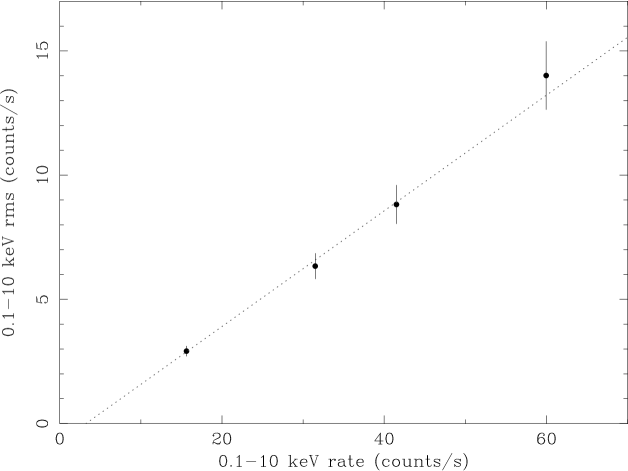
Figure 14: rms-flux relationship for NGC 4051 derived from the XMM-Newton observations in the 0.1-10 keV band. Note the strong linear relationship and the small offset on the flux axis indicating that there is a small component of constant rms. The grey dotted line shows the best-fitting model described in the text.

Figure 15: The Cross Correlation Function of the $0.1-0.5$ light curve vs the $0.5-2$ keV (short-dashed line), the $2-5$ keV (long-dashed line) and the $5-10$ keV (short-long dashed line) lightcurves. The solid line shows the Auto Correlation Function of the $0.1-0.5$ keV lightcurve. The CCFs are all asymmetric towards positive lags, indicative of complex delays between the hard and soft energy band variations

In order to investigate the relationship between the variations in the different energy bands we first estimated their Cross-Correlation Function (CCF). We used 100 s binned lightcurves, and computed the CCF between the $0.1-0.5$ keV lightcurve and the $0.5-2,2-5,$ and $5-10$ keV band lightcurves.

The CCF at each lag $k$, $CCF(k)$, was computed as follows:

$$CCF(k)=\frac{\sum_{t}(x_{soft}(t)-\bar{x}_{soft})(x_{hard}(t+k)-\bar{x}_{hard})}{N(k)(\sigma^{2}_{soft}\sigma^{2}_{hard})^{1/2}},$$

$$k=0,\pm\Delta t,\ldots$$

.

The summation goes from $t=\Delta t$ to $(N-k)\Delta t$ for $k\geq 0$ and from $t=(1-k)\Delta t$ to $N\Delta t$ for $k<0$ ($\Delta t=100$ sec, and $N$ is the total number of points in the lightcurve), while $N(k)$ is the number of pairs that contribute to the estimation of the CCF at lag $k$. The variances in the above equation are the source variances, i.e. after correction for the experimental variance. Significant correlation at positive lags means that the soft band variations are leading the hard band. All the CCFs were computed up to $k=\pm 10$ ks.

The resulting CCFs are shown in Fig. 15. The solid line curve shows the auto-correlation function (ACF) of the $0.1-0.5$ keV lightcurve. All the CCFs show a strong peak ($CCF_{max}>0.8$) at zero lag. The CCF peak decreases as the energy separation of the light curves increases. However, the CCFs are not symmetric. This can be clearly seen when one compares them with the $0.1-0.5$ keV ACF. The asymmetry is in the sense that the correlation at positive lags is larger than the correlation at the respective negative lags. A broadly similar result is found in RXTE observations of NGC7469 by Nandra and Papadakis (2001). Here in NGC 4051, above a lag $\sim 2$ ks, the $0.1-0.5$ keV lightcurve appears to correlate better with the $0.5-2$ and $2-5$ keV lightcurves than with itself. The asymmetry increases with the energy band of the light curves. The $0.1-0.5$ vs $5-10$ keV CCF shows the strongest asymmetry.

The asymmetry of the CCFs towards positive lags indicates the presence of complex delays of the higher energy band lightcurves with respect to the softest band lightcurve. However, the most sensitive tool for the investigation of energy dependent delays is the phase spectrum, which we consider in the next section.

8 Phase Spectrum Analysis

Apart from the CCF, the correlation structure between two lightcurves can also be characterized by the “cross spectral density” function (or simply cross spectrum), which is defined as the Fourier transform of the cross-covariance function of the two lightcurves. The cross spectrum is a complex number, and its argument is called the “phase spectrum”. This function represents the average value of the phase shift between components with the same frequency in the lightcurves. The corresponding shift in the time domain is given by the phase shift divided by the respective frequency, and is usually called the “time lag” at that frequency (or corresponding period).

We used 5 s binned lightcurves in the $0.1-0.5$, $0.5-2$, $2-10$, and $2-5$ keV energy bands, and 100 s binned $0.1-0.5$ and $5-10$ keV light curves, to calculate the phase spectrum of the higher energy bands with the respect to the softest band (i.e. $0.1-0.5$ keV). We used the smaller bin size (5 s) in order to investigate the existence of phase shifts at the highest possible frequencies. In the case of the $5-10$ keV lightcurves, due to the low count rate, we used a larger bin size (100 s) in order to increase the signal to noise ratio. We calculated the real and imaginary parts of the cross-spectral function, grouped them into period bins of constant width in log space, and estimated the phase spectrum following the method described in Papadakis, Nandra and Kazanas (2001).

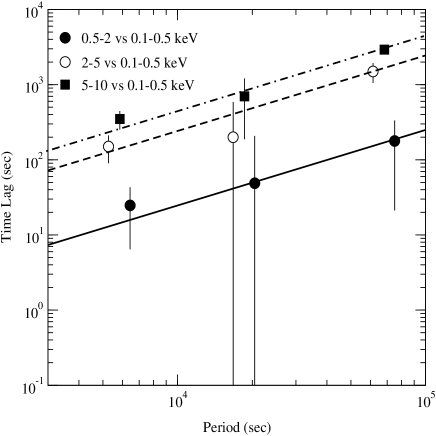
Figure 16: Time lag vs. Fourier period for the cross spectrum of the soft energy band ($0.1-0.5$ keV) vs. the $0.5-2,2-5,$ and $5-10$ keV bands (filled, open circles and filled squares, respectively). The sense of the lag is that the hard bands are all delayed with respect to the soft (0.1-0.5 keV) band. The solid, dashed, and dot-dashed lines show the best-fitting power law model to the respective time lag plots, assuming a slope of 1. Note that the filled black squares are placed in exactly the correct position but the open and filled circles have been displaced slightly to lower and higher periods respectively so that errorbars do not overlap. For any given period the lag increases with the energy separation of the bands.

Our results are shown in Fig. 16. In this figure we show the time lags as function of the Fourier period (i.e., $1/\nu$). For clarity reasons we plot only the lags at the three longest periods, which have the smallest uncertainty. The lags at these periods show clearly that Fourier components in the higher bands are delayed with respect to the same components in the $0.1-0.5$ keV band. The amount of delay does not remain constant but increases with Fourier period. For example, we observe a $\sim 100$ s delay for the components with a period of 5 ks, increasing to $\sim 1$ ks delay for components with a period of 60 ks. This result is similar to the that seen in other Seyfert galaxies (eg NGC 7469, Papadakis et al. 2001; MCG 6-30-15, Vaughan et al. 2003).

We fitted a power-law model of the form, $TimeLag\propto\nu^{-s}$, to the time lags shown in Fig. 16. The best fitting slopes were all consistent with the $s=-1$ value that is commonly found in the time lag plots of GBHs (e.g. Nowak et al. 1999). Therefore as there are few data points and the slope errors are large, we fix the slopes in Fig. 16 at $s=-1$. We see that, at all periods, the lag increases as the separation of the bands increases, from approximately 0.006% of the Fourier period for the $0.1-0.5/0.5-2$ keV lags, to 0.5% of the Fourier period for the $0.1-0.5/5-10$ keV lags.

These results are similar to those observed previously in GBHs (e.g. Nowak et al. 1999) and in MCG-6-30-15 (Vaughan et al. 2003). The increase in lag with both energy separation of the bands and with increasing Fourier period also explains the asymmetric CCFs (Fig. 15).

9 Estimation of the Coherence Function

Having computed the complex cross spectra of the various energy bands, we also estimated their coherence functions. The value of the coherence function between two lightcurves, at a certain frequency, may be interpreted as the correlation coefficient between the Fourier components of the two lightcurves at that frequency,(Priestley 1981; Vaughan and Nowak 1997). If the coherence function is close to unity at all frequencies, we expect to obtain a close linear relationship between the two lightcurves.

Following Papadakis et al. (2001) we computed the coherence functions of the $0.1-0.5/0.5-2$ keV and the $0.1-0.5/2-10$ keV lightcurves. We chose these broad bands to obtain good S/N. Our results are shown in Fig. 17. Although the coherence of both functions is close to unity at the largest periods ($\sim 10^{5}$ s), it decreases as the Fourier period decreases and as the energy separation between the bands increases. This result is similar to that seen in GBHs (eg Nowak et al. 1999) and recently in other Seyfert galaxies (MCG-6-30-15, Vaughan et al. 2003; Mkn 766, Vaughan et al. 2003).

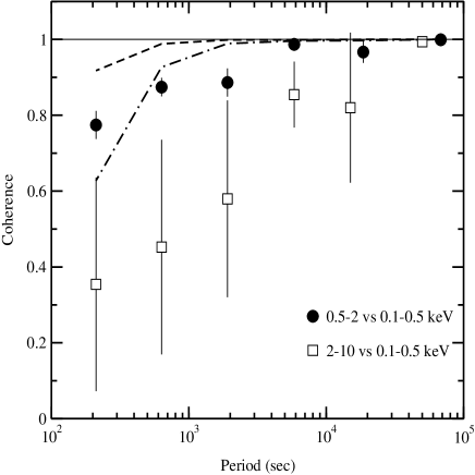
Figure 17: Coherence function vs. Fourier period for the soft energy band ($0.1-0.5$ keV) vs. the $0.5-2$ and $2-10$ keV bands (filled circles and open squares, respectively). Note that, for the $0.1-0.5$ keV vs $2-10$ keV function, the two open squares at the longest Fourier period have been displaced to slightly shorter period to avoid overlapping of their errorbars with the points of the $0.1-0.5$ keV vs $0.5-2$ keV function, which remain in their correct positions. Coherence of unity is indicated by the continuous solid line. The dashed and dot-dashed lines show, for the $0.1-0.5$ keV vs. $0.5-2$ and $2-10$ keV bands respectively, the 95% confidence limit for spurious lack of coherence introduced by the approximation in the numerical calculation. We note that, at shorter Fourier periods, there is a genuine decrease in coherence beyond that introduced by numerical approximation.

The coherence function was corrected for the effects of Poisson noise, and errors were calculated, using Equation 8 of Vaughan & Nowak 1997, which applies in the limit of high PSD power, relative to the Poisson noise level, and high measured coherence. However the high power assumption breaks down at short timescales so, in order to test whether any of the observed drop in coherence is real, we carried out Monte Carlo simulations. We simulated lightcurves with 5 s time resolution and identical duration to the XMM-Newton light curves, choosing underlying PSD models for each band to match the corresponding best fitting constant $\nu_{B}$ model (see Section 5.4). We simulated 200 pairs of light curves for each of the coherence function measurements, forcing the lightcurves to be perfectly correlated (unity coherence) by using the same random number sequence to generate both lightcurves. We then approximated the effects of Poisson noise by adding a random Gaussian deviate to each data point with variance equal to the average squared error of the lightcurve. Coherence measurements were made for each of the 200 lightcurve pairs, and the 95% lower limit on the coherence in each bin is plotted in Fig. 17. The simulations clearly show that although the coherence does drop artificially on short time-scales, the observed drop in coherence is much larger than expected from this effect alone. Therefore most of the observed drop in coherence is intrinsic to the underlying light curves.

10 Summary of Observational Results

In this Section we summarise the main observational results of this paper. In the next Section (§ 11) we discuss the implications of these results.

1. We present $>6.5$ years of well sampled X-ray observations of NGC 4051 by RXTE, together with $\sim 100$ ks of continuous observations with XMM-Newton. The resulting PSD spans over 6.5 decades of frequency and is the best determined AGN PSD yet published.

2. A gently bending powerlaw model is a better fit to the combined RXTE and XMM-Newton PSD of NGC 4051, although a sharply broken powerlaw is still an acceptable fit. The gently bending model is also a much better fit to the high S/N high state PSD of Cyg X-1 than a sharply broken powerlaw. As a gentle bend is also more plausible physically than a sharp break, we use it as our standard description of the PSDs of NGC 4051.

3. The combined RXTE and XMM-Newton (4-10 keV) PSD has a slope, $\alpha_{L}$, of $\sim-1.1$ at low frequencies and steepens, above a break frequency, $\nu_{B}$, of $8\times 10^{-4}$Hz, to a slope, $\alpha_{H}$, of $\sim-2$. There is no evidence of a second break at lower frequencies.

4. In NGC 4051 $\nu_{B}$ is almost independent of energy, as in Cyg X-1 in the high state.

5. In NGC 4051 $\alpha_{H}$ is steeper at lower energies ($\sim-3$, 0.1-2 keV; $\sim-2$, 2-10 keV) whereas in Cyg X-1 in the high state $\alpha_{H}\sim-3$ over all of the presently observable spectral range (2-13 keV).

6. NGC 4051 shows the same rms-flux relationship (Uttley and M^cHardy 2001) which is displayed by GBHs, including the presence of small component of constant rms.

7. As shown by the cross-correlation analysis (Fig. 15), variations in different energy bands are very well correlated in NGC 4051. However as the phase-spectral analysis shows (Fig. 16), there are complex lags between bands, with the hard photons always lagging the soft photons. The lag is greatest for variations of large Fourier period, and also increases as the energy separation between bands increases.

8. The coherence between wavebands is very high at long Fourier periods but decreases at shorter periods, and with increasing separation between wavebands. We note that the decrease in coherence becomes noticeable at the same timescale as the break timescale in the PSD.

11 Implications

11.1 NGC 4051 and Cygnus X-1: A valid comparison?

In the soft high state, the energy spectrum of Cygnus X-1 is dominated by relatively constant thermal emission from the accretion disc below about 6 keV. Above that energy the spectrum is dominated by a variable component of hard spectrum. However in the case of NGC 4051 the constant soft component accounts for only $\sim 10\%$ ($\sim 2$ counts s^-1) of the average flux in the 0.1-0.5 keV band and probably for a similar fraction in the 0.5-2 keV band (cf Uttley et al. 2003). So is it legitimate to compare the PSDs of Cygnux X-1 and NGC 4051 in bands below 6 keV?

In the case of NGC4051 the spectrum below 2 keV is not a simple powerlaw. The complex shape during the present observations is described by Salvi (2003) and Salvi et al. (2003). The rather similar spectral shape during an X-ray low state Targe of Opportunity (TOO) observation by XMM-Newton, triggered as a result of our RXTE monitoring, is reported by Uttley et al. (2003). The spectral shape can be parameterised by a combination of a powerlaw and Comptonised thermal component. However whatever its exact description, the whole continuum from 0.1 to 10 keV, apart from a $\sim 10\%$ constant component, varies together and is consistent with simple spectral pivoting about some high energy (Uttley et al. 2003). The TOO observations are thus entirely consistent with the earlier RXTE and EUVE observations which showed strongly correlated variability in the X-ray and EUV bands. Thus, whatever band we sample in NGC4051, we are sampling overwhelmingly the rapidly variable component.

In the case of Cygnus X-1 in the soft high state, a detailed examination of its variability as a function of energy, has been carried out by Churazov et al. (2001). They show that the soft component is relatively quiescent and that the hard component is responsible for the vast majority of the variability in all bands which they sample (ie above 2 keV). The only effect of the constant soft component on the PSD is to reduce its normalisation as one moves to lower energies where the soft component is more dominant. Indeed Churazov et al. show (their Figure 2) a 6-13 keV PSD which is very similar to that which we show in Fig. 4 and they note that, at lower energies, the normalisation is lower but the shape of the PSD is the same.

Therefore, as far as we are able to determine, over all of the energy ranges discussed in this paper, it is entirely valid to compare the shapes of the PSDs of Cygnus X-1 and in NGC 4051. We do, of course, have to bear in mind the contribution from the constant components when comparing the normalisations of the PSDs.

11.2 NGC 4051: High or Low State System?

The overall long and short timescale PSD of NGC 4051 (Fig. 12) is a very close match to the PSD of Cyg X-1 in a high state (Fig. 4), having the same slopes above and below the break, and with the slope below the break remaining unchanged for over 4 decades. It does not look at all like the PSD of Cyg X-1 in a low state. We therefore conclude that NGC 4051 is the analogue of a GBH in a high state. This is the first definite confirmation of an AGN in a high state.

As an alternative representation we plot, in Fig. 18, the combined RXTE and XMM-Newton (0.1-2 keV) PSD of NGC 4051 in units of frequency $\times$ power ($\nu P_{\nu}$), rather than in units of power. A flat PSD in these units has equal power in every decade of frequency and so this representation is becoming more common as it gives a better idea of the power distribution. In Fig. 18, we show the PSD after it has been unfolded from the model fit to the data. It is the equivalent of an energy spectrum once it has been deconvolved from the instrumental response. Thus although the shape of the PSD in Fig. 18 does depend on the assumed model, it is the closest representation which we can make to the underlying true PSD. We plot similar PSDs for Cyg X-1 in its high and low state. We again note the similarity between the PSD of NGC 4051 and that of Cyg X-1 in its high state. In particular the drop off in power at low frequencies which is apparent in Cyg X-1 in its low state is not seen in the PSD of NGC 4051.

For comparison we also plot the unfolded PSD of the higher mass AGN NGC 3516 (from Uttley et al. 2002). The relative scaling of frequencies with mass is seen quite easily in this figure but we carry out a more quantitative comparison in Section 11.5.

We also note that NGC 4051 has a particularly high variability power and that Cyg X-1, in the high state, is somewhat lower. However we should regard these normalisations with caution as the PSDs have been normalised by the square of the mean flux. Thus any relatively constant soft component, such as contributes to the spectrum of Cyg X-1 in the high state up to $\sim 6$keV, raises the mean flux but does not contribute to the variability.

Figure 18: Unfolded PSDs of NGC 4051 (filled circles), NGC 3516 (open squares) and Cyg X-1 in its low (filled triangles) and high (asterisks) state. Note that, unlike the other PSDs in this paper, we show here frequency $\times$ power, not simply power.

11.3 NGC 4051 Black Hole Mass and Eddington Luminosity

Assuming the bending powerlaw high state model then, assuming a mass of $10M_{\odot}$ for the black hole in Cyg X-1 (Hererro et al. 1995) and a linear scaling of mass with break timescale, we estimate a black hole mass for NGC 4051 of $\sim 3^{+2}_{-1}\times 10^{5}M_{\odot}$ (assuming a sharply breaking powerlaw implies a mass of $\sim 2\times 10^{5}M_{\odot}$.) This (bending powerlaw model) estimated mass is consistent with the recent reverberation determination of $5^{+6}_{-3}\times 10^{5}M_{\odot}$ (Shemmer et al. 2003) and the earlier determination of $1.0^{+1}_{-0.5}\times 10^{6}M_{\odot}$ (Peterson et al. 2000).

For the estimated mass, the Eddington luminosity, $L_{Edd}$, is $\sim 3\times 10^{43}$ ergs s^-1. Taking an average long term 2-10 keV flux for NGC 4051 of $3\times 10^{-11}$ ergs cm^-2 s^-1 , we calculate a luminosity of $\sim 3\times 10^{41}$ ergs s^-1. Assuming an X-ray to bolometric conversion factor of 27 (Elvis et al. 1994; Padovani and Rafanelli 1988), we deduce that NGC 4051 typically radiates at $\sim 30\%$ of $L_{Edd}$. There is a slight caution that, for NLS1s such as NGC4051, more of the accretion power may be radiated in the X-rays than for broad line AGN. However the broad band SED of NGC 4051 presented by Done et al. (1990) is not too different from the SEDs of typical broad line QSOs (cf Fig. 10 of Elvis et al. 1994), with the UV/EUV band still being the dominant band. So although the bolometric correction from the X-ray may not be 27 for NGC 4051, it is still likely to be quite high. Barring better information we continue to assume a value of 27 but we note the uncertainty. Such a high accretion rate compares with typical values of $\leq 8\%$ for GBHs when in a low state or $\mathrel{\hbox{\hbox to0.0pt{\hbox{\lower 4.0pt\hbox{$\sim$}}\hss}\hbox{$>$}}}20\%$ when in the high state (Esin, McClintock and Narayan 1997) and so strengthens the analogy of NGC 4051 with a high state GBH. Apart from the NLS1s, most other Seyfert galaxies radiate at less than 10% of their Eddington luminosity (eg Woo and Urry, 2002) and so might therefore be analogues of low state GBHs.

11.4 The Geometry of the Emission Region

Here we try and place the observational results into some sort of physical framework. We make the underlying assumption that the X-ray emission is produced by Comptonisation of low energy seed photons by energetic electrons in a corona. Before discussing any specific model we make a number of generic points.

11.4.1 Physical Interpretation of the Break Timescale

When considering what physical process the break timescale ($1/8\times 10^{-4}=1250s$) might correspond to, a useful compilation of dynamical, thermal, sound-crossing and viscous timescales is given by Treves, Maraschi and Abramowicz (1988). For a black hole mass of $3\times 10^{5}\rm M_{\odot}$, that timescale corresponds to the dynamical timescale, $T_{dyn}$, at $26R_{G}$ (ie $26GM/c^{2}$). The thermal timescale, $T_{therm}\simeq T_{dyn}/\alpha$, where $\alpha$ is the viscosity parameter and the viscous timescale, $T_{visc}\simeq T_{therm}\left(\frac{R}{H(R)}\right)^{2}$, where $H(R)$ is the scale height of the disc at radius $R$. The value of $\alpha$ is unknown, but probably significantly less than unity. If $\alpha<0.1$, then $T_{therm}>10T_{dyn}$, and 1250s could correspond to the thermal time scale at the innermost part of the disc. In a conventional thin disc, $R>>H(R)$ so that $T_{visc}$, at a given radius, would be much larger than $T_{dyn}$. However in the inner disc $H(R)$ may approach $R$, and $T_{visc}\sim T_{therm}$. Thus 1250s might correspond to the viscous or thermal timescales at $\sim$few $R_{G}$.

11.4.2 PSDs and shot timescale distribution functions

Almost any PSD shape can be produced by ‘shots’ with a suitably chosen distribution of shot timescales (eg Lehto, M^cHardy and Abraham 1991). Breaks (ie smooth bends) in the PSD are associated with breaks or cut-offs in the distribution function. The PSD slope below the break is related to the slope of the distribution function and the slope above the break reflects the shape of the individual shots (eg exponential shots produce a $\nu^{-2}$ PSD). As long as the distribution function is the same for shots producing photons of differing energies, we would expect the PSD below the break to be independent of photon energy. To produce different PSD slopes above the break at different photon energies, we require either that the shots have an energy-dependent shape or that the underlying distribution function does not stop abruptly at some particular timescale, but that it has a longer tail to short timescales at higher energies.

11.4.3 Difficulties with Shot Models

Shot distribution models can produce PSDs which look rather like the original long and short timescale PSD of NGC 5506 (M^cHardy 1989), and like the PSDs described here. However randomly timed shots do not produce the linear rms-flux relationship which is seen in GBHs and AGN (Uttley and M^cHardy 2001), and which is followed closely here by NGC 4051. Some relationship between variations at long and short timescales is required to produce a linear rms-flux relationship. A plausible framework for the rms-flux relationship is provided by the disc model of Lyubarskii (1997) where successively shorter timescales are associated with annuli successively closer to the black hole. A disturbance, perhaps in accretion rate, starts at the outer edge of the disc and propagates in, thus providing the required link between variations at long and short timescales.

11.4.4 Variations from the seed photons or corona?

If the corona is uniform, the flatter PSD slope above the break at high energies cannot be explained if all of the variations come from the seed photons. In that case, the increased scatterings necessary to raise seed photons up to the higher X-ray energies would tend to wash out high frequency variability at high energies, the opposite of what we see. Thus either the corona is not of uniform temperature, or fluctuations within the corona must be responsible for introducing at least some, and possibly most, of the variability at high frequencies.

11.4.5 The Churazov et al. and Kotov et al. Models

By geometrically varying parameters such as the temperature or density of the emitting region, we can preferentially associate different photon energies with different radial locations. If we also associate different variability timescales with different locations we can build models to attempt to explain the variability of GBHs (eg Hua, Kazanas and Cui 1999) and AGN (Papadakis et al. 2001).

Recently Churazov et al. (2001), with later enhancements by Kotov et al. (2001), have built a qualitative geometric model which can explain many of the observational results presented here (cf Vaughan et al. 2003). In the Kotov model a $1/\nu$ powerspectrum of variations, produced at different radii in the accretion flow (Lyubarskii 1997), propagates inwards in an optically thin corona, over the surface of the disc until it hits the X-ray emitting region, whose emission it modulates. Kotov et al. assume that higher energies and shorter timescales are associated together at smaller radii. (One might, perhaps, associate that region with the region where soft seed photons from the disc become plentiful.) The break frequency is associated with a ‘characteristic timescale’ which is, perhaps, the viscous timescale at the edge of the X-ray emitting region.

Flattening of the PSD at high frequencies:  A geometry where shorter timescales and higher energies are associated together at small radii provides an immediate explanation of the flattening of the high, relative to the low, energy PSD at high frequencies.

Decrease of Coherence at Short Fourier Periods:  If the highest energies are preferentially produced at the innermost radii, then the very highest energies see the largest spectrum of variations, including those at the shortest periods. However if the perturbations only propagate inwards (as expected if they are perturbations in accretion rate or, for acoustic perturbations, as a consequence of increasing viscous timescale with increasing radius) then the lower energies do not see the shortest period variations and the coherence decreases as we go to shorter periods and greater separation of the bands.

Zero lag, asymetric, CCFs:  As the bulk of the X-rays will be produced, in all bands, close to the black hole (eg Fabian et al. 2002 require a highly centrally peaked emission profile in the disc to explain the shape of the iron line in MCG-6-30-15) we do not expect large lags between bands on short Fourier timescales and we expect the CCFs between bands, although asymetric, to be peaked at zero lag.

Period Dependent Lags:  However as there will be a larger component of low energy emission produced further out in the disc where longer variability timescales apply we expect increased lags at longer Fourier periods and as the separation of the bands increases. Any dispersion, whereby lower frequencies propagate more slowly inwards towards the main X-ray emitting region, would also lead to period dependent lags.

Small Differences between NGC 4051 and Cyg X-1:  The analogy between NGC 4051 and Cyg X-1 in the high state is not absolutely perfect. Although we do not sample a great deal of the high state PSD of Cyg X-1 above the break, $\alpha_{H}$ appears to be constant with increasing energy, or maybe even steepens, contrary to the behaviour of NGC 4051. The reason for this small difference is not clear, although we may speculate. We associate the broad similarities in the PSDs (ie many decades of slope -1 followed by a break to a steeper slope at a frequency which is energy-independent) with broad similarities in the process which gives rise to the variations. We have described that process above in terms of variations propogating inwards over the accretion disc and eventually modulating the emission from an inner X-ray emitting region. The smaller differences, ie different behaviour of the high frequency PSD, may reflect small differences in the detailed structure of the accretion disc, or emitting corona, which may be caused by differences in accretion rate or temperature of the disc.

For example we discuss above how a geometry where shorter timescales and higher energies are associated together at small radii provides an explanation of the flattening of the high, relative to the low, energy PSD at high frequencies. However if we can contrive that all energies are emitted in the same proportion at all radii, then we expect no change of PSD shape with energy. Such a scenario might result from a more conducting disc with less of a radial temperature gradient.

11.5 Break Timescales for Broad and Narrow Line Seyfert Galaxies

In Fig. 19 we plot the break timescales vs. black hole mass for Cyg X-1, in its high-soft (H) and low-hard (L) states, and for AGN for which break timescales have so far been measured. Narrow line Seyfert 1 galaxies (NLS1s) are shown as open circles and broad line Seyferts as filled circles. The data for Fig. 19, together with relevant references, are given in Table 10. Note that some of the break timescale in Table 10 were derived from a combination of RXTE and XMM-Newton or Chandra observations and so depend to some extent on the assumption that $\nu_{B}$ is independent of energy. The evidence so far (eg Sections 5.4 and 5.5) indicates that this assumption is good but this caveat should be born in mind.

All break timescales refer to the break in the PSD between a low frequency slope of $\sim-1$ and a high frequency slope of $\sim-2$. In the context of a low state model, we therefore refer to the higher of the two PSD break frequencies which, in the case of Cyg X-1, has an average value of 3.3 Hz (Uttley et al. 2002). For Akn 564 we take the break frequency from Papadakis et al. (2002) rather than that from Markowitz et al. as the Papadakis et al. break refers to the break between slopes of -1 and -2 whereas the Markowitz et al. break refers to a break between slopes of 0 and -1. Note that the masses of MCG-6-30-15, Akn 564 and Mkn 766 are not well known (cf Wandel 2002). We therefore do not attempt to place error bars on these masses, except for the upper limit on the mass of Akn 564, from Collier et al. (2001). As the break frequencies derived from smoothly bending models tend to be higher than those derived from sharply breaking models (eg 22 and 13.9 Hz respectively for Cyg X-1, this paper; 1.3 and 1.0$\times 10^{-4}$Hz for MCG-6-30-15, Vaughan et al. 2003) we use the break timescales from the sharply breaking model, as that has been more widely used in the past. When fitting to the combined RXTE and XMM-Newton 4-10 keV data for NGC 4051 we find values of 8 and 2.4$\times 10^{-4}$Hz respectively, although the latter value is not well constrained. When fitting to the RXTE and XMM-Newton 0.1-2 keV data the respective values are 8.0 and 6.1$\times 10^{-4}$Hz. As the ratio of the latter values is similar to that for MCG-6-30-15 we choose, somewhat arbitrarily, to use the timescale associated with 6.1$\times 10^{-4}$Hz.

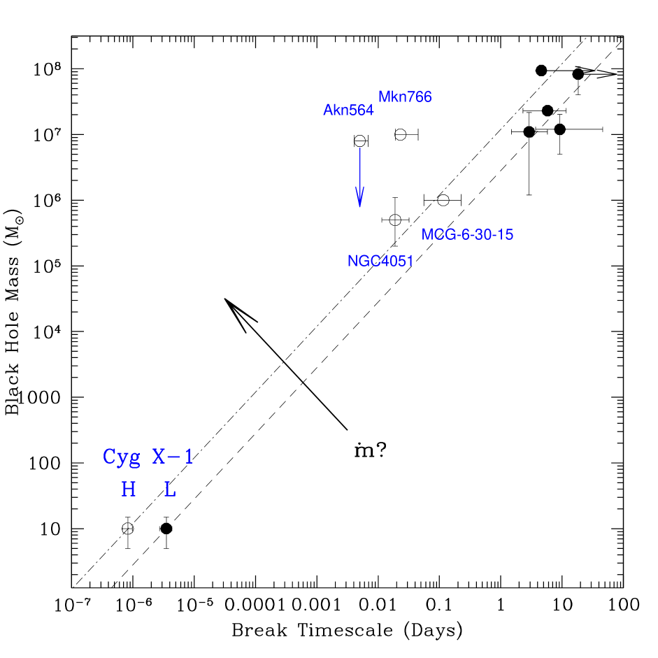
Figure 19: Summary of current PSD break timescales for AGN of various black hole masses. NLS1s are shown as open circles and broad line Seyferts are shown as filled circles. The high-soft (H) and low-hard (L) states of Cyg X-1 are also plotted and lines (dot-dash and long-dash respectively) of slope 1.0 are drawn through those points. The solid arrow labelled with $\dot{m}$ indicates the way that the break timescale/mass line may move with increasing accretion rate. All break timescales refer to a break where the PSD slope below the break frequency is $\sim-1$. All break timescales are derived on the basis of a sharply broken powerlaw model. See text and Table 10 for details.

Table 10: Black Hole Masses and Break Timescales

Target	PSD Break	Ref	BH Mass	Ref
	Timescale (days)		$(10^{7}\,M_{\odot}$)
Fairall 9	$>18.3$	M	$8.3^{+2.5}_{-4.3}$	K
NGC 5548	$>4.6$	M	$9.4^{+1.7}_{-1.4}$	K
Akn 564	$5.0^{+1.8}_{-1.0}\times 10^{-3}$	P	$<0.8$	C
NGC 3783	$2.9^{+2.9}_{-1.4}$	M	$1.1^{+1.1}_{-1.0}$	K
NGC 3516	$5.8^{+5.8}_{-3.5}$	E	$2.3^{+0.3}_{-0.3}$	W
MCG-6-30-15	$1.16^{+1.1}_{-0.6}\times 10^{-1}$	V,U	$\sim 0.1$	M
NGC 4151	$9.2^{+37}_{-5.5}$	M	$1.2^{+0.8}_{-0.7}$	K
NGC 4051	$1.89^{+1.3}_{-0.7}\times 10^{-2}$	T	$5^{+6}_{-3}\times 10^{-2}$	S
Mkn 766	$2.3^{+2.2}_{-0.4}\times 10^{-2}$	VF	$\sim 1.0$	W
Cyg X-1 Low	$3.51^{+0.8}_{-0.8}\times 10^{-6}$	N,U	$\sim 1\times 10^{-6}$	H
Cyg X-1 High	$8.26^{+1.5}_{-1.5}\times 10^{-7}$	T	$\sim 1\times 10^{-6}$	H

REFERENCES:
C - Collier et al. (2001); E - Edelson and Nandra (1999); H - Hererro et al. (1995); K - Kaspi et al. (2000); M - Markowitz et al. (2003); N - Mowak et al. (1999); P - Papadakis et al. (2002); S - Shemmer et al. (2003); T - This work; U - Uttley et al. (2002); V - Vaughan, Fabian and Nandra (2003); VF - Vaughan and Fabian (2003); W - Wandell (2002)

The first point to note from Fig. 19 is that (ignoring the points without good errorbars) the best fit line (not shown, to avoid confusion) through all the AGN has a slope flatter than 1, and does not pass through either of the Cyg X-1 points. No line of slope unity passes through all of the AGN and either one of the Cyg X-1 points. However although it would be something of an exaggeration to say that the timescales associated with broad line AGN scale exactly linearly with mass with that associated with the low state of Cyg X-1, the data are at least consistent with that interpretation. The NLS1s, however, all lie consistently above the low state line and, indeed, almost all lie either on or above the high state line, although note the uncertainties in the masses of 3 of the 4 broad line AGN. The supposition that break timescales, for a given mass, are shorter in NLS1s is strongly supported by the observations of Leighly (1999) who shows that the rms variability of NLS1s is greater than that of broad line galaxies. This result is easily explained if the PSDs of broad line galaxies steepen at lower frequencies than those of NLS1s and so contain less variability power.

The present data indicate that NGC 4051 is radiating at a substantial fraction ($\sim 30\%$) of $L_{Edd}$ and, assuming a high state model, Vaughan et al. (2002) draw a similar conclusion regarding MCG-6-30-15. For Mkn 766 Vaughan and Fabian (2003) note that linear scaling to the high state model implies radiation at greater than $L_{Edd}$, and more serious problems would occur with Akn 564 (cf Papadakis et al. 2002). Scaling the NLS1s to the low state model would make matters much worse.

It should also be noted that although we have shown here that NGC 4051 has a PSD which very closely resembles that of a high state system, we do not yet have such information for Mkn 766 or MCG-6-30-15, although analysis of most recent RXTE data should produce the answer for MCG-6-30-15 (M^cHardy et al. , in preparation).

The PSD of Akn 564 (Papadakis et al. 2002; Pounds et al. 2001) appears to flatten to a slope of zero at the lowest measured frequencies. It could, therefore, be a low state system. However, if so, the mass implied by scaling its break frequency would be extremely low and would imply that Akn 564 was greatly exceeding $L_{Edd}$. An alternative hypothesis is that Akn 564 is the analogue of a very high state system (eg GS 1124-68; van der Klis 1995; McClintock and Remillard 2003). The PSDs of very high state systems, although of variable shape, sometime have the same shape as those of low state systems, but shifted to higher frequencies. Therefore if we were to add another line into Fig. 19 to represent very high state systems, that line would lie above the line of the high state systems.

We therefore hypothesise that the black hole mass/break timescale relationship is not represented by a single relationship for all AGN, but consists of a family of relationships, moving to shorter timescales as some underlying parameter (or possibly more than one parameter) which we have to alter to move from low to very high state systems changes.

In galactic systems it is generally believed (eg Esin et al. 1997; McClintock and Remillard 2003, Homan et al. 2001) that the inner edge of the accretion disc moves closer to the black hole as systems change from the low to the high state. If the break timescale is associated with the edge of the accretion disc, and the same physics (eg viscosity) defines the characteristic timescale in all black hole systems, then movement of the edge of the disc provides a natural explanation of Fig. 19. The main question then would be, what parameter affects the location of the inner edge of the disc? An obvious possibility would be the accretion rate, $\dot{m}$ (eg McClintock and Remillard 2003). That possibility may apply as long as the location of the inner edge of the disc is not restricted by the last stable orbit, ie as long as the inner edge of the optically thick disc remained outside of the last stable orbit. However Homan et al. (2001) suggest that state transitions in the GBH XTE J1550-564 do not depend greatly on $\dot{m}$.

Alternatively, if the discs in all AGN reach right down to the last stable orbit, then we have to alter the location of the last stable orbit and the last stable orbit is closer in for black holes of higher spin (cf Vaughan and Fabian 2003). Thus although it is not possible, on the timescales on which changes are seen, to alter the spin of an individual GBH (or AGN) in order to change it from a low to a high state system, it is possible that, for an ensemble of AGN, a range of spin might provide for a distribution in the mass/break-timescale plane. In either case, AGN which lie above the dot-dash line in the Fig. 19 should have broader X-ray iron emission lines than those lying below the long-dash line. Further observations are required to determine break timescales for a much larger sample of AGN, with a variety of properties, in order to determine which parameters are most important for determining the location of AGN in the break timescale/black hole mass plane.

ACKNOWLEDGEMENTS

We thank the RXTE operations team for their great efforts in scheduling and carrying out the very many observations presented here. We thank the anonymous referee for a very careful and very rapid response. We also thank Chris Done for expert assistance with QDP. This work was supported by grants from the UK Particle Physics and Astronomy Research Council (PPARC) including PPA/G/S/2000/00085. IM^cH also acknowledges the support of a PPARC Senior Research Fellowship.

References

- [] Collier S. et al. 2001, ApJ, 561, 146
- [] Churazov E., Gilfanov M., Revnivtsev M., 2001, MNRAS, 321, 759
- [] Cui W., Zhang S.N., Focke W. Swank J.H., 1997a, ApJ, 484, 383
- [] Cui W., Heindl W.A., Rothschild R.E., Zhang S.N., Jahoda K. Focke W., 1997b, ApJ, 474, L57
- [] Done, C., Ward, M.J., Fabian, A.C., Kunieda, H., Tsuruta, S., Lawrence, A., Smith, M.G., Wamstecker, W., 1990, MNRAS, 243, 713
- [] Done C., Madejski G.M., Mushotzky R.F., Turner T.J., Koyama K. Kunieda H., 1992, ApJ, 400, 138
- [] Edelson R. Nandra K., 1999, ApJ, 514, 682
- [] Edelson R., Turner T.J., Pounds K., Vaughan S., Markowitz A., Marshall H., Dobbie P., Warwick R., 2002, ApJ, 568, 610
- [] Elvis M., Lockman F.J. Wilkes B.J., 1989. Astron. J., 97, 777
- [] Elvis M., Wilkes B.J. McDowell J.C., Green R.F., Bechtold J., Willner S.P., Oey M.S., Polomski E. Cutri, R., 1994, ApJS, 95, 1.
- [] Esin A.A., McClintock J.E. Narayan R., 1997, ApJ, 489, 865
- [] Fabian A.C., Vaughan S., Nandra K., Iwasawa K., Ballantyne D.R., Lee J.L., de Rosa A., Turner A., Young A.J., 2002, MNRAS, 335, L1
- [] Green, A.R., McHardy I.M., Lehto, H.J., 1993, MNRAS, 265, 664
- [] Guainazzi M., et al. 1998, MNRAS, 301, 1.
- [] Hererro A., Kudritzki R.P., Gabler R., Vilchez J.M., Gabler A., 1995, A&A, 297, 556
- [] Homan J., Wijnands R., van der Klis M., Belloni T., van Paradijs J., Klein-Wolt M., Fender, R. Mendez, M., 2001, ApJS, 132, 377
- [] Hua X.-M., Kazanas D. Cui W., 1999, ApJ, 512, 793
- [] Kaspi S., et al. 2002, ApJ, 574, 643
- [] Kotov O., Churazov E., Gilfanov M., 2001, MNRAS, 327, 799
- [] Lamer G., McHardy I.M., Uttley P., Jahoda K., 2003a, MNRAS, 338, 323
- [] Lamer G., Uttley P., McHardy I.M., 2003b, MNRAS, 342, 41L
- [] Lawrence A., Watson M., Pounds K.A. Elvis M., 1987, Nature, 325, 694
- [] Lehto H.J., McHardy I.M. Abraham R.G., 1991, Proc. of Atlanta Conference on Variability of Active Galactic Nuclei, eds Miller H.R., Witta P.J., p256, Cambridge University Press.
- [] Leighly K.M., Mushotzky R.F., Yaqoob T., Kunieda H., Edelson R., 1996, ApJ, 463, 158.
- [] Leighly K.M., 1999, ApJS, 125, 297
- [] Lyubarskii Y.E., 1997, MNRAS, 292, 679
- [] Markowitz, A., Edelson, R., 2001, ApJ, 547, 684
- [] Markowitz, A. et al. , 2003, ApJ, 593, 96
- [] McClintock J.E., Remillard R.A., 2003, astro-ph/0306213
- [] McHardy I.M., 1988, Mem. It. Astr. Soc., 59, 239
- [] McHardy I.M., 1989, ESA SP-296, 1111
- [] McHardy I.M. Czerny, B., 1987, Nature, 325, 696
- [] McHardy I.M., Green A.R., Done C., Puchnarewicz E., Mason K.O., Branduardi-Raymont G., Jones M.H., 1995, MNRAS, 273, 549
- [] McHardy I.M., Papadakis I.E., Uttley P., 1998, Nuc. Phys B, 69, 509
- [] Nandra, K., George I. M., Mushotzky R.F., Turner T. J., Yaqoob T., 1997, ApJ, 476, 70
- [] Nandra, K., Papadakis, I.E., 2001, ApJ, 554, 710
- [] Nowak M.A., Vaughan B.A., Wilms J., Dove J.B., Begelman M.C., 1999, ApJ 510, 874
- [] Ogle, P.M., Mason, K.O., Page, M.J., Salvi, N.J., Cordova, F., McHardy I.M., Priedhorsky, W.C., 2003, ApJ (in press).
- [] Papadakis I.E., Lawrence A., 1993, MNRAS, 261, 612
- [] Papadakis I.E., McHardy I.M., 1995, MNRAS, 273, 923
- [] Papadakis I.E., Nandra K., Kazanas D., 2001, ApJ, 554, 133
- [] Papadakis I.E., Brinkman W., Negoro H. Gliozzi M., 2002, A&A, 382, L1
- [] Padovani P., Rafanelli P., 1988, A&A, 205, 53
- [] Peterson B., et al. , 2000, ApJ, 542, 161
- [] Priestley M.B., 1981, ”Spectral Analysis and Time Series”, Academic Press, London
- [] Pounds K.A., Edelson R.A., Markowitz A., Vaughan S., 2001, ApJ, 550, L15
- [] Reig P., Papadakis. I.E., Kylafis N.D., 2002, A&A, 383, 202
- [] Revnivtsev M., Gilfanov M., Churazov E., 2000, A&A, 363, 1013
- [] Salvi N., 2003, PhD Thesis, University of London
- [] Salvi N., Mason K., Page M. et al. , 2003, MNRAS, in preparation.
- [] Shemmer O., Uttley P., Netzer H., McHardy I.M., 2003, astro-ph/0305129.
- [] Stark A.A., Gammie C.F., Wilson R.W., Bally J., Linke R.A., Heiles C., & Hurwitz M., 1992. Astrophys. J. Suppl., 79, 77
- [] Swank J., 1998, Nuc. Phys. B., 69, 12.
- [] Sunyaev R., Revnivtsev M., 2000, A&A, 358, 617
- [] Taylor, R.D., Uttley, P.U., McHardy I.M., 2003, MNRAS, 242, 31
- [] Timmer J., Konig M., 1995, A&A 300, 707
- [] Treves A., Maraschi L., Abramowicz, M., 1988, PASP, 100, 427
- [] Turner, T.J., George, I.M., Nandra, K., 1998, ApJ, 508, 648
- [] Uttley P., McHardy I.M., Papadakis I.E., Guainazzi M., Fruscione A., 1999, MNRAS, 307, L6
- [] Uttley P., McHardy I.M., Papadakis, I.E., Cagnoni, I., Fruscione, A., 2000, MNRAS, 312, 880.
- [] Uttley P., McHardy I.M., 2001, MNRAS, 323, L26
- [] Uttley P., McHardy I.M., Papadakis I.E., 2002, MNRAS, 332,231
- [] Uttley P., Taylor, R.D., McHardy I.M., Page, M.J., Mason, K.O., Lamer, G., Fruscione, A., 2003, MNRAS (in press).
- [] van der Klis M., 1995, Cambridge Astrophysics Series 26, 252, eds Lewin W.H.G., van Paradijs J., van den Heuvel E.P.J., CUP.
- [] Vaughan B.A., Nowak M.A., 1997, ApJ, 474, L43
- [] Vaughan S., Fabian A.C. Nandra K., 2003, MNRAS, 339, 1237
- [] Vaughan S., Fabian A.C., 2003, MNRAS, 341, 496
- [] Wandel A., 2002, ApJ, 565, 762
- [] Woo J-H., Urry C.M., 2002, ApJ, 579, 530
- [] Zdziarski A.A., Poutanen J., Paciesas W.S., Wen L., 2002, ApJ, 578, 357.
- [] Zhang W., Giles A.B., Jahoda K., Soong Y., Swank J.H. Morgan E.H., 1993, In Siegmund O.H., ed EUV, X-ray and Gamma-ray Instrumentation for Astronomy IV, SPIE, Bellingham WA, p. 324.