An Extremely Young Massive Stellar Object
near IRAS 07029-1215

Abstract

In the course of a comprehensive mm/submm survey of massive star-forming regions, the vicinities of a sample of 47 luminous IRAS sources were closely investigated with SCUBA and IRAM bolometers in order to search for massive protostellar candidates. A particularly interesting object has been found in the surroundings of the bright FIR source IRAS 07029-1215. Follow-up line observations show that the object is cold, that it has a massive envelope, and that it is associated with an energetic molecular outflow. No infrared point source has been detected at its position. Therefore, it is a very good candidate for a member of the long searched-for group of massive protostars.

(catalog IRAS 07029-1215)

1 Introduction

The study of the earliest stages of massive star formation (MSF) is one of the most exciting subjects of present research in this field. Whether the dominant formation process for massive stars is disk accretion (see e.g. Jijina & Adams, 1996) or coalescence (Bonnell, Bate, & Zinnecker, 1998) is still an open question. The presence of outflows in regions of massive star formation favours, however, the first scenario. Similarly to previous surveys (e.g. Beuther et al., 2002, Mueller et al., 2002 or Hunter et al., 2000), we have searched for MSF candidates located near bright IRAS sources using SCUBA and IRAM bolometers (Posselt, 2003 and Klein et al. 2003, in prep.). Our focus was on objects unrelated to the IRAS sources themselves, looking for the earliest evolutionary stages not yet seen in the near- to mid-infrared wavelength regime. Even if we do not yet know what the observational features of massive protostars are (Evans et al., 2002), their invisibility at NIR/MIR wavelengths is a defining criterion. Near IRAS 07029-1215, an object with an IRAS luminosity of $L(IRAS)=1700$ L_⊙ (Henning et al., 1992) at its distance of $d=1$ kpc, we discovered a deeply embedded object (UYSO 1, for Unidentified Young Stellar Object 1), powering a high-velocity bipolar CO outflow. The IRAS source is located in the bright H ii region S 297, illuminated by the B1II/III star HD 53623 (Houk & Smith-Moore, 1988). UYSO 1 is located very close to the edge of a dark cloud.

2 Observations

CO($J=3\to 2$) line mapping of UYSO 1 was carried out with the James Clerk Maxwell Telescope (JCMT) on Mauna Kea, Hawaii, in October 1999. The facility receiver B3 (315-373 GHz) was used as frontend, the Digital Autocorrelation Spectrometer (DAS) as backend. With a total bandwidth of 250 MHz, centered on v${}_{lsr}=+12$ km s^-1, the maps were obtained in position-switch mode with an off-position 10′ to the east. Map sampling was at intervals of 10″, the total on+off integration time was 10 min, the beam efficiency $\eta=0.63$, and the beam size was 14″. Additionally, SCUBA continuum observations at $\lambda=450$ $\mu$m and $\lambda=850$ $\mu$m were performed with a total integration time of 46 minutes. Here, beam sizes were 8″ and 14″, respectively. Based on six different field scans with different chop throws, noise was minimised using the Emerson II technique (Emerson, 1995). In March 2003, additional CS($J=2\to 1$), CS($J=5\to 4$), SiO($J=2\to 1$) and especially H₂CO($J=3_{03}-2_{02}$)/($J=3_{22}-2_{21}$) observations were obtained at the IRAM 30m telescope using the B100, B230, A100 and A230 receivers. The raster map sampling was the same as for the JCMT observations, though a smaller range of offset positions was observed. The center position is shifted southward by 6.4″ when compared to the JCMT map. Data was obtained in position switch mode, integration time at each offset was 6 min. All line observations together with the observing parameters are summarized in Tab. 1.

We used the CLASS software developed by the Grenoble Astrophysics Group for the line data reduction, including zero-order baseline subtraction, and GAIA for the SCUBA data.

3 Results

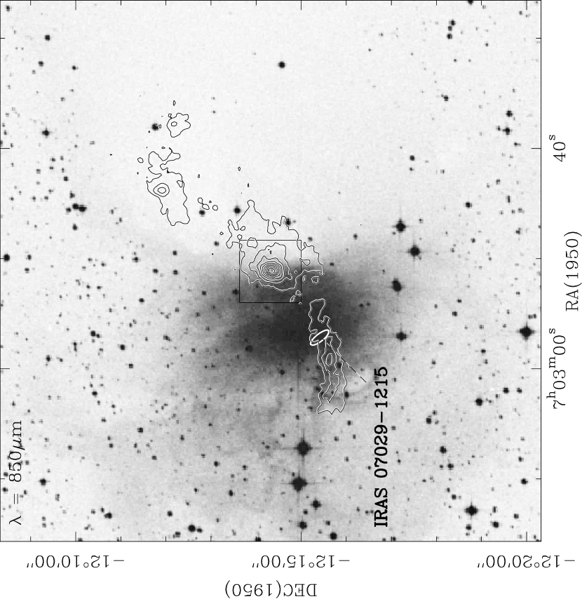
Figure 1: The surroundings of UYSO 1: POSS-I, overlaid with 850 $\mu$m continuum from the JCMT. The box indicates the FOV of Fig. 2.

The POSS view in Fig. 1 shows the environment of IRAS 07029-1215. The overlaid SCUBA map at 850 $\mu$m displays UYSO 1 as a compact emission peak at $\alpha_{\rm(B1950.0)}=07^{\rm h}02^{\rm m}51^{\rm s},\delta_{\rm(B1950.0)}=-12$^∘$14^{\prime}26"$, between S 297 and the dark cloud. In addition to this, two dusty filaments are visible at 850 $\mu$m. The eastern filament contains the IRAS point source position, the western one is located inside the dark cloud.

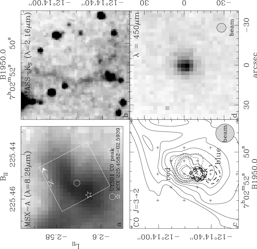
Figure 2: Close-up views of UYSO 1 in a) MSX-$A$, b) 2MASS-$K_{S}$, c) CO($J=3\to 2$) and d) 450 $\mu$m continuum (both JCMT). The box in the MSX data shows the FOV of the other pictures. The integrated CO line data is shown in 10% contours, the two line wings are shown down to 50% intensity. Spectra positions are indicated as well as the beam sizes for CO and the 450 $\mu$m continuum. UYSO 1 is located just below the center position at [0″,-10″], the position of the CO peak.

UYSO 1 is still invisible at near- and mid-infrared wavelengths: No infrared point source in the $\lambda=$2.2..20 $\mu$m range is visible in 2MASS and MSX images (see Fig. 2a,b), but some faint ”reflected” light can be seen in the 2MASS $K_{S}$-band image. It cannot be ruled out, however, that this is captured H₂ line emission, e.g. tracing cloud surfaces and outflows. Neither the IRAS, nor the 2MASS, nor the MSX infrared survey point source catalogues resulted in detections at the UYSO 1 position. There is, however, an MSX point source inside the ”reflected” light south of UYSO 1.

The CO map in Fig. 2c is a close-up view of the dense dust core. The line wings, extending from $-20$ km s^-1 at [0”,-20”] to $+40$ km s^-1 at [0”,0”] (see Fig. 3), can be clearly distinguished from well-determined baselines, extending from $-40$ km s^-1 to $+50$ km s^-1, respectively. Lines are narrower in off-outflow positions. Fig. 4 shows a comparison of the CO($J=3\to 2$) line profile with the CS($J=5\to 4$) profile in the map center. CS($J=5\to 4$) is a high-density tracer with a critical density of n${}_{\rm crit}=7\times 10^{6}$ cm^-3.

Contrary to what could be expected from the 850 $\mu$m map, the CO data do not show a spherically symmetric structure. Instead, the envelope seems to be compressed towards the H ii region east of it. The CO peak is roughly 10″ off the SCUBA peak position. The line wing map displays a bipolar outflow in the NW-SE direction, its origin being UYSO 1 at raster coordinates [0″,-10″], taking the emission peak of the complete integrated line as definition. The outflow is not clearly visible in the CS data, possibly due to the average density being below the CS critical densities. Lines on corresponding positions have, however, corresponding shapes. SiO($J=2\to 1$) could only be detected at the position [-10″, 16.4″], in the outer regions of the redshifted outflow lobe. Possibly, this is due to a bow shock caused by the outflow colliding with the local interstellar medium. The detection at this position is a 6 $\sigma$ detection. With the spatial resolution of the present observations, we cannot decide whether the bipolar outflow is composed of only one or more components (cf. Beuther et al., 2002b).

The SCUBA 450 $\mu$m map (see Fig. 2d) only shows a point source 6″ to the north of UYSO 1, but in between the two outflow lobes.

4 Analysis

From the CO($J=3\to 2$) observations, the object mass and outflow parameters can be deduced. The mass derived from an integration of column densities can be compared to the virial mass. Line wing analysis delivers physical parameters of the bipolar outflow, however still dependent on the unknown outflow inclination angle. The distance to UYSO 1, assumed to be about the same as the distance to IRAS 07029-1215, was kinematically determined to be 1 kpc by Wouterloot & Brand (1989). However, while the distance to the illuminating star of S 297, namely HD 53623, was spectroscopically determined to be 2.2 kpc $\pm$ 25% by Neckel, Klare, & Sarcander (1980), Hipparcos measured a parallax for HD 53623 of $\pi=2.21\pm 1.01$ mas, corresponding to a distance of $450^{+380}_{-140}$ pc (ESA, 1997). Assuming the true distance is near the upper limit of this interval, we adopt a value of 1 kpc for the following mass estimates, in accordance with detailed studies of CMa R1 by Shevchenko et al. (1999) and de Zeeuw, Hoogerwerf, & de Bruijne (1999).

The CO data analysis is depicted in Fig. 2c, in direct comparison to 2MASS-$K_{S}$ data and the 450 $\mu$m continuum.

4.1 Temperature Determination

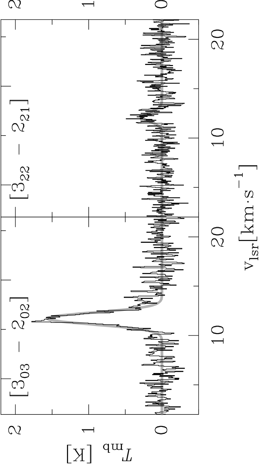
Figure 5: Temperature determination with H₂CO lines (see text). Gaussian fit results are shown in grey.

While the main beam temperatures $T_{\rm mb}$ of the highly optically thick CO lines already confine the kinetic temperature to the 40-50 K range, another estimate was obtained from H₂CO($J=3_{03}\to 2_{02}$)/($J=3_{22}\to 2_{21}$) data, following Mangum & Wootten (1993). Fig. 5 shows the two H₂CO transitions for UYSO 1. The intensity ratio deduced from fitted Gaussians is 6, thus indicating a kinetic temperature of T=40$\pm 5$ K for a relatively wide range of densities.

4.2 Mass Determination

Assuming virial conditions, i.e. assuming that the observed line width is entirely due to motion in gravitational equilibrium, the total mass of the object can be estimated as described by Henning et al. (2000). Inside a sphere of 0.14 pc radius, corresponding to the 40% contour level (deconvolved with the 14″ beam) at 10 $\sigma$, and using the Gaussian fit result of $\Delta v=3$ km s^-1, a virial mass of $M_{\rm vir}=180$ M_⊙ is obtained.

Following Henning et al. (2000), we derive hydrogen column densities from the CO($J=3\to 2$) transition, assuming a relation of $N(\rm H_{2})$ (cm${}^{-2})=3\times 10^{20}\int T_{\rm mb}\rm dv$. An underlying assumption is a conversion factor of CO($J=3\to 2$) / CO($J=1\to 0$) close to unity, as it is frequently observed in massive star-forming regions and explained by clumpy structure (Störzer et al., 2000). The gas mass of the cloud can then be determined as $M_{\rm gas}=2$m${}_{\rm H}\bar{\mu}A\langle N($H${}_{2})\rangle$, where $\bar{\mu}=1.36$ takes into account the interstellar mean molecular weight per H atom. $A$ is the area occupied by the source.

Within the same area and to the same confidence level as the virial analysis, this leads to a different result for the cloud mass. With an average column density of $N$(H₂) = $3.2\times 10^{22}$ cm${}^{-2}\!\!,$ the resulting mass is $M_{\rm gas}=40$ M_⊙.

Another estimate for the total mass has been calculated from the continuum observations at $\lambda=850$ $\mu$m. Assuming a dust temperature of $T_{\rm d}=20$ K and optically thin conditions, $M_{\rm gas}=F_{\nu}\cdot d^{2}/(\kappa_{m}(\nu)\cdot B_{\nu}(T_{\rm d}))\cdot[M_{\rm gas}/M_{\rm dust}]$. Using an interpolated opacity of $\kappa=1.97$ cm^-2/g (thin ice mantles, Ossenkopf & Henning, 1994), the result is $M=15$ M_⊙. The radius of the region taken into account for this calculation is 0.11 pc (at a distance of 1 kpc), slightly smaller than the 0.14 pc used here. Additionally, the dust continuum emission traces only the high-density central regions while the CO emission is collected along the line of sight throughout the low-density halo. Optically thick emission might further influence the estimate (see §4.4). These two points at least partly explain the discrepancy.

Thus, the mass estimates based on line and dust emission are compatible when keeping in mind their respective limitations and range between 15 and 40 M_⊙. The virial mass is much higher which is certainly caused by an overestimation of line width due to optical thickness and turbulent motion, in addition to the cloud not being in virial equilibrium.

4.3 Outflow Properties

The two line wings were analyzed to their respective 10% contour levels, corresponding to a 2 $\sigma$ detection for the redshifted line wing and a 4 $\sigma$ detection for the blueshifted line wing. The masses inside the two outflow lobes are again calculated by integration of H₂ column densities, resulting in $M_{\rm blue}=1.8$ M_⊙ and $M_{\rm red}=3.6$ M_⊙, the total outflow mass thus being $M_{\rm out}=5.4$ M_⊙.

The maximum projected velocities of the red and blue line wings are $v_{\rm proj,r}=27.9$ km s^-1 and $v_{\rm proj,b}=32.1$ km s^-1 respectively, the mean value being $v_{\rm proj}=30$ km s^-1. Together with the known distance and the outflow radial sizes, the dynamical timescale and the mass loss rate can be obtained. With caution, the latter can be empirically converted to luminosity, and spectral type as well as mass of an assumed central star. All values discussed hereafter are summarized in Tab. 2 for inclinations of $i=10^{\circ}\!\!,$ $i=57.3^{\circ}$ (the most probable value, cf. Bontemps, Ward-Thompson, & André, 1996) and $i=80^{\circ}\!\!.$

When the apparent outflow velocity $v_{\rm proj}$ and the apparent maximum outflow extension have been inclination-corrected to $v_{\rm out}$ and $R_{\rm out}$, the dynamical timescale can be calculated from $t_{\rm d}(i)=R_{\rm out}(i)/v_{\rm out}(i)$. The resulting values range from $t_{\rm d}(80^{\circ})\approx 500$ years to $t_{\rm d}(10^{\circ})\approx 1.5\times 10^{4}$ years. However, the timescale estimated this way is not a good age indicator. Only a massive object can uphold mass outflow rates $\dot{M}(i)=M_{\rm out}(i)/t_{\rm d}(i)$ ranging from $\dot{M}(10^{\circ})\approx 4\times 10^{-4}$ M_⊙/yr to $\dot{M}(80^{\circ})\approx 1\times 10^{-2}$ M_⊙/yr. They can be empirically transformed into the luminosity of the central object according to Shepherd & Churchwell (1996), Henning et al. (2000) or, based on a more comprehensive sample, by Beuther et al. (2002b). Tab. 3 summarizes the resulting spectral types, masses and luminosities (using data by Lang, 1991). However, these properties of the central object can be better determined using the SED (see §4.4).

It may be interesting to consider the age of the neighbouring H ii region. Following Cernicharo et al. (1998), this age can be estimated (Whitworth et al., 1994). The size of S 297 in the optical regime with a diameter of 7’ (Sharpless catalogue) corresponds to a radius of only about $2.1\times 10^{5}$ AU, hence indicating that the nebula is rather young. Assuming a typical mean density of $10^{3}$ cm^-3 and a Lyman continuum flux for a B1 star from Thompson (1984), the resulting age is approximately $7\times 10^{5}$ yrs.

Regardless of the uncertainties in these age estimates, the H ii region is likely to be older than UYSO 1. Possibly, this is an example of induced star formation, although this would need kinematic confirmation.

4.4 Spectral Energy Distribution

While the two measured continuum fluxes at 450 $\mu$m and 850 $\mu$m determine the cold dust emission, more data had to be complemented before the spectral energy distribution could be tentatively compared to modeling results. Given the aim of determining the luminosity and mass of the central object as well as having a comparison to the mass determination, upper flux limits for short wavelengths helped pinning down physical properties of the central object. As main support besides the JCMT data, IRAS fluxes were used, determined at the position of UYSO 1 within beam sizes from the IRAS atlas maps. UYSO 1 is unresolved also on IRAS HIRES maps. Additionally, data for the definitely brighter nearby MSX point source G225.4582-02.5939 and 2MASS detection limits set further constraints.

Integrating the SED and using the flux limits at infrared wavelengths as the actual flux values leads to a luminosity of $<1900$ L_⊙, assuming spherical symmetry. A modified blackbody accounting for the dust optical depth was fitted to the data: $S_{\nu}=B_{\nu}(T)(1-\exp(-\tau_{\nu}))\Delta\Omega$, with the beam size $\Delta\Omega$ and with dust opacities $\kappa_{\nu}\propto\nu^{\beta}$ (see e.g. Hildebrand, 1983). A good fit is obtained for $T=45$ K and $\beta=2$, however fits with temperatures between 40 and 50 K are also fitting the data within the uncertainties. With the aim of checking the consistency of existing data, the continuum emission was then modeled using the radiative transfer code developed by Manske, Henning, & Men’shchikov (1998). This is an accelerated version of the 2-D ray-tracing code developed for radiative transfer in disk configurations by Men’shchikov & Henning (1997). Due to insufficient parameter constraints, the code was used in its 1D version only.

The limiting outer radius of the model could be estimated from the CO data to be $3.2\times 10^{4}$ AU, taking the same area as for the mass estimation. Assuming an exponential of the density distribution of 2.0 with a dust-to-gas ratio of 1:150, the model uses silicate optical data from Dorschner et al. (1995), while the properties of the carbonaceous dust are from Jäger et al. (1998) [1000 K data]. The ratio of silicates to carbon is 3:2. The inner model radius is determined by the dust sublimation temperature of 1500 K.

Fig. 6 shows the results for an envelope mass of $M_{\rm env}=30$ M_⊙ and an assumed single central object in the B2.5 class. The optical depth at $\lambda=500$ nm for the simulation runs is $\tau_{500\rm nm}\approx 6400$. Since the code becomes inaccurate for high optical depths, the computed SED is arbitrarily shown for $\tau\lesssim 1000$, corresponding to $\lambda>10$ $\mu$m. At $\lambda=850$ $\mu$m, the optical depth is $\tau_{850\rm\mu m}\approx 1$. Thus, the mass estimate from the dust emission in §4.2 is rather a lower limit because of contribution from optically thick emission.

Both the simulation and the blackbody fit indicate the equivalent of an early B star as the central object. This finding is compatible with the result of the empirical outflow analysis for $i=57.3^{\circ}$. The envelope mass in the simulation is compatible with the mass estimate from the CO($J=3\to 2$) data (40 M_⊙), especially when keeping in mind that the modeled gas density only reaches $10^{4}$ cm^-3 at its outer radius, thus allowing for a slightly higher envelope mass when integrating further outwards.

5 Conclusions

The emerging picture of UYSO 1 drawn from both mass estimates and subsequent empirical relations as well as SED considerations thus is that of an early B star surrounded by an envelope of about 30-40 M_⊙. The object seems to be in a particularly early evolutionary state, but already drives a bipolar outflow with a total mass of M${}_{\rm outflow}=5.4$ M_⊙. To our knowledge, there are only very few comparable sources that are undetected at infrared wavelengths (see e.g. Hunter et al., 1998, Bernard, Dobashi, & Momose, 1999 and Fontani et al., 2003). With additional high-resolution observations, we hope to be able to specify these conclusions and learn more about this evolutionary state. Possibly, parameters of a putative disk around UYSO 1 could be derived then.

Table 1: Heterodyne observations of UYSO 1

Line	Frequency	Telescope	Date	beam size	$\eta_{\rm mb}$
CO($J=3\to 2$)	345.79 GHz	JCMT	Oct 99	14”	0.63
CS($J=2\to 1$)	97.98 GHz	IRAM 30m	Mar 03	25”	0.78
CS($J=5\to 4$)	244.94 GHz	IRAM 30m	Mar 03	10”	0.50
SiO($J=2\to 1$)	86.84 GHz	IRAM 30m	Mar 03	29”	0.78
H2CO($J=3-2$)	218.34 GHz	IRAM 30m	Mar 03	12”	0.56

Table 2: UYSO 1 outflow properties

i	vout	Rout	td	$\dot{\rm{M}}$
$10^{\circ}$	30.5 km s-1	$1.4\times 10^{13}$ km	14600 yrs	$3.7\times 10^{-4}$ M⊙/yr
$57^{\circ}\!\!.3$	55.5 km s-1	$2.9\times 10^{12}$ km	1700 yrs	$3.3\times 10^{-3}$ M⊙/yr
$80^{\circ}$	172.7 km s-1	$2.4\times 10^{12}$ km	450 yrs	$1.2\times 10^{-2}$ M⊙/yr

Table 3: Outflow-inferred properties of assumed central star

i	L	spec. type	Mstar
$10^{\circ}$	$10^{3}$ L⊙	B4	6.5 M⊙
$57^{\circ}\!\!.3$	$10^{4}$ L⊙	B1	13 M⊙
$80^{\circ}$	$10^{5}$ L⊙	O9	19 M⊙

Figure 3: CO($J=3\to 2$) spectra on the inner grid. The line maxima (all between 40 K and 50 K) were cut to allow for a better depiction of line wings.

Figure 4: Comparison of the CO($J=3\to 2$) and CS($J=5\to 4$) lines at the respective peak positions: the CO line at [0″,0″] and an addition of four CS spectra, amplified ten times for depiction, at [0″,-6.4″]. Positions are in arcseconds relative to the center position of the CO grid.

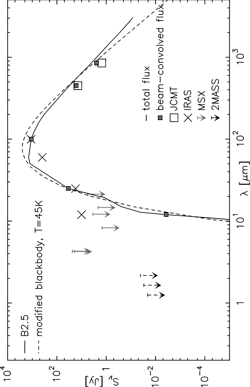
Figure 6: Modeling results from the Manske code. The straight line shows the total flux (displayed for $\tau_{\lambda}\lesssim 1000$), boxes indicate beam-convolved fluxes. The dashed line corresponds to a modified blackbody at T=45 K (with $\beta=2$)

References

- Bernard, Dobashi, & Momose (1999) Bernard, J. P., & Dobashi, K., Momose, M. 1999, A&A, 350, 197
- Beuther et al. (2002) Beuther, H., Schilke, P., Menten, K. M., Motte, F., Sridharan, T. K., & Wyrowski, F. 2002, ApJ, 566, 945
- Beuther et al. (2002b) Beuther, H., Schilke, P., Sridharan, T.K., Menten, K.M., Walmsley, C.M., & Wyrowski, F. 2002, A&A, 383, 892
- Bonnell, Bate, & Zinnecker (1998) Bonnell, I.A., Bate, M.R., & Zinnecker, H. 1998, MNRAS, 298, 93
- Bontemps, Ward-Thompson, & André (1996) Bontemps, S., Ward-Thompson, D., & André, P. 1996, A&A, 314, 477
- Cernicharo et al. (1998) Cernicharo, J., Lefloch, B., Cox, P., Cesarsky, D., Esteban, C., Yusef-Zadeh, F., Méndez, D.I., Acosta-Pulido, J., Garcia López, R.J., & Heras, A. 1998, Science, 282, 462
- de Zeeuw, Hoogerwerf, & de Bruijne (1999) de Zeeuw, P.T., Hoogerwerf, R., & de Bruijne, J.H.J. 1999, AJ 117, 354
- Dorschner et al. (1995) Dorschner, J., Begemann, B., Henning, Th., Jäger, C., & Mutschke, H. 1995, A&A, 300, 503
- Emerson (1995) Emerson, D. T. 1995, in ASP Conf. Ser., Vol. 75, Multi-feed Systems for Radio Telescopes, ed. D. T. Emerson, J. M. Payne, (San Francisco: ASP)
- ESA (1997) ESA 1997, The Hipparcos and Tycho Star Catalogues, ESA SP-1200
- Evans et al. (2002) Evans II, N.J., Shirley, Y.L., Mueller, K.E., & Knez, C. 2002, in ASP Conf.Ser.267, Hot Star Workshop III: The Earliest Phases of Massive Star Birth, ed. P.A. Crowther (San Francisco: ASP)
- Fontani et al. (2003) Fontani, F., Cesaroni, R., Testi, L., Walmsley, C.M., Molinari, E., Neri, R., Shepherd, D., Brand, J., Palla, F., & Zhang, Q., A&A, in press
- Henning et al. (1992) Henning, Th., Cesaroni, R., Walmsley, M., & Pfau, W. 1992, A&AS, 93, 525
- Henning et al. (2000) Henning, Th., Schreyer, K., Launhardt, R., & Burkert, A. 2000, A&A, 353, 211
- Hildebrand (1983) Hildebrand, R.H. 1983, QJRAS, 24, 267
- Houk & Smith-Moore (1988) Houk, N., & Smith-Moore, M. 1988, Michigan catalogue of Two-Dimensional spectral types for the HD stars,vol. 4 : -26 to -12 degrees, Michigan Spectral Survey (Ann Arbor, Dept. of Astronomy, Univ. Michigan)
- Hunter et al. (1998) Hunter, T.R., Neugebauer, G., Benford, D.J., Matthews, K., Lis, D.C., Serabyn, E., & Phillips, T.G. 1998, ApJ, 493, L97
- Hunter et al. (2000) Hunter, T. R., Churchwell, E., Watson, C., Cox, P., Benford, D. J., & Roelfsema, P. R. 2000, AJ, 119, 2711
- Jäger et al. (1998) Jäger, C., Mutschke, H., Dorschner, J., & Henning, Th. 1998, A&A, 332, 291
- Jijina & Adams (1996) Jijina, J., & Adams, F.C. 1996, ApJ, 462, 874
- Lang (1991) Lang, K.R. 1991, Astrophysical Data: Planets and Stars (Berlin: Springer)
- Mangum & Wootten (1993) Mangum, J.G., & Wootten, A. 1993, ApJS, 89, 123
- Manske, Henning, & Men’shchikov (1998) Manske, V., Henning, Th., & Men’shchikov, A.B. 1998, A&A, 331, 52
- Men’shchikov & Henning (1997) Men’shchikov, A. B., & Henning, Th. 1997, A&A, 318, 879
- Mueller et al. (2002) Mueller, K.E., Shirley, Y.L., Evans, N.J., II, & Jacobson, H.R. 2002, ApJS, 143, 469
- Neckel, Klare, & Sarcander (1980) Neckel, Th., Klare, G., & Sarcander, M. 1980, A&ASS, 42, 251
- Ossenkopf & Henning (1994) Ossenkopf, V., & Henning, Th., A&A, 291, 3
- Posselt (2003) Posselt, B. 2003, diploma thesis, Friedrich Schiller University, Jena, Germany
- Rohlfs & Wilson (2000) Rohlfs, K., & Wilson, T.L., 2000, Tools of Radio Astronomy (Berlin: Springer)
- Shepherd & Churchwell (1996) Shepherd, D.S., & Churchwell, E. 1996, ApJ, 472, 225
- Shevchenko et al. (1999) Shevchenko, V.S., Ezhkova, O.V., Ibrahimov, M.A., van den Ancker, M.E., & Tjin A Djie, H.R.E. 1999, MNRAS, 310, 210
- Störzer et al. (2000) Störzer, H., Zielinsky, M., Stutzki, J., & Sternberg, A. 2000, A&A, 358, 682
- Thompson (1984) Thompson, R.I. 1984, ApJ, 283, 165
- Whitworth et al. (1994) Whitworth, A.P., Bhattal, A.S., Chapman, S.J., Disney, M.J., & Turner, J.A. 1994, MNRAS, 268, 291
- Wouterloot & Brand (1989) Wouterloot, J.G.A., & Brand, J. 1989, A&AS, 80, 149