Modeling of Dust Scattering in the Coalsack

Murthy et al. (1994) discovered intense UV (1100 Å) emission from the direction of the Coalsack Nebula. We have used their results in conjunction with a Monte Carlo model for the scattering in the region to show that the scattering is from dust in the foreground of the Coalsack molecular cloud. We have constrained the albedo of the grains to 0.4 $\pm$ 0.1. This is the first determination of the albedo of dust in the diffuse ISM in the FUV.

1 Introduction

Although a potentially useful test of models of interstellar dust grains, measurements of the optical parameters — the albedo ($\it{a}$) and the phase function asymmetry factor ($\it{g}$) — of the grains have been too uncertain to have been of much utility (for a recent review see Draine 2003a). Both methods used to investigate the scattering properties have been problematic: reflection nebulae because an uncertain geometry can heavily influence the derived parameters (Mathis et al. 2002) ; and the diffuse background because of its faintness and because there is often a tradeoff between $a$ and $g$ which allows neither to be tightly constrained (Draine 2003a).

The Coalsack Nebula, one of the most prominent dark nebulae in the Southern Milky Way, offers an excellent location for the determination of the scattering function of the diffuse grains, particularly in the UV where Murthy et al. (1994) found it to be one of the brightest sources of diffuse emission in the sky. Without detailed modeling, they were unable to provide useful contraints on the optical constants of the grains but did suggest that most of the observed emission was due to forward scattering of photons from three of the brightest UV stars in the sky (Table 1) by foreground dust, rather than back-scattering from dust in the molecular cloud. We note that Mattila (1970) observed scattering from the Coalsack in the visible which he interpreted as being due to scattering from the Coalsack.

In this paper, we have reinterpreted the $\it{Voyager}$ observations of Murthy et al. using improved distances for the three stars, a detailed model for the interstellar dust distribution and a Monte Carlo model for the grain scattering. In agreement with Murthy et al., the observed radiation is dominated by scattering from dust in the foreground cloud, rather than the Coalsack molecular cloud. The albedo is tightly constrained to a value of 0.4 $\pm$ 0.1 at 1100 Å.

Table 1: Properties of stars in our model

Name	$\it{l}$	$\it{b}$	distance	flux(1100 Å)
	(deg)	(deg)	(pc)	(photons s-1 Å-1 )
$\alpha$ Cru	300.13	-0.36	98.3	8.86$\times$108
$\beta$ Cru	302.46	3.18	108.1	9.70$\times$108
$\beta$ Cen	311.77	1.25	161.3	2.53$\times$109

2 Model

We have developed a generalized Monte Carlo model to simulate the scattered emission from a star in an arbitrary scattering geometry. Each photon from the star is emitted in a random direction and continues in that direction until an interaction occurs, the probability of which depends on the local dust density. At the point of interaction, we reduce the photon’s effective weight by a factor of $\it{a}$, the grain albedo, and calculate a new direction using the Henyey-Greenstein (Henyey & Greenstein 1941) scattering function:

$$\phi(\theta)=\frac{(1-{\it g}^{2})}{(1+{\it g}^{2}-2{\it g}cos(\theta))^{3/2}}$$ (1)

In Eqn. 1, $\it{g}$ is the phase function asymmetry factor (defined as $\langle cos(\theta)\rangle$) and $\theta$ is the angle of scattering. If g is close to zero, the scattering is nearly isotropic while a value of g near 1 implies strongly forward scattering grains.

We follow the photon through a sequence of interactions until it either leaves the area we are considering or its intensity drops to a negligible value. To save computational time, a part of every photon was redirected to the observer at each interaction. This led to a convergence of the model solution in a few million iterations, after which the results were scaled to the stellar output. A schematic of our model is shown in Fig. 1.

Figure 1: In our Monte Carlo model, photons are emitted by the star in a random direction and proceed until an interaction occurs. After each interaction, each photon is reemitted in a new direction as determined by the scattering function. In order to save computational time, a part of the energy at each interaction is redirected to the observer.

Fortunately for us, only three early-type stars (Table 1) dominate the FUV radiation field in the Coalsack. The nebula, itself, blocks any light from more distant stars and the other foreground stars are all cool stars with negligible FUV emission. We have used data from the Hipparcos catalog (Perryman et al. 1997) to specify the stellar spectral types, locations, and distances. The flux from each star was calculated using a Kurucz (1979) model scaled to the observed IUE flux at 1500 Å. The total number of photons emitted by each star could then be directly calculated.

The dust distribution, as usual, is more difficult to characterize. The molecular cloud comprising the Coalsack is clearly delimited by the CO contours of Dame et al. (2001) which we have converted into a total hydrogen column density using the $\it{N}$(H₂)/$\it{W}_{CO}$ ratio found by Bloemen et al. (1986). We have arbitrarily assumed that the cloud is 1 pc thick, (defined by our bin size) which gives local space densities of between 200 and 1000 cm^-3 in the cloud, well within the canonical range for molecular clouds (Spitzer 1988).

The distance of the Coalsack is between 180 and 200 pc from the Sun (Franco 1989), behind any of the stars of Table 1. There is virtually no interstellar matter in this direction upto a distance of about 40 pc, except for the Local Cloud, which only has a column density of about 5$\times$10${}^{18}cm^{-2}$ (see Frisch 2002). Beyond 40 pc, we have used published data from a variety of sources to constrain the dust distribution. In practice, we found that there were sufficient stars to determine the dust distribution in 2$\degr\times 2\degr$ squares, one example of which is shown in Fig. 2.

Figure 2: The hydrogen column density (N(H)) is plotted for a number of stars (asterisks) in the central $2\degr\times 2\degr$ of the field. Based on these measurements, we have distributed the dust as shown by the solid line. We use similar plots in other regions to constrain the dust over the entire 8$\degr\times 8\degr$ field.

Table 3: Observed fluxes in the Coalsack

$\it{l}$	$\it{b}$	Intensity	Ref.
(deg)	(deg)	(observed)
303.7	0.8	12300 $\pm$ 800	Murthy et al. (1994)
303.7	0.8	15500 $\pm$ 800	Murthy et al. (1994)
305.2	-5.7	8300 $\pm$ 1200	Murthy et al. (1994)
304.6	-0.4	12300 $\pm$ 1200	Murthy et al. (1994)
301.7	-1.7	18900 $\pm$ 400	Murthy et al. (1999)

photons cm^-2 s^-1 sr^-1 Å^-1.
Fluxes have been reduced due to an incorrect calibration.

We have run our model for various combinations of the optical constants and finally compared with the $\it{Voyager}$ results of Murthy et al. (1994) in Table 3. The main sources of uncertainty in the modeling lie in the dust distribution, which may be poorly characterized, and in the use of the Henyey-Greenstein scattering function, which has been found to poorly represent the UV scattering of radiation by Draine (2003b). We have empirically accounted for these uncertainties by simply increasing the error bars associated with the data, which are much smaller than the model uncertainties, such that the minimum $\chi^{2}$ $\equiv$ 1.

3 Results and Discussion

Figure 3: A 90% confidence contour is plotted for $\it{g}$ versus $\it{a}$. Although we can place few constraints on $\it{g}$, we can constrain $\it{a}$ to lie between about 0.3 and 0.5.

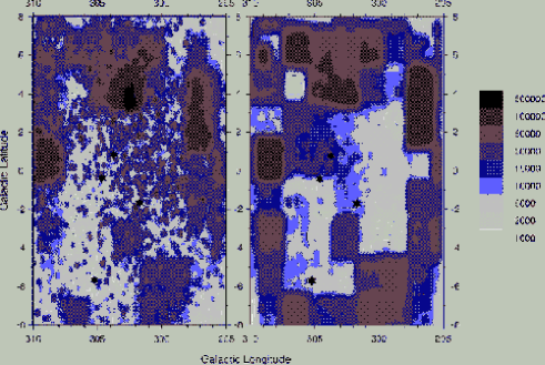
Figure 4: The emission predicted by our model with different values of $\it{a}$ and $\it{g}$ are shown here - $\it{a}$ = 0.3; $\it{g}$ = 0.9 on the left and $\it{a}$ = 0.5; $\it{g}$ = 0.1 on the right and the scale is shown on the right. The locations of the 5 $\it{Voyager}$ observations are shown in the images as stars - note that one of the locations was observed with both $\it{Voyager}1$ and $\it{Voyager}2$.

By comparing our model runs with the observations (Table 3), we have found that the best fit value for the albedo is $\it{a}$ = 0.4 $\pm$ 0.1 with 90% confidence contours as shown in Fig. 3. Unfortunately, we cannot similarly constrain $g$. The primary reason for this is seen in Fig. 4 where we have plotted the distribution of the scattered starlight for both isotropic and forward scattering grains. Because the locations of the 5 $\it{Voyager}$ targets (shown as large stars in Fig. 4) were essentially chosen at random, the observations at those positions can be matched by any value of $g$.

There are very few determinations of the optical constants of interstellar grains in the FUV and none have been of grains in the diffuse ISM (see Draine 2003a; Gordon 2004). The albedo derived here is consistent with that from observations of reflection nebulae (Witt et al. 1993; Calzetti et al. 1994; Burgh et al. 2002). Although our observations cannot distinguish between different values of $g$, we have proposed new observations in regions selected such that we can unambiguously determine the optical constants.

Table 2: Table of column density measurements for various stars in the region. References: 1. SIMBAD; 2. Franco (1989); 3. Seidensticker (1989); 4.Franco (2000); 5. York & Rogerson (1976); 6. Shull & Steenberg (1985); 7. Bohlin et al. (1983); 8. Crawford (1991)

HD Number	Dist	N(H)	$\it{l}$	$\it{b}$	Ref.
	(pc)	($\times 10^{20}$$cm^{-2}$)	(deg)	(deg)
58806	294.9	20.8	296.764	3.55	1
94493	980.4	13.3	289.0	-1.20	1
97617	284.1	8.7	293.5	-6.04	1
98195	284.1	5.8	294.9	-8.53	1
99149	157.7	5.2	294.1	-4.47	1
99857	483.1	23.7	294.8	-4.90	1
100101	284.9	45.2	294.5	-3.48	1
100666	178.3	11.6	294.6	-2.33	1
100990	255.1	11.0	296.4	-7.33	1
100927	238.7	42.3	293.5	2.06	1
101190	237.1	24.3	294.8	-1.50	1
101903	249.3	41.7	295.9	-3.44	1
101929	145.6	9.3	293.3	6.40	1
101190	237.1	10.9	294.8	-1.49	1
101966	135.8	5.2	296.8	-6.42	1
102461	251.8	30.9	294.4	4.11	1
102544	255.1	7.5	297.0	-5.63	1
102349	709.0	30.1	295.0	1.63	1
102728	190.6	53.3	295.4	1.52	1
102386	189.4	30.7	295.5	-0.36	1
103066	303.0	12.7	296.6	-2.46	1
103168	362.0	44.0	296.2	-0.35	1
103079	103.7	0.2	296.7	-3.05	8
103101	104.5	1.0	294.9	4.95	1
104432	628.0	6.4	297.2	-0.29	1
104841	230.9	8.5	297.6	-0.77	1
104936	251.8	34.2	298.9	-7.49	1
104479	216.4	26.1	298.5	-6.75	1
104125	96.7	5.8	295.9	4.99	1
104564	253.8	2.3	296.2	5.67	1
105017	395.0	33.0	298.1	-2.44	1
105194	254.5	4.0	297.6	1.21	1
105822	288.2	33.0	299.2	-5.68	1
105907	460.8	27.8	297.5	5.65	1
106521	411.0	11.6	298.6	1.53	1
106490	111.6	1.1	298.2	3.79	7
107652	313.5	4.9	299.6	0.47	1

Hipparcos number.

Table 2: continued

HD Number	Dist	N(H)	$\it{l}$	$\it{b}$	Ref.
	(pc)	($\times 10^{20}$$cm^{-2}$)	(deg)	(deg)
107821	97.9	5.8	299.9	-1.16	1
107411	146.0	7.5	302.1	-1.34	4
107978	295.9	6.6	299.7	1.82	1
107082	184.5	34.2	298.9	2.41	1
107983	191.2	10.4	300.7	-7.96	1
107789	151.1	2.3	299.1	5.88	1
108395	268.1	34.8	299.8	4.40	1
108750	133.9	1.2	300.4	1.31	1
108804	217.4	1.2	300.5	0.95	1
108813	68.2	1.7	300.5	1.37	1
108531	343.6	8.1	300.2	0.68	1
108610	378.8	8.4	300.3	0.88	1
108939	2272.7	6.9	300.5	1.89	1
108447	166.6	26.1	301.0	-7.76	1
108248	98.3	0.4	300.1	-0.36	5
108355	201.6	8.4	300.3	-1.04	4
108483	135.8	3.6	299.1	12.50	1
108671	186.5	2.9	300.8	-3.82	1
108608	1068.3	5.5	300.2	1.82	1
108999	636.6	6.6	300.6	0.96	1
109000	73.7	0.3	300.8	-0.72	1
109266	589.8	5.8	300.9	1.03	1
109493	660.8	8.9	301.1	-0.06	1
109504	676.1	11.0	301.1	1.31	1
109810	1015.8	9.8	301.4	1.03	1
109152	110.3	8.1	301.3	-6.02	1
109475	83.6	3.8	301.1	1.07	1
109550	403.2	7.5	301.2	-0.02	1
109801	105.5	3.7	301.6	-2.99	3
109165	156.3	8.1	301.3	-6.02	1
109047	239.2	13.3	300.7	0.29	1
109199	387.6	14.2	301.1	-3.31	1
109478	125.3	4.1	301.3	-2.46	1
109563	188.3	2.4	301.5	-4.34	1
109614	313.5	4.1	301.5	-4.38	1
109891	151.3	13.3	301.5	0.31	1
109993	277.0	11.6	301.8	-4.19	1
109777	121.4	6.9	301.1	4.95	1
109993	277.0	10.4	301.8	-4.19	1
113153	120.9	1.2	304.0	-5.19	1
114911	124.4	0.6	305.2	-5.12	1

Table 2: continued

HD Number	Dist	N(H)	$\it{l}$	$\it{b}$	Ref.
	(pc)	($\times 10^{20}$$cm^{-2}$)	(deg)	(deg)
115267	231.5	11.6	305.5	-4.21	1
112254	255.1	4.6	303.4	-4.75	1
112938	189.3	8.1	303.9	-5.0	1
115583	169.5	2.8	305.7	-4.64	1
113558	178.9	2.9	304.3	-5.73	1
116424	172.7	20.2	306.1	-5.86	1
115286	225.2	6.3	305.4	-5.74	1
113590	141.8	1.2	304.3	-5.32	1
114142	144.3	0.6	304.7	-4.74	1
113607	540.5	1.7	304.3	-4.91	1
116230	163.4	0.6	306.1	-4.18	1
112764	73.9	9.3	304.1	6.94	1
115842	102.1	30.7	307.1	6.83	1
115436	278.5	8.9	306.6	5.38	1
111302	190.5	11.6	302.6	4.42	1
113455	184.2	15.0	304.7	4.24	1
114808	165.5	26.6	305.9	4.42	1
117171	188.6	34.2	308.1	4.92	1
110390	105.1	8.1	301.8	1.83	1
110772	223.7	30.1	302.1	2.78	1
113199	139.2	8.7	304.4	2.84	1
112556	193.7	18.6	303.8	4.38	1
116087	108.7	0.4	306.7	1.65	8
116780	202.4	9.3	307.4	2.85	1
119385	220.3	12.7	309.6	2.30	1
113919	306.7	3.5	304.6	-4.97	1
116749	138.3	1.0	306.5	-4.12	1
116849	480.0	20.8	306.6	-3.67	1
117651	106.9	1.0	307.3	-3.11	1
117652	221.7	29.5	307.1	-4.20	1
113956	287.0	8.1	304.5	-6.90	1
115286	225.2	6.3	305.4	-5.74	1
116865	152.9	11.0	306.4	-5.24	1
117445	125.6	8.7	306.6	-6.65	1
116106	178.9	10.4	305.8	-6.10	1
118229	261.1	12.1	307.1	-6.47	1
110511	192.7	8.1	302.3	-8.17	1
111442	253.1	9.3	302.9	-8.75	1
114887	289.8	12.6	304.9	-7.69	1
118684	293.2	10.4	307.2	-7.52	1

Table 2: continued

HD Number	Dist	N(H)	$\it{l}$	$\it{b}$	Ref.
	(pc)	($\times 10^{20}$$cm^{-2}$)	(deg)	(deg)
118344	134.4	26.7	306.9	-7.93	1
118522	308.6	27.1	306.9	-8.29	1
118846	205.1	38.4	308.6	-0.17	1
119661	510.0	12.1	308.8	-2.43	1
111037	117.7	0.9	302.4	1.64	2
112123	179.2	5.6	303.4	0.30	3
110640	194.1	16.0	302.1	1.33	3
111580	111.0	4.0	302.9	-2.04	3
110151	751.9	11.3	301.6	1.93	1
110020	108.3	3.6	301.8	-3.67	1
111283	1250.0	11.7	302.7	-2.72	1
112607	304.9	15.6	303.8	-0.78	1
112766	303.0	4.4	303.8	-3.99	1
113991	671.1	20.5	305.0	1.87	1
114603	680.3	10.7	305.5	1.30	1
110310	135.7	4.9	302.0	-1.88	1
110477	78.8	17.4	301.9	1.71	1
110610	146.2	5.8	302.1	-1.35	1
111161	97.7	5.2	302.6	-4.26	1
111303	354.6	9.2	302.7	1.80	1
112109	96.3	0.6	303.3	-0.77	1
112703	63.0	9.3	303.8	-1.51	1
110062	507.6	17.6	301.7	-0.61	1
110079	271.0	11.3	301.8	-3.01	1
110163	467.3	15.3	301.7	0.86	1
110245	671.1	6.4	302.0	-4.12	1
110715	352.1	21.1	302.2	-2.10	1
110737	174.5	24.0	302.3	-2.46	1
110830	163.4	12.7	302.3	0.67	1
110925	221.2	10.4	302.3	2.03	1
110946	925.9	26.3	302.4	-2.05	1
111409	383.1	15.3	302.8	-1.74	1
111992	518.1	27.8	303.2	-0.30	1
112169	145.9	2.3	303.4	-0.26	1
112295	320.5	38.0	303.6	1.53	1
112954	613.5	28.7	304.1	-0.08	1
113191	265.3	8.7	304.2	-1.94	1
113457	95.1	1.5	304.4	-1.61	1
113689	232.5	6.4	304.6	-1.74	1
114792	2777.0	29.0	305.5	0.10	1

Table 2: continued

HD Number	Dist	N(H)	$\it{l}$	$\it{b}$	Ref.
	(pc)	($\times 10^{20}$$cm^{-2}$)	(deg)	(deg)
114012	540.5	26.6	304.9	-0.40	1
114670	2702.7	5.8	305.4	-0.53	1
114738	211.4	8.7	305.4	-1.55	1
114739	236.4	4.8	305.3	-2.27	1
111557	205.5	3.5	302.9	-0.12	1
112045	196.0	30.8	303.3	1.07	1
112225	139.8	1.7	303.5	1.95	1
113348	337.2	9.8	304.4	1.37	1
110373	1447.0	16.2	301.9	-0.12	1
110956	121.4	3.6	302.2	6.40	1
112026	2476.7	15.9	303.3	1.98	1
112536	492.8	17.1	303.8	1.84	1
110433	879.0	24.9	302.0	-0.33	1
110449	1488.5	19.1	301.9	1.88	1
110736	771.6	20.3	302.2	-0.11	1
110975	616.9	22.0	302.4	-0.28	1
111024	566.7	22.0	302.4	-0.22	1
111687	618.2	5.2	303.0	1.79	1
111827	473.4	16.8	303.1	-1.95	1
112637	978.2	30.7	303.8	-0.45	1
113014	1612.5	30.1	304.1	0.67	1
113511	2721.2	42.9	304.5	-1.22	1
113658	707.4	11.3	304.7	1.68	1
113968	1094.9	13.9	305.0	1.56	1
114317	1105.6	7.8	305.3	1.82	1
114318	681.2	10.7	305.3	1.40	1
114460	541.4	5.8	305.3	0.48	1
112485	2286.7	16.2	303.7	2.05	1
112078	110.4	10.0	303.4	3.7	6
118716	115.2	5.7	310.2	8.70	1
120359	262.4	5.8	310.6	3.48	1
120768	83.6	4.6	310.6	1.93	1
120891	235.8	7.5	309.1	-4.78	1
121796	195.3	4.1	310.0	-3.60	1
122036	315.4	4.6	309.2	-7.03	1
122098	361.0	4.8	310.5	-2.39	1
122144	161.0	0.4	310.9	-1.17	6
122451	161.0	2.6	311.8	1.25	1
124316	353.3	5.8	310.6	-6.92	1