The Deuterium-to-Hydrogen Ratio in a Low-Metallicity Cloud Falling onto the Milky Way

Abstract

Using Far Ultraviolet Spectroscopic Explorer (FUSE) and Hubble Space Telescope (HST) observations of the QSO PG 1259+593, we detect D I Lyman-series absorption in high velocity cloud Complex C, a low-metallicity gas cloud falling onto the Milky Way. This is the first detection of atomic deuterium in the local universe in a location other than the nearby regions of the Galactic disk. We construct a velocity model for the sight line based on the numerous O I absorption lines detected in the ultraviolet spectra. We identify 8 absorption-line components, two of which are associated with the high velocity gas in Complex C at $\approx-128$ and $\approx-112$  km s^-1. A new Westerbork Synthesis Radio Telescope (WSRT) interferometer map of the H I 21 cm emission toward PG 1259+593 indicates that the sight line passes through a compact concentration of neutral gas in Complex C. We use the WSRT data together with single-dish data from the Effelsberg 100-meter radio telescope to estimate the H I column density of the high velocity gas and to constrain the velocity extents of the H I Lyman-series absorption components observed by FUSE. We find N(H I) = $(9.0\pm 1.0)\times 10^{19}$ cm^-2, N(D I) = $(2.0\pm 0.6)\times 10^{15}$ cm^-2, and N(O I) = $(7.2\pm 2.1)\times 10^{15}$ cm^-2 for the Complex C gas (68% confidence intervals). The corresponding light-element abundance ratios are D/H = $(2.2\pm 0.7)\times 10^{-5}$, O/H = $(8.0\pm 2.5)\times 10^{-5}$, and D/O = $0.28\pm 0.12$. The metallicity of Complex C gas toward PG 1259+593 is approximately 1/6 solar, as inferred from the oxygen abundance [O/H] = $-0.79\pm^{0.12}_{0.16}$. While we cannot rule out a value of D/H similar to that found for the local ISM (i.e., D/H $\sim 1.5\times 10^{-5}$), we can confidently exclude values as low as those determined recently for extended sight lines in the Galactic disk (D/H $<1\times 10^{-5}$). Combined with the sub-solar metallicity estimate and the low nitrogen abundance, this conclusion lends support to the hypothesis that Complex C is located outside the Milky Way, rather than inside in material recirculated between the Galactic disk and halo. The value of D/H for Complex C is consistent with the primordial abundance of deuterium inferred from recent Wilkinson Microwave Anisotropy Probe (WMAP) observations of the cosmic microwave background and simple chemical evolution models that predict the amount of deuterium astration as a function of metallicity.

1 Introduction

Observations of the abundance of deuterium relative to hydrogen (D/H) in different environments provide insight into the evolution of the light elements in the universe. With the excellent concordance in the estimates of the cosmic baryon density from measurements of D/H in low-metallicity quasar absorption-line systems and measurements of the cosmic microwave background, the cosmic baryon density and the primordial value of D/H are now tightly constrained (Burles, Nolett, & Turner 2001; O’Meara et al. 2001; Spergel et al. 2003). Thus, it should be possible to test chemical evolution models by examining the progression of D/H with time (see Lemoine et al. 1999 and Olive, Steigman, & Walker 2000 for recent discussions). The abundance of deuterium is expected to decrease with time since there are no known sources of deuterium capable of increasing the cosmic abundance significantly (Epstein, Lattimer, & Schramm 1976; see also Prodanović & Fields 2003). Many chemical evolution models predict moderate levels of deuterium destruction by stellar nucleosynthesis, typically less than a factor of 3–5 (Clayton 1985; Edmunds 1994; Steigman & Tosi 1995; Tosi et al. 1998). More recent models suggest that slightly lower levels of astration are also possible (e.g., Chiappini, Renda, & Matteucci 2002).

Unfortunately, measurements of D/H are particularly difficult, and there have been relatively few opportunities to directly measure the detailed changes in the abundance of deuterium as a function of metallicity or time. A key piece of information missing in discussions of the evolution of the light element abundances with time is the behavior of D/H in environments with metallicities between those of the high-redshift systems (typically $Z\lesssim 0.01Z_{\odot}$) and those of gas in the local neighborhood of the Sun (typically $Z\sim Z_{\odot}$).

There are several reasons why it it is important to determine the D/H ratio in a wide variety of galactic and extragalactic environments. First, there have been few high-precision estimates of D/H at moderate to high redshifts ($z\sim 2-4$), where the amount of stellar processing of deuterium is presumably low, as evidenced by low metallicity (e.g., O’Meara et al. 2001; Pettini & Bowen 2001 and references therein). The measurements that have been made appear to yield conflicting values for the primordial abundance of deuterium, with the observed values depending on the type of system observed (e.g., Lyman-limit or damped Ly$\alpha$ systems – see Pettini & Bowen 2001). Second, estimates of D/H in many locations yield a more global perspective of the chemical history of gas at different epochs than is possible from a few isolated measurements. Chemical evolution models seeking to describe the general evolution of the light-element abundances need a large sample of measurements to avoid systematic problems encountered by relying upon data for only a few types of environments. Third, although measurements of deuterium in nearby gas clouds imply a relatively constant value of D/H within the local interstellar medium (ISM; Moos et al. 2002 and references therein), substantial variations may exist in D/H and D/O over distances of only a few hundred parsecs (Jenkins et al. 1999; Sonneborn et al. 2000; Hoopes et al. 2003; Hébrard & Moos 2003). If a sufficiently large number of high-precision D/H and D/O measurements can be made in a diverse set of nearby environments, it may be possible to understand the exact causes of this variability and the degree to which galactic chemical evolution and accretion of intragroup gas clouds influence the scatter in the observed ratios, both locally and at high redshift. This goal is a major science driver for the Far Ultraviolet Spectroscopic Explorer (FUSE) mission (Moos et al. 2000).

To bridge the gap in D/H between low and high metallicity environments, we have obtained an extensive set of FUSE, Hubble Space Telescope (HST), and interferometric H I 21 cm observations of the quasar PG 1259+593 behind high velocity cloud (HVC) Complex C. The HVC is located at least 3.5 kpc from the Galactic plane (Wakker 2001), well beyond all Milky Way clouds with current D/H determinations. Unlike previous investigations of D/H and D/O in either high-redshift clouds or the local ISM, we know which gaseous system is responsible for the high-velocity D I Lyman-series absorption observed toward PG 1259+593. A global description of the gas in Complex C is available from both emission and absorption-line measurements. The neutral gas in Complex C has been mapped extensively in H I 21 cm emission (see Wakker 2001 and references therein) and low-ionization absorption (e.g., Wakker et al. 1999; Richter et al. 2001b; Collins, Shull, & Giroux 2003). The ionized gas in Complex C has been investigated in absorption by Sembach et al. (2003) and Fox et al. (2003), and in emission by Tufte, Reynolds, & Haffner (1998) and Wakker et al. (1999). Complex C is an excellent site to determine D/H for comparisons with the high-redshift values because it is chemically young (Richter et al. 2001b; Collins et al. 2003; Tripp et al. 2003) and has a metallicity (10–25% solar) lower than that of the general ISM of the Milky Way and higher than that of intergalactic clouds at high redshifts.

In this paper we describe these new measurements and the resulting D/H and D/O ratios in Complex C. In §2 we describe the FUSE and HST Space Telescope Imaging Spectrograph (HST/STIS) absorption-line observations and the H I 21 cm interferometer observations. Section 3 contains a short summary of the properties of the PG 1259+593 sight line. In §4 we outline the methods and general assumptions used to determine the column densities of H I, D I, and O I in Complex C. We determine the H I column density from interferometric H I 21 cm emission data and use the FUSE and HST/STIS ultraviolet absorption-line data to determine the O I and D I column densities. Sections 5, 6, and 7 contain descriptions of these determinations for oxygen, hydrogen, and deuterium, respectively, and provide estimates of the various errors. The column densities and error ranges are summarized and discussed in §8, and comments on future progress appear in §9. We summarize the results of the study in §10.

2 Observations

2.1 Far Ultraviolet Spectroscopic Explorer Observations

We observed PG 1259+593 on nine occasions with FUSE between 2000 February 25 and 2001 March 28 for a total (orbital day + night) integration time of $\sim 600$ kiloseconds (ks) spread over 236 individual exposures. Approximately 350 ks of data were obtained during orbital night. An observation log for the nine visits is provided in Table 1. Data were obtained through the large (LWRS; $30\arcsec\times 30\arcsec$) apertures in all four FUSE channels (LiF1, LiF2, SiC1, SiC2) with varying degrees of success. PG 1259+593 was always well-centered in the LWRS aperture of the LiF1 channel used for guiding, but thermal effects caused the light of PG 1259+593 to drift around inside (and at times even partially outside) the remaining three apertures. Detector high voltages were also at reduced levels during some of the exposures as a result of operational difficulties (see Table 1 notes). We obtained all of the data in time-tagged photon-address mode to allow for data screening and time-dependent corrections necessary to fully calibrate the data. The raw FUSE data for PG 1259+593 can be found in the Multi-Mission Archive at the Space Telescope Science Institute under the observation identifications P1080101–P1080109.

We processed the data with a customized version of the FUSE pipeline software (CALFUSE v2.2.2), which is publicly available from the FUSE Project at the Johns Hopkins University. The details of this processing follow the same general principles outlined by Sembach et al. (2001b). However, since PG 1259+593 is a faint object ($F_{\lambda}\sim 2\times 10^{-14}$ erg cm^-2 s^-1 Å^-1 between 920 and 1200 Å), we modified these procedures in the following manner to process the data. First, we screened the raw photon lists in every exposure for Earth limb avoidance, South Atlantic Anomaly passage, pulse height distribution constraints, and particle event bursts (see Sahnow et al. 2000). We chose the pulse height restrictions after inspection of the pulse height profiles to reduce background events while minimizing the number of source events discarded; pulse height data numbers from 4 to 24 were allowed. Event bursts were common in these observations, particularly those obtained in the March 2001 time period, so we carefully checked the cleaned lists to be sure that no obvious signal from these events remained after screening.

Next, we combined the screened exposure lists for each channel within each observation using the default spectral registration provided by the software. This default assumption is necessary since there is not enough signal in the individual exposures to reliably cross-correlate the positions of narrow spectral features; the typical exposure time of $\sim 2-3$ ks per exposure yielded an average of $\sim 2-3$ counts per resolution element in the highest sensitivity (LiF1) channel and $\sim 1-2$ counts per resolution element in the SiC channels. The summed channel lists for each observation were corrected for geometric distortions, Doppler shifts, thermally-induced grating motions, astigmatism, detector backgrounds, and scattered light following the standard procedures (Sahnow et al. 2000). The extracted spectra for each channel in each observation were then flux calibrated and wavelength calibrated. We registered the spectra from each of the nine observations to a common wavelength scale by noting the integral pixel shifts required to align the same narrow absorption features observed in each spectrum. These shifts were typically less than 3 detector FUSE pixels and always less than 15 pixels. We then co-added the aligned spectra for all 9 observations to produce a final composite spectrum for each channel.

We registered the composite channel spectra to a common heliocentric wavelength scale by performing a channel-to-channel registration similar to that performed at the observation level and then setting the zero point of the wavelength scale to that provided by the STIS spectra (discussed below). For the FUSE-to-STIS registration, we compared the velocities of lines of the same species observed by each instrument (e.g., C II $\lambda\lambda 1036.337,1334.532$; Si II $\lambda\lambda 1020.699,1304.370$; Fe II $\lambda\lambda 1144.938,1608.451$). The C II and Fe II comparisons used lines with approximately the same line strengths, $f\lambda$, to ensure that the comparisons were not influenced by asymmetric profiles that saturate in one line but not the other. Additional checks were performed using cross-element comparisons (e.g., Si II $\lambda 1020.699$ with S II $\lambda\lambda 1250.584,1253.811$, etc.). We then corrected the FUSE spectra to the Local Standard of Rest (LSR) reference frame. For the PG 1259+593 sight line, the correction for standard solar motion $v_{\rm LSR}=v_{\rm helio}+10.5$  km s^-1, assuming a solar speed of 19.5  km s^-1 in the direction $l_{std}=56\arcdeg$, $b_{std}=23\arcdeg$ (Delhaye 1965; Lang 1980; see also Kerr & Lynden-Bell 1986). This correction is within $\approx 1.6$  km s^-1 of the LSR reduction based on a solar speed of 16.5  km s^-1 in the direction $l=53\arcdeg,b=25\arcdeg$ (Mihalas & Binney 1981). Unless stated otherwise, all velocities quoted in this paper are in the LSR reference frame. The FUSE spectra for PG 1259+593 have a nominal zero-point velocity uncertainty of $\pm 5$  km s^-1 ($1\sigma$) after these calibrations have been applied.

The FUSE data are oversampled in the spectral domain. Therefore, after calibration we binned the spectra to a spectral bin size of 4 pixels, or $\sim 0.025$ Å ($\sim 7.5$  km s^-1). This binning provides approximately 3 samples per spectral resolution element of 22–25  km s^-1. The night-only data used in this study have continuum signal-to-noise ratios $S/N\sim 25$ and 16 per spectral resolution element at 1030 Å in the LiF1 and LiF2 channels, respectively, and $S/N\sim 10$ and 12 at 950 Å in the SiC1 and SiC2 channels, respectively.

The version of CALFUSE (v2.2.2) used for this study has significant improvements over earlier versions used in previous studies, most notably improved wavelength solutions and background corrections tailored for day+night or night-only extractions. Portions of the fully reduced night-only SiC2 and SiC1 spectra in the 915–955 Å wavelength range are shown in Figure 1. The locations of the Lyman series H I and D I lines are indicated in the top panel along with the locations of prominent interstellar O I and N I lines. Terrestrial airglow emission features, which are present in all of the H I lines observed, are marked below the top spectrum with crossed circle symbols. Terrestrial O I and N I emissions are undetectable in the night-only data shown. The background subtraction for both channels results in nearly zero residual flux in the cores of the H I lines as expected, except at velocities affected by airglow contamination. (A similar conclusion holds for the very strong C II $\lambda 1036.337$ line observed in all four channels.) The slight rise in the sub-Lyman-limit regime ($\lambda<912$ Å) in the SiC1 channel may be the result of the radiative recombination continuum emission from atomic oxygen near 911 Å (see Feldman et al. 1992; López-Moreno et al. 2001) or improper background subtraction at these very short wavelengths. The SiC2 channel extends only to 916.6 Å, so no independent check of the SiC1 behavior at $\lambda<916$ Å is possible.

In the discussions that follow, we restrict our analysis to the orbital night-only data to minimize the impact of terrestrial H I and O I airglow emissions on the absorption lines of interest in this study. In particular, we concentrate on data from the two SiC channels covering the FUSE bandpass below 1000 Å, but we also use the independent data from the two LiF channels to check the quality of the data at longer wavelengths. The checks allowed by multiple channel observations of the same spectral region are important for assessing noise in the data. When we derive H, D, and O abundances, we use both the SiC1 and SiC2 data. Additional illustrations of FUSE spectra of PG 1259+593 can be found in Richter et al. (2001b) and Wakker et al. (2003).

2.2 Space Telescope Imaging Spectrograph Observations

PG1259+593 was observed several times with HST/STIS as part of Guest Observer program GO-8695 on 2001 January 17-19 and 2001 December 19. An observation log is provided in Table 2. All observations used the intermediate-resolution echelle mode (E140M) and the $0\farcs 2\times 0\farcs 06$ slit to minimize the power in the wings of the spectral line-spread function (see Figure 13.90 in the STIS Instrument Handbook, Leitherer et al. 2002). This instrument mode provides a resolution of $\sim 7$  km s^-1 (FWHM) per two-pixel resolution element and covers the 1150–1729 Å wavelength band with only five small gaps between echelle orders at $\lambda>$ 1634 Å. For further details on the design and performance of STIS, see Woodgate et al. (1998) and Kimble et al. (1998).

We reduced the data for each observation in the manner described by Tripp et al. (2001), including application of the two-dimensional scattered light correction developed by the STIS Team (Landsman & Bowers 1997; Bowers et al. 1998). We weighted the extracted flux-calibrated spectra for each observation by their inverse variances and added them together to produce a composite spectrum. The continuum signal-to-noise ratio per resolution element in the final co-added spectrum ranges from $\sim$7 to 17 and peaks near 1400 Å. We corrected the STIS data to the LSR reference frame by adding +10.5  km s^-1 to the nominal heliocentric velocity scale provided by the standard processing. The zero-point accuracy of the STIS velocity scale for these data is approximately $\pm 1$  km s^-1.

Examples of continuum normalized profiles for the absorption lines of several low ionization species are shown in Figure 2. Additional examples of absorption lines in these STIS spectra of PG 1259+593 can be found in Richter et al. (2003) and Collins et al. (2003).

2.3 H I 21 cm Observations

High velocity clouds often show structure at angular scales down to at least $\sim$1′ (e.g., Wakker & Schwarz 1991), particularly in cloud cores. The PG 1259+593 sight line samples the Complex C core named CIII (Giovanelli, Verschuur, & Cram 1973; Wakker 2001). The Leiden-Dwingeloo Survey (LDS, Hartmann & Burton 1997) shows that this core has an extent of about $1\arcdeg\times 2\arcdeg$ at a column density of $3\times 10^{19}$ cm^-2, with PG 1259+593 lying at its edge. To determine a more accurate estimate of the amount of high velocity H I in this region of the sky, we observed CIII with the Westerbork Synthesis Radio Telescope (WSRT). Since this interferometer filters out the large-scale structure, we supplemented the WSRT data in the direction of PG 1259+593 with an Effelsberg single-dish observation having a 9$\farcm$7 beam. This latter observation is described by Wakker et al. (2001).

The half-power beam width (HPBW) of the WSRT primary beam is 35′, which allows an area with a diameter of about 44′ to be mapped. We therefore observed CIII with a mosaic of $2\times 4$ pointings spaced 27′ apart, resulting in mapping over an area of $(22\arcmin+27\arcmin+22\arcmin)\times(22\arcmin+3\times 27\arcmin+22\arcmin)=71\arcmin\times 125\arcmin$ arc minutes. To increase the sensitivity, we included an extra pointing in the direction of PG 1259+593 itself. For each of these pointings, we obtained full uv-plane coverage in $4\times 12$ hours, using shortest spacings of 36, 54, 72, and 90 m. The correlator was set to cover the LSR velocity range between $-333$ and +197  km s^-1 with 2.1  km s^-1 velocity resolution after on-line Hanning smoothing was applied. The WSRT observations were completed in late April 2001.

R. Braun of the Netherlands Foundation for Research in Astronomy performed the calibration of the observations. The calibrated data were mapped using uniform weighting, and included a Gaussian taper in the uv-plane such that the final synthesized beam is $1\arcmin\times 1\arcmin$. Next, a map of the continuum was created for each pointing by adding the channels without H I emission. After subtracting the continuum, the individual pointings were cleaned using the Multi-Resolution Clean algorithm (Wakker & Schwarz 1988). To increase the accuracy of this step, the areas containing signal were first delineated, taking into account the overlap between pointings. The resulting cleaned maps were then mosaiced together. The fully processed data have a final root-mean-square (RMS) residual of $\sim 3.2$ mJy beam^-1, or $\sim 0.5$ K.

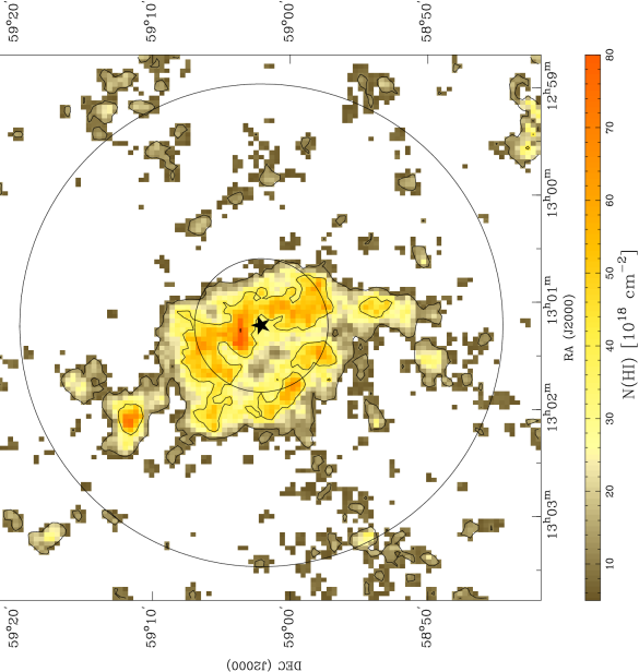
Figure 3: Filtered H I column density of the WSRT data, integrated over the velocity range $-148$ to $-109$  km s^-1, which includes core CIII. There is a slowly varying offset of $(3.0-6.0)\times 10^{19}$ cm^-2 across the field that is not included in this estimate because it has been filtered out by the interferometer. At the position of PG 1259+593, marked by the star at $\alpha$=13^h01^m13^s, $\delta$=59^∘02^′06^′′, this offset is $6\times 10^{19}$ cm^-2. The circles centered on PG 1259+593 show the FWHM of the Effelsberg and Westerbork primary beams.

Figure 3 shows a grey-scale map of N(H I) for Complex C core CIII based on the WSRT data (integrated between $-$148 and $-$109  km s^-1). PG 1259+593 lies in the brightest concentration in the field, which coincides with the brightest spot in the LDS data. Although it seems unusual that the extragalactic background source lies toward the center of a cloud core, this is not an artifact of the mosaic process; if the pointing centered on PG 1259+593 is removed, the core is still clearly seen at the half-power point of each of the four surrounding pointings, and the final H I map looks similar, though noisier. We discuss the H I data and the derived column density for the high velocity gas in §6.1.

3 The PG 1259+593 Sight Line

PG 1259+593 lies in the direction $l=121\fdg 09,~{}b=+57\fdg 80$ behind HVC Complex C, which spans Galactic longitudes between $l\sim 30\arcdeg$ and $l\sim 150\arcdeg$ in the northern Galactic hemisphere. Maps of the H I 21 cm emission in Complex C can be found in Wakker (2001) and Sembach et al. (2003); these maps show larger regions than the area around the sight line covered in Figure 3. Complex C has a mass M $>1.2\times 10^{6}$ M_⊙ and a distance $d>5$ kpc (or altitude z $>$ 3.5 kpc) (van Woerden et al. 1999). Wakker (2001) suggests a distance limit $d>6.1$ kpc and a mass M $>3\times 10^{6}$ M_⊙. Various determinations of the metallicity of the high velocity gas yield $Z/Z_{\odot}\sim 0.1-0.3$ on a linear scale where $Z=Z_{\odot}$ is solar (Wakker et al. 1999; Gibson et al. 2001; Collins et al. 2003; Tripp et al. 2003). Previously, Richter et al. (2001b) found $Z/Z_{\odot}=0.093\pm^{0.125}_{0.047}$ for Complex C based on a subset of the oxygen absorption lines toward PG 1259+593 considered here.

In the direction of PG 1259+593, interstellar gas within 10 kpc of the Galactic plane that is participating in differential Galactic rotation has velocities $v_{LSR}\approx-30$ to 0  km s^-1. There is also a large intermediate-velocity cloud known as the Intermediate-Velocity Arch in this general direction (Kuntz & Danly 1996). Complex C has a velocity $v_{LSR}\approx-157$ to $-100$  km s^-1, which makes it possible to distinguish between the absorption produced by the HVC and the lower velocity foreground absorption produced by the nearby ISM ($v_{LSR}\sim-5$  km s^-1) and the Intermediate Velocity Arch (IV Arch; $v_{LSR}\sim-55$  km s^-1). The three principal groups of gas along the sight line are reasonably well separated in velocity in the H I 21 cm emission and weak ultraviolet absorption-line profiles shown in Figure 2. In the strongest absorption lines shown (Si II $\lambda 1526.707$, O I $\lambda 1302.168$, C II $\lambda 1334.532$), the ISM and IV Arch components blend together. It is important to note that the 21 cm emission associated with Complex C is stronger than that from the IV Arch or the Milky Way ISM in this direction, a point we will return to in the derivation of the Complex C H I Lyman series velocity structure in §6. Other sight lines through Complex C usually exhibit much weaker HVC 21 cm emission and/or have a much more complicated velocity structure that hinders a clean separation of the Complex C gas from the ISM and intermediate velocity gas. For examples of the 21 cm emission toward other sight lines passing through Complex C, see Sembach et al. (2003) and Wakker et al. (2001). The “enhanced” 21 cm emission toward PG 1259+593 is undoubtedly due to the fact that the sight line is located directly behind the Complex C core CIII (see §2.3).

In addition to neutral gas, Complex C contains ionized gas that can be traced through its H$\alpha$ emission (Tufte et al. 1998; Wakker et al. 1999), O VI absorption (Murphy et al. 2000; Sembach et al. 2000, 2003), and C IV and Si IV absorption (Fox et al. 2003; see also §6 below). We must consider the impact of these ionized regions on our derivation of D/H in Complex C since they may contain trace amounts of H I detectable in the H I Lyman series lines (see §6).

4 General Methodology

4.1 Overview

Even though the PG 1259+593 sight line has many desirable attributes that facilitate a detection of deuterium in Complex C, the conversion of this detection into a reliable estimate for the deuterium abundance depends upon many factors. It is necessary to take a methodical approach to determining the D/H and D/O ratios in the high velocity gas. The sight line is more complicated than short sight lines through the local ISM used to determine the local value of D/H (e.g., Moos et al. 2002 and references therein; Hébrard & Moos 2003). It is also more complex than the high-redshift sight lines, which can be selected for simple intergalactic absorption velocity structure and typically contain one or two predominant absorption components (e.g., O’Meara et al. 2001). The velocity structure of the PG 1259+593 sight line does not allow for a precise measure of the H I column density in Complex C solely through analysis of the H I Lyman-series absorption due to blending of the high velocity H I absorption with the ISM and IV Arch components. However, it is possible to derive an accurate H I column density from 21 cm emission, provided that the angular resolution is sufficiently high to assure that small-scale structure within the radio beam is not biasing the result. It is also possible to draw upon the information in the O I absorption profiles for the sight line and to constrain the range of possible Lyman-series absorption parameters for both D I and H I.

Our adopted method for determining the D/H and D/O ratios in Complex C can be broken down into several key steps: 1) determination of an accurate O I column density for Complex C and a model for the velocity structure of the neutral gas along the PG 1259+593 sight line using the numerous O I absorption lines in the FUSE and STIS spectra, 2) application of the O I velocity model to the H I Lyman-series lines in the FUSE data to create an H I model that reproduces the observed H I absorption and 21 cm emission profiles, 3) determination of the H I column density in Complex C from the interferometric H I 21 cm data described in §2.3, 4) determination of the amount of D I required to account for the Complex C absorption in the negative velocity wings of the H I Lyman-series lines, and 5) consideration of the uncertainties associated with steps (1) – (4).

4.2 Methods

We use a variety of spectral line analysis techniques to determine the velocity structure and column density of each species studied. Our primary tool for quantifying the properties of the absorption lines in the FUSE and HST/STIS spectra is a suite of software for fitting line profiles, written specifically for this study in the Interactive Data Language (IDL). The software constructs synthetic line profiles that can be compared to the observed data after convolution with an instrumental line spread function. It allows complex absorption lines to be modeled as a superposition of components with Maxwellian velocity distributions, each of which can be described as Voigt functions with appropriate natural damping constants. Each component has a central velocity ($\langle v_{i}\rangle$), line width (b_i), and column density (N_i), with the best-fit parameters found through a $\chi^{2}$-minimization of the differences between the model profiles and the data. To explore the sensitivity of our adopted results to various input parameters/assumptions and boundary conditions, we perform some of these profile fitting analyses multiple times with other profile fitting codes used in FUSE analyses of other sight lines (e.g., the Owens.f code – see Hébrard et al 2002; Lemoine et al. 2002). In all cases checked, the column densities are consistent to within the $1\sigma$ errors, confirming that the formal uncertainties have been estimated properly. For the O I and D I lines we also use curve-of-growth analyses to estimate column densities and to check the reliability of the profile fitting results. We describe these different analyses in the following discussions of the absorption produced by each species (H I, D I, O I).

4.3 Input Data and Reference Abundances

The input atomic data parameters for this study are known with high enough accuracy that they do not present a significant source of systematic uncertainty in our final results. We adopt wavelengths, oscillator strengths ($f$-values), and radiation damping constants from the atomic data compilations of Morton (1991, 2003). For O I, the original sources of the $f$-values are Zeippen, Seaton, & Morton (1977), Biémont & Zeippen (1992), and Tachiev & Froese Fischer (2002). The source of $f$-values for H I and D I is Pal’chikov (1998). We use multiple transitions of H I, D I, and O I in our line analyses. Thus, typical uncertainties of $10-20$% in the $f$-values for individual lines are mitigated by considering several transitions simultaneously in the column density determinations. To identify molecular hydrogen lines and assess their possible contamination of the atomic absorption features, we use the H₂ line lists of Abgrall et al. (1993a,b).

Throughout this work, we adopt a solar reference abundance (O/H)${}_{\odot}=4.90\times 10^{-4}$ from Allende Prieto, Lambert, & Asplund (2001). This reference solar oxygen abundance is in good agreement with the value of $4.5\times 10^{-4}$ derived from analyses of the solar [O I], O I, and OH line shapes and asymmetries implied by new 3-D hydrodynamical model atmospheres (Asplund 2003). It is in better agreement with the nearby average ISM oxygen abundance of (O/H)${}_{\rm ISM}=3.4\times 10^{-4}$ (Meyer 2001; Meyer, Jura, & Cardelli 1998) than earlier determinations based on 1-D model atmospheres. It also agrees well with recent determinations of H II region oxygen abundances (see Pilyugin, Ferrini, & Shkvarun 2003 and references therein). We will adopt this solar reference abundance in our discussions of the metallicities of the various absorbers along the sight line. Using (O/H)${}_{\odot}=5.45\times 10^{-4}$ from Holweger (2001) or (O/H)${}_{\odot}=7.41\times 10^{-4}$ from Grevesse & Noels (1993) yields values of [O/H] that are a factor of 0.05 dex and 0.18 dex lower, respectively, than those adopted in this study.

4.4 Simplifying Assumptions

4.4.1 Number of Components in the Model

Throughout this work, we adopt the minimum number of velocity components required to produce acceptable fits to the observed absorption lines in the FUSE and HST/STIS observations. Our choice of component structure is guided in part by the high-resolution HST/STIS data available for several metal-line species (e.g., O I, Si II, S II, Fe II). In all, 8 components are required to fit the O I, H I, and D I profiles. The attributes of these components will be discussed for each species in §§5–7. A standard F-test indicates that adding additional components does not significantly improve the quality of the fit to the observed data, with the possible exception of an additional weak H I absorption feature discussed in §7.1. Adopting fewer components does not provide an acceptable fit to both the O I and H I absorption-line data. Some of the identified components, especially those at low velocities, are likely to consist of multiple sub-components that cannot be resolved at the resolution of the FUSE and HST/STIS data.

4.4.2 Velocity Structure Assumptions in the Model

We require the O I, H I, and D I lines to have a similar velocity structure, but we do not simultaneously fit these species with other metal-line species (e.g., N I, Si II, S II, Fe II) as has been done in some previous D/H analyses of other sight lines. To do so would impose additional constraints on the O I, H I, and D I lines that are not only unwarranted but also potentially misleading for this sight line. The absorption profiles of other species may be influenced significantly by the presence of ionized gas in the different components along the sight line. Unlike sight lines to nearby stars where the coupling of many species makes sense because the velocity structure of the ISM is simple and the neutral and ionized species have very similar velocity structure (e.g., Vidal-Madjar et al. 1998; Hébrard et al. 2002), the PG 1259+593 sight line contains a variety of absorbing regions with a range of physical properties. Linking the O I velocity structure directly to the profile shapes of species that trace both neutral and ionized gas could result in an inferred velocity extent of the neutral Complex C absorption that is sensitive to the profile shapes of singly ionized species in Complex C or in the IV Arch gas at nearby velocities. A secondary concern with tying the velocity structure of O I to ions such as Si II or Fe II is the inclusion of refractory elements into dust. Differential depletion of elements into dust grains or selective shock-disruption of grains can alter the relative gas-phase abundances of ISM clouds encountered along the sight line, which in turn can translate into different absorption-line velocity structures for different species. We use all of the information available to construct an initial guess at the velocity structure of the sight line, but take the conservative approach of coupling the velocity structure of only those species (i.e., H I, D I, O I) for which ionization and dust depletion effects are unlikely to differ significantly. Information for the singly ionized species can be found in recent studies by Richter et al. (2001b) and Collins et al. (2003).

4.4.3 The FUSE Line Spread Function

We assume that the FUSE line spread function (LSF) has a Gaussian shape and a constant width (FWHM) of 0.075 Å ($\approx 12$ FUSE detector pixels) throughout the FUSE bandpass. This width corresponds to a velocity width of FWHM $\approx 20-25$  km s^-1, depending upon wavelength. This is slightly broader than the nominal value of 20  km s^-1 often assumed in FUSE studies (see Sahnow et al. 2000). It is reasonable to expect the LSF for the combined PG 1259+593 data to be degraded slightly compared to the nominal LSF for single FUSE exposures because the number of individual exposures in the combined set of observations is large and registration of the individual exposures is certain to introduce some minor spectral degradation, particularly in the SiC channels. Given the velocity structure of the sight line, it is difficult to find narrow isolated lines to determine the LSF width directly. The narrowest lines for which this is possible in the FUSE spectrum of PG 1259+593 have observed (instrumentally convolved) widths of $\approx 0.08$ Å (LiF1A detector segment) and $\approx 0.10$ Å (SiC2A detector segment). The measured widths are broader than the adopted LSF width but are consistent with the expected line widths based on the velocity structure observable at higher resolution in the STIS data shown in Figure 2.

In previous investigations of D/H along kinematically simple sight lines, a multiple-component LSF has sometimes been used to fit the data. For example, Kruk et al. (2002) and Wood et al. (2002) used a two-component LSF with a narrow component (FWHM = 9 pixels) containing $\sim 70-75$% of the total LSF area and a broad component (FWHM $=17-24$ pixels) containing $\sim 25-30$% of the LSF area. When summed, the double-Gaussian functions studied have a roughly Gaussian shape with a width similar to that adopted in this study. The resulting column densities of D I and O I obtained with a double-component LSF have been similar to those obtained with single-component LSFs (Kruk et al. 2002; Wood et al. 2002). The reasons for this are straight-forward: the nearby absorption is simple, and the effects of a broad LSF component are most pronounced for strongly saturated lines requiring very accurate estimates of the optical depth at low residual flux levels. Toward PG 1259+593, the velocity structure is much more complex. Since we must consider the case where weak absorption is in close proximity to strong absorption, it is not so easy to dismiss the effects of a non-Gaussian LSF. For our PG 1259+593 FUSE dataset, which is the combination of many individual exposures, the central-limit theorem implies that the LSF of the combined data should also closely represent a single Gaussian function. After modeling the sight line and considering the impact of a more complex LSF, we find that the addition of a second LSF component with broad wings does not change our estimates of the H I, D I, and O I line strengths. Other systematic uncertainties dominate the potential uncertainties caused by the adoption of a single-component LSF rather than a two-component LSF of the type used in previous FUSE studies.

We performed a consistency check on our LSF estimation by comparing the shape of the Fe II $\lambda 1144.938$ line in the FUSE LiF2A spectrum with that of the Fe II $\lambda 1608.451$ line in the HST/STIS spectrum. The two lines have intrinsic strengths ($f\lambda$) within $\sim 20\%$ of each other, so direct comparisons of the velocity structure and component absorption depths could be made by relating the FUSE spectrum to various smoothed versions of the higher resolution STIS spectrum. We found that a good approximation to the FUSE Fe II profile was obtained by convolving the STIS spectrum with a Gaussian function having FWHM $=20\pm 4$  km s^-1. (At 1145 Å, our adopted instrumental width of 0.075 Å corresponds to FWHM = 19.6  km s^-1.) Smaller smoothing widths left structure in the smoothed STIS spectrum that was not obvious in the FUSE data, while larger smoothing widths underestimated the line depths and overestimated the line widths of the FUSE absorption. This comparison does not reveal the exact shape of the FUSE LSF, but it is sufficient to bracket the LSF width and demonstrate that the adopted Gaussian LSF width is well-constrained.

4.4.4 Estimation of the Quasar Continuum

Another simplifying assumption we make is that there are no undulations in the ultraviolet continuum of PG 1259+593 on scales of less than a few Ångstroms. This assumption is made in essentially all studies of quasar absorption line spectra. Compared to the spectra of normal and degenerate hot stars, power-law quasar continua are exceedingly smooth over small wavelength intervals; see, for example, the FUSE spectrum of the quasar 3C 273 (Sembach et al. 2001b). The PG 1259+593 spectrum contains no signatures of a stellar population contribution to the continuum light, which can be difficult to model for some AGNs, particularly Type II Seyferts. We model the PG 1259+593 continuum in the vicinity of the interstellar lines as a smoothly varying function of wavelength. The low-order Legendre polynomial fits adopted for the SiC channel data below 960 Å are shown in Figure 1. The quasar continuum is relatively flat (i.e., d$F_{\lambda}$/d$\lambda\approx 0$) over the large wavelength interval considered ($\sim 900-1100$ Å). Uncertainties associated with the placement of these continua are small compared to the other sources of uncertainty discussed below. Continuum placement is especially important for the weak lines of D I, for which we have estimated upper limits including this systematic uncertainty. We used the methods outlined by Sembach & Savage (1992) to determine the continuum levels and to extract the continuum placement uncertainties.

4.4.5 Possible Contamination from Absorption Lines of Other Species

There is little molecular hydrogen along the PG 1259+593 sight line, as evidenced by the paucity of H₂ R(0) and R(1) Lyman-band absorption features in the FUSE spectra. Richter et al. (2001a) estimate $\sum_{J=0}^{1}\log{\rm N_{J}(H_{2})}$ $<13.96$ ($3\sigma$) in Complex C. There may be a small amount of H₂ absorption present in the strongest lines of the $J=0-3$ rotational levels at the velocities of the Milky Way ISM ($v_{\rm LSR}\approx-5$  km s^-1); we estimate $\sum_{J=0}^{3}\log{\rm N_{J}(H_{2})}$ $\approx 14.7$. A small amount of H₂ may also be present in the IV Arch [ $\sum_{J=0}^{3}\log{\rm N_{J}(H_{2})}$ = $14.0\pm^{0.21}_{0.44}$ ]. We examined each O I and D I line used in this study for possible interstellar H₂ lines that might be confused with the atomic absorption in Complex C at $-160\leq v_{LSR}\leq-110$  km s^-1. We found that the predicted interstellar H₂ lines in the $J=0-3$ rotational levels with the total column densities quoted above produce negligible absorption in the vicinity of these lines. H₂ absorption by the foreground ISM can safely be ignored in our analysis of the Complex C absorption features. Some H₂ lines arising in the Milky Way ISM occur at wavelengths corresponding to the low-velocity portions of the H I lines, but these features do not affect the inferred strengths or shapes of the strongly saturated H I lines.

There are no known absorption lines produced by the intergalactic medium (IGM) along the PG 1259+593 sight line at the wavelengths of the O I and D I lines between 915 Å and 950 Å. The strongest IGM systems occur at redshifts $z=0.04606$ and 0.21949 (Richter et al. 2003). In both cases the H I Lyman-series lines in these systems occur at wavelengths longward of the $910-950$ Å spectral region. The remaining 19 IGM systems with $z=0.00229-0.43148$ have H I detectable only in the Ly$\alpha$ $-$ Ly$\gamma$ transitions (Richter et al. 2003), so there is no possibility of contamination at shorter wavelengths by those systems. Of the possible metal-line species that are likely to be detectable, C III $\lambda 977.020$ tends to be the strongest and most common; it too is safely longward of the absorption features considered in this study. Potential redshifted extreme ultraviolet species (e.g., O II $\lambda 834.466$, O III $\lambda 832.927$, O IV $\lambda 787.711$) in the intergalactic absorbers along the sight line do not pose a problem either.

5 Oxygen

5.1 O I Velocity Structure

The first step in our study of the D/H ratio in Complex C is a determination of the O I velocity structure of the gas along the entire sight line in the velocity range $|v_{LSR}|\leq 300$  km s^-1. We use both the moderate-resolution FUSE observations of numerous O I lines at far-ultraviolet wavelengths, combined with the higher resolution HST/STIS echelle observations of the O I $\lambda 1302.168$ line, to examine the optical depth of the absorption in detail. (Note that the weak intersystem O I line at 1355.598 Å is not detected in the STIS spectrum.) Deriving the O I velocity structure is critical because it provides an excellent initial approximation to the velocity structure of the D I and H I lines and is required for an accurate metallicity ([O/H]) estimate for the Complex C gas.

The ionization fraction of O I is coupled to that of H I (and thus D I) through a strong charge exchange reaction at typical interstellar densities (Field & Steigman 1971):

$${\rm O^{+}(^{4}S_{3/2})+H^{0}\longrightarrow O^{0}(^{3}P_{2})+H^{+}+0.02~{}eV}.$$ (1)

Detailed CLOUDY photoionization models for a range of physical conditions spanning those likely to be encountered along the PG 1259+593 sight line show that the ionization fractions of O I and H I track each other closely. For the specific case of the 3C 351 sight line through Complex C, Tripp et al. (2003) find that the ratio of ionization fractions of H I and O I is unity to within a few percent for $-5.0\leq\log U\leq-3.0$, where $U=n_{\gamma}/n_{\rm H}$ is the ratio of hydrogen-ionizing photon density to total hydrogen number density. A valuable check that the ionization balance of O I and H I is not impacted by extreme conditions is provided by the observed ratio of Ar I to O I in Complex C toward PG 1259+593. Collins et al. (2003) find that the two species have a ratio of column densities within a factor of a few of the expected value of Ar/O in a solar-abundance gas. Neither Ar nor O is severely depleted into dust grains, and since both are $\alpha$-elements, their chemical histories should be similar. Tripp et al. (2003) deduce that $\log U\sim-4.0$ based on the Collins et al. result (see their Figure 14). Therefore, the ionization correction for O I should be small.

The present-day cosmic abundances of D and O are within a factor of $\sim 20-50$ of each other, which makes the weak O I lines in the FUSE bandpass an excellent guide to the velocity structure expected for the D I lines. The ratio of N$f\lambda$ for the O I lines to the D I lines considered in this study is roughly unity. The strong O I $\lambda 1302.168$ line in the HST/STIS data helps to constrain the amount and velocity structure of neutral gas contained in low column density components unobservable in the weaker O I transitions in the FUSE bandpass, which is an especially important consideration in modeling the H I velocity structure at the velocities of the D I lines. An additional incentive for determining the O I velocity structure is that some of the O I lines overlap the D I and H I lines (see Figure 1). It is therefore desirable to estimate the contributions of the O I absorption to the blended (D I+O I) absorption features observed toward PG 1259+593.

We list the O I lines considered in this study in Table 3. The table entries include the wavelength, line strength ($\log f\lambda$), instrument used for the measurements, and notes about the line and possible blends with other absorption features. We have adopted $f$-values from Morton (1991, 2003), but using the $f$-values recommended by Verner, Barthel, & Tytler (1994) does not change the predicted O I absorption strengths appreciably. The transitions considered span a factor of 276 in line strength ($f\lambda$) from $\lambda 922.200$ to $\lambda 1302.168$. The lines used in our O I analyses below are indicated in column 5 of Table 3.

To reproduce the observed velocity structure of the O I lines, we start with a model that contains components clearly present in the neutral gas. The HST/STIS data shown in Figure 2 are the best guide available. Three primary components at $v_{LSR}$ = –129  km s^-1 (Complex C), –55  km s^-1 (IV Arch), and –2  km s^-1 (Milky Way ISM) are prominent in the S II $\lambda\lambda 1250.584$, 1253.811, 1259.519 lines; these primary components are also seen in the H I 21 cm emission profiles shown at the top of the figure. A second Complex C component at –112  km s^-1 is present in the O I $\lambda 1302.168$ line profile and in the strong Si II, Al II, and Fe II lines observed by STIS. An additional ISM component at +21  km s^-1 is also visible in these same lines, and a weak intermediate velocity component is present at +69  km s^-1 in several lines (C II $\lambda 1334.532$, O I $\lambda 1302.168$, Al II $\lambda 1670.787$, Si II $\lambda 1260.422$, Si III $\lambda 1206.500$). These 6 components form the basis for our initial model – a set of velocities, line widths, and estimated optical depths. The resulting model was convolved with the FUSE and STIS LSFs, and the parameters were varied to minimize the residuals between the model fits and the observed FUSE and STIS O I data. During this process, we found that two additional components at –82 and –29  km s^-1 were needed to produce an acceptable fit to the ensemble of O I lines. These components are included in the final model spectrum, which has the parameters listed in Table 4.

We show the results of the O I fitting process in Figure 4 for a representative set of O I lines with strengths $-1.0\lesssim\log f\lambda\leq 1.826$. The STIS data for the $\lambda 1302.168$ line are shown at the bottom of the figure, and the FUSE data (orbital night-only) are shown as either solid (SiC2) or dashed (SiC1) lines. The adopted model, which is overplotted on the data as a heavy solid line, reproduces the observed absorption features in both the weak and strong lines quite well. The predicted strengths of those lines that are not shown are equally well represented. This model solution is not necessarily unique, but it provides some fundamental information. First, it indicates that the Complex C absorption has two distinct components. Earlier determinations of N(O I) using subsets of the present data (Richter et al. 2001b; Collins et al. 2003) assumed single-component representations for the absorption. Second, the Complex C absorption is distinct from the IV Arch absorption. Therefore, degeneracies in the parameters for the lower velocity gas are not critical for estimating N(O I), although they are important for understanding the possible range of H I (and thus D I) velocity structure. Third, the model reproduces the absorption in both weak and strong O I transitions, so it provides a reliable estimate of the O I absorption for those remaining O I lines that are blended with other absorption features (see Table 3).

In constructing the model shown in Figure 4, we found that the reduced absorption strength at $v_{LSR}=20.5$  km s^-1 ($v_{helio}=10$  km s^-1) in the HST/STIS O I $\lambda 1302.168$ profile must be due to geocoronal O I airglow emission. This feature is indicated by the cross-hatched region in the figure. The velocity of the emission feature matches (to within 1  km s^-1) that of the geocoronal H I Ly$\alpha$ in the same STIS spectrum. Additional weak airglow features of O I^∗ $\lambda 1304.858$ and O I^∗∗ $\lambda 1306.029$ at $v_{LSR}=20.5$  km s^-1 are also present in the STIS spectrum at the 1–2$\sigma$ confidence level, lending further support to the geocoronal identification of the feature. The FUSE O I lines, which are weaker than $\lambda 1302.168$ and were observed during orbital night, are not expected to contain geocoronal emission. They show considerable absorption at the velocity of the emission feature, as do other metal lines in the STIS spectrum that are not substantial constituents of the Earth’s atmosphere (e.g., Si II $\lambda\lambda 1304.370,1526.707$; Fe II $\lambda 1608.451$). Thus, our O I model requires an interstellar absorption component at this velocity. The precise details of how much interstellar O I absorption occurs at the velocity of the atmospheric O I $\lambda 1302.168$ airglow feature do not affect the conclusions of this paper.

P II $\lambda 1301.874$ ($\log f\lambda=1.351$; Morton 1991) occurs at –68  km s^-1 with respect to O I $\lambda 1302.168$. Estimates of the line strengths of interstellar ($v\sim 0$  km s^-1) P II $\lambda 1152.818$ ($\log f\lambda=2.435$, $W_{\lambda}=97\pm 16$ mÅ) and P II $\lambda 1532.533$ ($\log f\lambda=1.067$, $W_{\lambda}<50$ mÅ [3$\sigma$]) imply a column density log N(P II) $\approx$ 13.6 and a corresponding equivalent width of only $\approx 10$ mÅ for the 1301.874 Å line. Therefore, the interstellar P II line is buried in the strong O I absorption shown in Figure 4 and contributes negligibly to the observed O I profile. The same is true of the IV Arch absorption. P II $\lambda 1301.874$ absorption associated with the IV Arch would occur near an O I $\lambda 1302.168$ velocity of –123  km s^-1. This line is also expected to be weak ($<10$ mÅ) since the strength of the IV Arch P II $\lambda 1152.818$ absorption is comparable to that of the ISM line. As a consistency check, the IV Arch P II $\lambda 1301.874$ absorption should have a strength similar to that of P II $\lambda 1301.874$ in Complex C (Richter et al. 2001b), which has a velocity of $\approx-197$  km s^-1 on the O I $\lambda 1302.168$ velocity scale shown in Figure 4. There is no detectable absorption at this velocity over a 50  km s^-1 wide interval ($W_{\lambda}<21$ mÅ, log N $<13.91$ [3$\sigma$]). We conclude that the P II $\lambda 1301.874$ lines for the ISM, the IV Arch, and Complex C do not contribute significantly to the observed O I $\lambda 1302.168$ absorption shown in Figure 4.

5.2 O I Column Densities

In Table 4 we list the velocities, line widths, and approximate O I column densities for each of the components used in the fit to the O I lines. The errors on the column densities and widths are difficult to estimate precisely for some of the individual ISM components because of the complex velocity structure of the overlapping features. However, the summed column densities for the three primary absorption groups (Complex C, IV Arch, ISM) and the positive velocity IVC are well-constrained by the observations. The total column density and $1\sigma$ error for each group are listed after the individual component values in Table 4. We discuss the column densities in each component group below.

5.2.1 Complex C

Most of the O I in Complex C is contained in the component at –129.5  km s^-1 (component #1). This component dominates the absorption produced by Complex C in the weak O I lines in the FUSE bandpass and is the main constituent of the $\lambda 1302.168$ absorption observed with HST/STIS. The weaker component at –112.5  km s^-1 (component #2) accounts for the absorption in the lower velocity Complex C absorption in the $\lambda 1302.168$ line and $\lambda 1039.230$ lines, but does not contribute significantly to the weaker O I absorption features observed. The primary constraints on the weaker feature are set by the shape of the $\lambda 1302.168$ line since the absorption produces only a small inflection in the $\lambda 1039.230$ line. The widths of both Complex C components are tightly constrained by the steep absorption walls of the $\lambda 1302.168$ line.

The large range of O I line strengths available constrains the total column density of the Complex C absorption. We find a total Complex C O I column density of

N(O I) = $(7.2\pm 2.1)\times 10^{15}$ cm^-2 (68% confidence)

N(O I) = $(7.2\pm 4.2)\times 10^{15}$ cm^-2 (95% confidence)

where the errors are dominated by systematic effects associated with the saturation correction necessary for the higher velocity component containing most of the column density. The statistical error is negligible ($\lesssim 5$%) compared to the systematic error since many lines are used to determine the quality of the fit. The level of inferred saturation in the strong component must be judged primarily by the strengths of the lines observed in the FUSE bandpass because the $\lambda 1302.168$ line has a very high optical depth. Fortunately, the width of the stronger component is well-constrained (b = $6.0\pm 1.0$  km s^-1). The small amount of O I in the lower velocity Complex C component contributes at most $\sim 10$% to the total O I column density in Complex C. However, this component must be included in the profile fits because it affects the inferred b-value for the strong component; single-component fits to the ensemble of O I lines shown in Figure 4 systematically underestimate the true column density by $\sim 20$%.

Previous studies of the O I abundance in Complex C used single-component curves of growth to estimate the O I column density and found N(O I) $\approx 5.7\times 10^{15}$ cm^-2, which is within our $1\sigma$ confidence range but about 20% less than our preferred value (Richter et al. 2001b: log N = $15.77\pm^{0.37}_{0.31}$; Collins et al. 2003: log N = $15.75\pm^{0.18}_{0.24}$). Our best-fit column density estimate, log N(O I) = $15.86\pm 0.15$, is slightly higher than the values reported in these previous studies because we derive a smaller b-value for the main Complex C component than the single-component COG studies; statistically, all three values are within the quoted errors on each measurement. The two previous studies adopted b $\approx$ 10  km s^-1 for the Complex C absorption, compared to b $\approx 6$  km s^-1 for the stronger component in this study, and neither made use of the detailed velocity structure revealed by the high-resolution STIS data even though the $\lambda 1302.168$ line was included in the COG fits. One expects a larger b-value for the single-component COG fits because the weaker ($-112.5$  km s^-1) Complex C component contributes to the total equivalent widths of the strong lines used in the COG fits ($\lambda\lambda 1302.168,1039.230$). In these cases, the b-value is an “effective” b-value for the combination of the two components weighted by the individual line strengths, line widths, and velocity separation of the two components. The Complex C absorption requires a minimum of two components to fit the non-symmetrical velocity structure observed in the $\lambda 1302.168$ line. Adding additional weak components does not improve the fit in a statistically meaningful way.

We checked the veracity of our O I profile fit results by measuring the equivalent widths of the lines shown in Figure 4 and plotting these data points on curves of growth. The measurements are listed in Table 5, and the curves of growth are shown in Figure 5. We considered two cases: a single-component curve of growth (like the ones used in previous analyses) and a double-component curve of growth based on the fit parameters listed in Table 4. For both curves of growth, we have plotted the corresponding O I $\lambda 1302.168$ model absorption profile over the observed data shown in the inset box in each panel of Figure 5. The single-component fit yields log N(O I) = $15.66\pm^{0.09}_{0.06}$ and b = $9.7\pm 0.7$  km s^-1. This column density is at the 2$\sigma$ lower limit of the column density in our best fit model. The double-component curve of growth improves upon the single-component column density estimate by providing both a good fit to the observed equivalent widths and a better fit to the velocity structure of the $\lambda 1302.168$ line profile, as can be seen from the insets in Figure 5.

The error derived for N(O I) from the profile fitting process is shown graphically on the double-component curve of growth illustrated in Figure 6. The dashed curves represent the COG results when the value of N(O I) in the stronger Complex C component is changed by $4.2\times 10^{15}$ cm^-2 ($\pm 2\sigma$). The change in column density affects the predicted strengths of the weak O I lines to a much greater extent than the strength of the $\lambda 1302.168$ line. The range of column density values allowed is consistent with the range predicted from the profile fits.

5.2.2 IV Arch and Galactic ISM

The column densities derived for the IV Arch and the ISM components toward PG 1259+593 do not strongly affect the value of N(O I) derived for Complex C. The total O I column density for the IV Arch in our model is log N(O I) = $16.07\pm 0.10$, which is roughly a factor of 2 smaller than the value of $16.34\pm^{0.35}_{0.27}$ derived by Richter et al. (2001b) from a single-component COG. The two estimates are within the measurement uncertainties of each other, and the exact value adopted depends weakly upon the lower velocity integration limit. The two weak IV Arch components at –82 and –29  km s^-1 are not visible in the H I 21 cm emission profiles; the column densities are an order of magnitude or more lower than the column density in the principal component at –55  km s^-1. However, these two components contribute to the O I (and presumably H I and D I) absorption. Using log N(H I) = 19.48 derived from the Effelsberg data shown at the top of Figure 2 (see also Wakker et al. 2003), we find [O/H]${}_{\rm IV\,Arch}$ = log [N(O I)/N(H I)] – log (O/H)${}_{\odot}\approx-0.10$.

The total O I column density derived for the ISM components with $v_{LSR}$ = –2.5 and +21  km s^-1 is log N = $16.11\pm 0.10$, which is in reasonable agreement with what would be expected for gas with solar abundances and an H I column density log N(H I) = 19.67 derived from the Effelsberg data shown in Figure 2. We find (O/H)${}_{\rm ISM}\approx 2.75\times 10^{-4}$, or [O/H]_ISM $\approx-0.25$, for the gas between –30 and +30  km s^-1.

6 Hydrogen

6.1 H I 21 cm Emission Data and the H I Column Density of Complex  C

To derive the best value for N(H I) in the direction of PG 1259+593, we combined the WSRT map shown in Figure 3 with the single-dish Effelsberg observation centered on the QSO (see §2.3). The method we followed is fully described by Schwarz & Wakker (1991) and Wakker, Oosterloo, & Putman (2002). In summary, we first “observed” the WSRT map with a 9$\farcm$7 beam. The resulting spectrum was subtracted from the Effelsberg spectrum, and the full-resolution WSRT data were added back in. To each of these spectra we fit a single Gaussian emission feature to estimate the H I column density in Complex C. Figure 7 shows the results of these procedures. From the fit shown in the figure, we estimate N(H I) = $(8.9\pm 0.7)\times 10^{19}$ cm^-2 in Complex C in the direction of PG 1259+593. The single-component fit to the Complex C emission has FWHM = $16\pm 2$  km s^-1 (b = $9.6\pm 1.2$  km s^-1). A straight integration of the H I profile from –145 to –109  km s^-1 yields N(H I) = $(9.0\pm 0.6)\times 10^{19}$ cm^-2, where the statistical error in this case is given by propagating the RMS noise per channel (0.32 Jy beam^-1) over 28 channels of width 1.288  km s^-1 per channel. Note that N(H I) is nearly identical to that derived from the Effelsberg data because N(H I)${}_{{}_{\rm recovered}}\sim$ N(H I)${}_{{}_{\rm interferometer}}$. The higher resolution WSRT data reveal that the profile is about 20% narrower than previously measured, showing that some of the width of the single-dish profile is due to a small velocity gradient in the 9$\farcm$7 Effelsberg single-dish beam.

Sources of systematic errors associated with our determination of N(H I) in Complex C include cleaning and calibration of the data, scaling of the single-dish data, the shape of the single-dish beam, the “negative bowl” in the interferometer maps, and the fine-scale H I structure within the beam. Adding the uncertainties associated with the first four of these errors together yields an “instrumental” systematic error of $0.7\times 10^{19}$ cm^-2 if all act in the same sense; this uncertainty is comparable to the statistical error quoted above. Although the WSRT data are not able to provide information about gas structures on scales smaller than the 1′ effective beam size ($\approx 1.5$ pc at a distance of 5 kpc), it is possible to assess the magnitude of the uncertainties caused by H I fine structure. We calculated the fluctuations in the H I column density in box sizes of $3\times 3$ pixels ($60\arcmin\times 60\arcmin$), $5\times 5$ pixels ($100\arcmin\times 110\arcmin$), and $7\times 7$ pixels ($140\arcmin\times 154\arcmin$). We find averages and variations of $(9.0\pm 0.5)\times 10^{19}$ cm^-2, $(10.0\pm 1.6)\times 10^{19}$ cm^-2, and $(11.0\pm 2.4)\times 10^{19}$ cm^-2, respectively. The minimum and maximum values in the $3\times 3$ pixel box are $8.4\times 10^{19}$ cm^-2 and $10.0\times 10^{19}$ cm^-2, respectively. Some of these small-scale structure effects are already covered indirectly in the “instrumental” systematic error estimate, but we note that there could still be additional uncertainties contributed by fluctuations at small scales that we cannot assess. A total systematic error of $\sim 1.1\times 10^{19}$ cm^-2 accounts for most of the systematic errors listed above, including small-scale structure within the $3\times 3$ pixel box, even if the majority of these uncertainties affect the column density measurement in the same sense. We adopt this value as our 95% confidence uncertainty on the systematic error, and a value of $0.8\times 10^{19}$ cm^-2 as our 68% confidence uncertainty.

Adding the corresponding systematic and statistical errors in quadrature to produce a total error yields a final H I column density estimate based on the 21 cm emission data of

N(H I) = $(9.0\pm 1.0)\times 10^{19}$ cm^-2 (68% confidence)

N(H I) = $(9.0\pm 1.6)\times 10^{19}$ cm^-2 (95% confidence).

We adopt this column density and its associated errors in our discussion of the H I Lyman-series profiles, and we use the 21 cm data as a constraint on the velocity structure of the neutral gas along the sight line.

Other sight lines show higher velocity 21 cm emission in Complex C than the PG 1259+593 sight line (e.g., the Mrk 876 sight line; Murphy et al. 2000). Therefore, it is useful to consider whether the PG 1259+593 sight line might also contain some lower column density H I at higher negative velocities that might be confused with D I in the Lyman-series lines. The 21 cm emission data set a limit of N(H I) $<2.0\times 10^{18}$ cm^-2 at velocities $-275\leq v_{LSR}\leq-175$  km s^-1, the velocity range over which low column density H I could masquerade as D I absorption. In constructing this limit, we have used the high-S/N side-lobe-cleaned 21 cm spectra shown in Figure 2 from the NRAO 140-foot telescope (Murphy, Sembach, & Lockman, private communication). These data set a more stringent constraint on the amount of very high velocity gas than either the WSRT or Effelsberg data.

A limit on the amount of H I that could be present at very high velocities can also be set by the lack of absorption in the O I $\lambda 1302.168$ and C II $\lambda 1334.532$ profiles. We find 3$\sigma$ equivalent width limits of 30 mÅ for both lines over this 100  km s^-1 velocity interval. These limits correspond to N(O I) $<4.1\times 10^{13}$ cm^-2 and N(C II) $<1.5\times 10^{13}$ cm^-2, assuming the lines lie on the linear part of the curve of growth. For gas with solar abundances, (O/H)${}_{\odot}=4.90\times 10^{-4}$ (Allende Prieto et al. 2001) and (C/H)${}_{\odot}=2.45\times 10^{-4}$ (Allende Prieto, Lambert, & Asplund 2002), the metal-line limits translate into H I limits of $<8.4\times 10^{16}(Z/Z_{\odot})^{-1}$ cm^-2 (from O I) and $<6.1\times 10^{16}(Z/Z_{\odot})^{-1}$ cm^-2 (from C II). For $Z/Z_{\odot}\sim 0.1$, these limits are only a factor of a few times more stringent than those provided by the H I 21 cm emission data. Consideration of narrower velocity intervals would produce smaller upper limits. Unfortunately, neither the 21 cm emission nor the metal-line absorption provide strict enough limits to rule out the possibility that some of the absorption attributed to D I may be high-velocity, low-density H I (see §7.1).

While it is not possible to distinguish between D I and interloping H I in the Lyman-series lines observed by FUSE, an estimate of the amount of neutral gas at high positive velocities can be made. The lack of H I absorption at $+100<v_{\rm LSR}<+300$  km s^-1 in the Ly$\epsilon$ line sets a limit of log N(H I) $<14.55$ $(3\sigma)$ on high positive velocity gas along this sight line. This is the strongest Lyman-series line for which this velocity interval is not confused by overlapping absorption features; Ly$\alpha$ and Ly$\beta$ have damping wings from lower velocity components, Ly$\gamma$ has a nearby intervening intergalactic absorption line at these velocities, and Ly$\delta$ has nearby interstellar O I absorption at these velocities.

6.2 Lyman-Series H I Velocity Structure

An important step in our estimation of the deuterium abundance and the D/H ratio in Complex C is the conversion of the O I velocity structure into the H I velocity structure. Once this conversion is completed, the D/H ratio in the Complex C components can be estimated by minimizing the residual absorption in the negative velocity wings of the H I Lyman-series lines. To provide the most accurate H I velocity structure determination, we placed several constraints on the H I model profiles constructed with the O I template, as follows:

1. We required that the column densities of the three principal component groups (Complex C, IV Arch, and ISM) have total H I column densities determined from the H I 21 cm emission data. The H I column density of a fourth component group, the positive IVC, was calculated from N(O I) assuming a solar abundance of oxygen. These column densities are summarized in Table 6. Within these component groups, we distributed the H I column densities in the proportions derived for the O I components (see Table 4). For example, in Complex C, we required that the –127.4  km s^-1 component contain $\sim 97$% of the total H I column density. We call the column density fraction in the Complex C components $x_{C}$, and set $x_{C_{1}}=0.97$ and $x_{C_{2}}=(1-x_{C_{1}})=0.03$.

2. We required that the adopted H I model reproduce the available 21 cm emission profiles. For Complex C, this required a match to the interferometric data described in §2.3. For the remaining components at $v_{LSR}>-100$  km s^-1, this required a match to the single-dish (9$\farcm$7 beam) Effelsberg data. Model parameters constrained by this criterion can be found in the notes for Table 6.

3. We required the eight H I components to have velocities within a few  km s^-1 of those of the O I components. It was necessary to deviate from the O I velocities slightly for only two of the eight components. For the highest negative velocity component in Complex C (component #1), the difference was 2  km s^-1; this deviation is well within the uncertainty of the O I model velocity but was necessary to reproduce the H I 21 cm emission profile. For the ISM feature at –6.5  km s^-1(component #6), the deviation was 4  km s^-1. In this case, the precise central velocity is not well constrained since additional sub-components (which do not affect our analysis) may be present. The O I and H I velocities of all other components in the model were the same.

4. With a few notable exceptions discussed below, we adopted the O I b-values for the H I components under the assumption that turbulent broadening dominates the line widths. In most cases the H I components are strongly saturated and overlapping, so a precise estimate of the individual component widths was not possible. However, the total widths of the component groups was well constrained by both the O I absorption-line data and the H I 21 cm emission data. For the Complex C and positive IVC components, the widths could be constrained by the steep absorption walls of the higher order Lyman-series lines. For these cases, the differences in the H I and O I b-values can be understood if there is a thermal contribution to the derived line widths.

5. We fixed the D/H ratio in all components except the two Complex C components at the local ISM value of D/H = $1.5\times 10^{-5}$ (see Moos et al. 2002 and references therein). The exact choice of D/H for the ISM and intermediate-velocity components does not influence the results of this study in any way, as long as the value chosen is not absurdly large. Our study of the H I lines does not provide any meaningful constraints on those D/H values; by adjusting the H I parameters slightly, values of D/H as large as those toward $\gamma^{2}$ Vel (D/H = $2.2\times 10^{-5}$; Sonneborn et al. 2000) could be accommodated easily, as could values as low as D/H = 0. For the two Complex C components, the D/H ratio was allowed to vary under the constraint that D/H was equal in the two components.

Terrestrial H I airglow is a major contaminant of the observed H I Lyman-series profiles. The width of the airglow emission lines is approximately 100  km s^-1 since the airglow fills the FUSE LWRS apertures. Fortunately, the intensity of the emission is reduced substantially in the night-only data considered here, and the velocity of the H I airglow emission is sufficiently low that it does not occur at the velocities expected for the D I absorption in Complex C (roughly –250 to –180  km s^-1 with respect to the rest velocity of the H I lines). Furthermore, the airglow strength diminishes in the higher-order lines in the Lyman series. Since the airglow contamination occurs at velocities where the H I lines are expected to be strongly saturated, the airglow does not compromise the H I column density and velocity analyses.

In Figure 8 we show the absorption produced by the H I model assuming (D/H)${}_{\rm Complex~{}C}$ = 0. The wavelengths of the eight H I and D I components are marked above each spectrum, and a velocity scale for the H I lines is given at the top of each panel. The data are plotted as histogrammed lines. The model fit shown with the heavy dashed lines in Figure 8 contains H I, D I, and O I; no lines of other species are present in these panels. The contribution of the O I absorption to the model is shown by the smooth solid line. For the Ly$\delta$ and Ly$\theta$ lines, O I absorption occurs at wavelengths near the H I absorption but does not overlap the H I and D I lines. For the Ly$\epsilon$ line, O I absorption overlaps the low velocity portions of the profile but does not occur at the wavelengths expected for D I absorption in Complex C. The residual absorption in the negative velocity wings of the Ly$\delta$ and Ly$\epsilon$ profiles in Figure 8 is due to the absence of D I at Complex C velocities in the model illustrated.

We have isolated the H I absorption due to different component groups in Figure 9, where we show the Complex C, IV Arch, and ISM/positive IVC absorption in the H I Ly$\theta$ line. Note that the ISM and IV Arch produce no absorption at the expected velocities of the D I lines in Complex C. The steep absorption wings in the higher order Lyman-series lines set limits on the widths of components 1 and 2 (Complex C), and component 8 (the positive IVC). These widths and their associated uncertainties are listed in Table 6. We adopt a line width b = $9.6\pm 1.2$  km s^-1 for component #1 based on considerations of the H I 21 cm emission.

We investigated the effects of adding to our model a broad H I feature associated with the hot gas traced by the O VI absorption in Complex C. Sembach et al. (2003) find log N(O VI) $\approx 13.72\pm 0.13$ with a central absorption velocity of –110  km s^-1. The H I column density associated with this hot gas is

$${\rm N(H\,I)}=\frac{\rm N(O\,VI)}{(Z/Z_{\odot})~{}(O/H)_{\odot}}~{}\frac{\rm f_{H\,I}}{\rm f_{O\,VI}},$$ (2)

where f${}_{\rm H\,I}$ and f${}_{\rm O\,VI}$ are the ionization fractions of H I and O VI, respectively.

For gas at $T=2.8\times 10^{5}$ K, the temperature at which O VI peaks in abundance in collisional ionization equilibrium, f${}_{\rm H\,I}=1.65\times 10^{-6}$ and f${}_{\rm O\,VI}=0.22$ (Sutherland & Dopita 1993). The solar abundance of oxygen is (O/H)${}_{\odot}=4.90\times 10^{-4}$ (Allende Prieto et al. 2001). Thus, for $Z/Z_{\odot}=0.1$, we find N(H I) $\approx 8\times 10^{12}$ cm^-2. At $T=2.8\times 10^{5}$ K, the H I lines arising in the hot gas would have b $\approx 68$  km s^-1 and would produce negligible absorption at the velocities of the D I lines in Complex C. (The maximum H I absorption depth would be $\approx 1\%$ of the continuum level in the Ly$\beta$ line, and $\sim 0.01$% in the higher order Lyman-series lines we are interested in here.) The assumption of ionization equilibrium in Eq. (2) is probably overly simplistic, and more realistic estimates would treat the (presently unstudied) non-equilibrium cooling of the gas. The H I estimates increase if the gas is not in collisional ionization equilibrium and is at lower temperatures than implied by the presence of O VI. However, for the H I and D I lines of interest in this study, the expected H I absorption depths at the velocities of the higher order D I absorption lines are still less than a few percent of the local continuum, even if the value of f${}_{\rm H\,I}$ / f${}_{\rm O\,VI}$ in the above equation is increased by a factor of 50–100. A similar conclusion is reached for the H I associated with the O VI absorption produced by the Galactic disk and halo along the sight line. Even though the Galactic O VI column density is higher than it is in Complex C [log N(O VI) = $14.22\pm 0.05$; Savage et al. (2003)], the velocity is lower and the impact on the D I absorption in Complex C is negligible. We conclude that the presence of H I associated with the hot gas traced by O VI in Complex C does not affect the results of our study.

A check on the overall validity of the velocity structure along the sight line is provided by the H I and D I Ly$\alpha$ and Ly$\beta$ lines shown in Figure 10. These lines were not included explicitly in the derivation of the H I and D I models. The ability of the model to reproduce the damping wings of the Ly$\alpha$ and Ly$\beta$ absorption features so reliably in Figure 10 indicates that the overall column density estimates for the two dominant components along the sight line (Complex C and the ISM) are reasonable.

A second check on our H I model comes from the 21 cm emission data shown in Figure 11, where we have plotted a composite profile using the interferometric results for Complex C ($-150<v_{\rm LSR}<-100$  km s^-1), and the single-dish Effelsberg data for the IV Arch and ISM emission features at $v_{\rm LSR}>-100$  km s^-1. We converted the H I absorption model into an emission model under the assumption that the gas is optically thin, such that N(H I) $=\int{{\rm N}(v)dv}=1.823\times 10^{18}\int{T_{b}(v)dv}$ (Spitzer 1978). The agreement of the model and the 21 cm data in Figure 11 is excellent, as required by the constraints imposed above. The weak H I absorption components (#5 and #7) at –29  km s^-1 and +21  km s^-1 do not produce significant 21 cm emission.

We note that the interferometric data for the lower velocity H I features toward PG 1259+593 are consistent with the single-dish measurements, but are much noisier. The interferometer data show that there is relatively little small-scale structure in the IV Arch and the low-velocity gas. The interferometer observation automatically filters out the larger scale ($\gtrsim 20\arcmin$) features, leaving little signal in the ISM or IV Arch features and implying that arcminute-scale variations are small, no more than 10–20% of the total column density. This can be explained by the fact that the IV Arch and the low-velocity clouds along the PG 1259+593 sight line are relatively close and do not exhibit any bright compact cloud cores.

7 Deuterium

7.1 Complex C Profile Fitting Results

Using the information derived above for O I and H I, it is possible to bracket the allowed range of values for N(D I) in Complex C. We considered several approaches for estimating the D I column density. Since most of the D I lines are weak, the strongest constraints on N(D I) come from the parameters assumed for the stronger Complex C feature (component #1). The weaker feature (component #2) does not contribute significantly to the observed D I absorption features unless the D/H ratio in this component is an order of magnitude or more higher than the D/H ratio in the stronger component. For simplicity, we assume that the D/H ratio is the same in both components, and focus our attention on the –127.4  km s^-1 component.

The widths of the O I and H I lines in the stronger component bracket the width expected for D I (i.e., b = 6.0–9.6  km s^-1). If we assume that the differences in the b-values between O I and H I are due to a combination of turbulent and thermal broadening of the lines, then we can calculate the component widths assuming that b² = b${}_{\rm turb}^{2}$ + b${}_{\rm therm}^{2}$. Solving this equation for the observed O I and H I b-values (see Tables 4 and 6) simultaneously leads to b${}_{\rm turb}=5.7\pm 1.1$  km s^-1 and $T=\phantom{0}3600\pm 1700$ K. Using these parameters implies b $\approx 8\pm 1$  km s^-1 for D I.

The model found by minimizing the residuals of the fit for the H I and D I lines has N(D I) = $2.35\times 10^{15}$ cm^-2 and (D/H)${}_{{}_{\rm Complex~{}C}}=2.6\times 10^{-5}$. This result is insensitive to the width chosen for the weaker Complex C component, which was assumed to be 15  km s^-1; values of b for component 2 spanning the widths implied by the O I and H I lines (b = $10-24$  km s^-1) are plausible and indistinguishable. Parameters for the D I components in this model can be found in Table 7. For the ISM and IVC lines, we have adopted the component widths and velocities found for H I, and we have set the D/H ratio to D/H = $1.5\times 10^{-5}$.

Model results for the H I, D I, and O I absorption along the sight line are shown in Figures 12 and 13 for the FUSE SiC2 and SiC1 data, respectively. The absorption features produced by the Lyman-series lines of Ly$\delta$–Ly$\kappa$ are shown as histogrammed lines. The total (H I + D I + O I) absorption model is shown as thick dashed curves. The smooth solid line isolates the contribution to the fit produced by O I absorption along the sight line. The velocity scale applies to the H I line shown in each panel. In this model, (D/H)${}_{\rm Complex\,C}=2.6\times 10^{-5}$. The composite model fits the data reasonably well, with the noticeable exception of a small underestimate in the Ly$\delta$ and Ly$\epsilon$ lines near $v_{\rm LSR}=-190$  km s^-1 on the H I velocity scale ($\approx-108$  km s^-1 on a D I velocity scale). The underestimated absorption at these velocities, which is highlighted with arrows in the top panels of Figures 12 and 13, is important because it impacts the quality of the fit for the higher-order lines. The model is driven toward higher values of D/H to fit the Ly$\delta$ and Ly$\epsilon$ lines at the expense of slightly over-producing the absorption in the weaker lines. Before adopting a final column density and error for N(D I), we consider some reasons for this underestimate.

First, we considered the possibility that the underestimated absorption may be due to how the total D I column density in Complex C is distributed between the two components. In our model we have assumed that the column densities of O I, H I, and D I are divided among the two components such that $x_{C_{1}}=0.97$ and $x_{C_{2}}=0.03$. Holding other parameters fixed, we allowed the ratios of N(D I) and N(H I) in the two components to vary. Values of $x_{C_{1}}$ as low as 0.94 improved the fit to the data. Values of $x_{C_{1}}<0.94$ produced noticeable discrepancies with the negative velocity absorption walls of the higher order H I lines, in the sense that too much absorption was predicted. Lowering the b-value of component 2 to alleviate this concern reintroduced the discrepancy in the Ly$\delta$ and Ly$\epsilon$ lines. The changes considered affected both N(D I) and N(H I) by the same percentage since the D/H ratio was assumed constant in Complex C. Thus, while the fit could be improved slightly, such changes had no effect on (D/H)${}_{{}_{\rm Complex~{}C}}$.

We also considered whether a difference in the D/H ratio in the two Complex C components might lead to an underestimate of the absorption at lower velocities. To account for the extra absorption by increasing the D/H ratio in the weaker feature (component #2 at –112.5  km s^-1), requires a value of D/H that is at least a factor of 8–10 times greater than D/H in component 1. Such a discrepancy is inconsistent with Big Bang nucleosynthesis estimates of the primordial value of D/H, (D/H)${}_{p}\approx(2.6-3.0)\times 10^{-5}$ (Nollett & Burles 2000; Burles et al. 2001; Spergel et al. 2003), and the expected variations in D/H caused by deuterium astration.

Next, we explored the possibility that the residual absorption could be due to an underestimate in the width of the D I and H I lines in the main Complex C component at –127.4  km s^-1. To fit the absorption well would require a width b${}_{\rm HI}\sim 14$  km s^-1, which is inconsistent with the width of the H I 21 cm emission shown in Figure 11. It is possible for the H I absorption width to be larger than that found for the 21 cm emission if the wings of the absorption consist primarily of low column density gas that is below the detection limit of the radio observations. In this case, the D I line width could also be increased, resulting in a slightly better fit to the data. The resulting D/H value is similar to that found for the single-component curve of growth analysis with b${}_{\rm DI}\approx 14$ described in the next section.

The underestimated absorption may be due to a small amount of fixed-pattern noise in the data for one or both of the SiC channels. Note that the underestimate is slightly different for the lines shown in Figure 12 for the SiC2 channel and those shown in Figure 13 for the SiC1 channel. If the absorption is actually fixed-pattern noise, the fit may change the derived value of N(D I) since the D I profile fit is sensitive to absorption at this velocity.

We considered whether adding an additional component to the absorption model to account for the residual absorption affected the fit results. This feature could be either a D I component corresponding to a stronger H I feature near –108  km s^-1, or a weak interloping H I component near –190  km s^-1. To account for the absorption with additional D I requires an H I component near –108  km s^-1 with N(H I) $\approx(2-5)\times 10^{19}$ cm^-2 if D/H = $(1.5-3.0)\times 10^{-5}$. While this additional H I component would remain hidden in the H I Lyman-series lines, it would lead to a serious conflict with both the observed H I 21 cm emission and the O I absorption at this velocity.

An H I feature at –190  km s^-1 with N(H I) $\approx 3\times 10^{14}$ cm^-2 and b${}_{\rm HI}\approx 10-15$  km s^-1 can account for the absorption and remove the noted discrepancy. The weak high-velocity H I interloper would be undetectable through either its 21 cm emission or corresponding metal-line absorption (see §6.1). The associated D I absorption would not be detectable at higher velocities. In considering this possibility, we note that the Ly$\alpha$ and Ly$\beta$ lines do not help constrain whether the absorption could be H I because in both cases the features occur in the strong cores of the overall sight line absorption. Ly$\gamma$ is also not restrictive since strong O I absorption blends with D I and H I absorption at this velocity. If we add a weak H I feature with these properties to our model and recalculate the fit, we find that the preferred value of N(D I) in Complex C drops from $2.35\times 10^{15}$ cm^-2 to $1.62\times 10^{15}$ cm^-2, and (D/H)${}_{{}_{\rm Complex~{}C}}$ drops from $2.6\times 10^{-5}$ to $1.8\times 10^{-5}$. We reproduce Figures 12 and 13 in Figures 14 and 15 with the additional weak H I feature added to the model (i.e., D/H = $1.8\times 10^{-5}$). The greater the contribution of this feature, the smaller the inferred D/H ratio in Complex C becomes. Many additional parameters could be tuned to improve the fits shown in Figures 14 and 15, but the degeneracies in the possible solutions preclude a definitive statement about the exact magnitude of the absorption caused by this weak feature. The discrepancies in the fit caused by the presence or absence of this feature lead to an uncertainty of $\approx\pm 0.4\times 10^{15}$ cm^-2 in the D I column density.

It is important to note that H I 21 cm emission with N(H I) $\sim 10^{19}$ cm^-2 is seen near –190  km s^-1 along a high-velocity ridge running through Complex C (see Figure 6 in Wakker 2001 and Figure 13 in Sembach et al. 2003). PG 1259+593 lies off of this ridge by several degrees, and even though there are no metals detected in our absorption-line spectra of PG 1259+593, there is still a reasonable possibility that there may be low column density H I near –190  km s^-1 in this direction. In our final estimation of the deuterium abundance in Complex C, we will account for the possible range of values of (D/H)${}_{\rm Complex~{}C}$ resulting from the inclusion or exclusion of a weak H I feature.

7.2 Curve of Growth Results for Complex C

As an additional consistency check on our profile fitting results for the D I column density in Complex C, we constructed curves of growth for the Complex C absorption using the equivalent widths of the D I lines measured between $-160\leq v_{\rm LSR}\leq-110$  km s^-1. To make the D I equivalent width measurements listed in Table 8, we removed the H I and O I signatures in the data by dividing the FUSE spectra by the adopted O I and H I models with the parameters listed in Tables 4 and 6. Next, we measured the D I absorption in the 50  km s^-1 interval in each channel between –160 and –110  km s^-1 (–242 to –192  km s^-1 on the H I velocity scale shown in Figures 12–15). This velocity range, which is indicated by the horizontal bar above the Ly$\epsilon$ spectra in Figures 12 and 13, includes the Complex C D I absorption recovered by our model result but does not include the small amount of residual absorption at lower velocities discussed in the preceding section.

The results of this process are shown in Figure 16, where we plot the data along with both a single-component curve of growth and the double-component curve of growth based upon the D I fit parameters listed in Table 7. The best-fit single-component curve of growth yields log N(D I) = $15.22\pm^{0.17}_{0.12}$ (1$\sigma$) and b = $14.4\pm^{11.4}_{4.0}$  km s^-1 (1$\sigma$). This column density is less than that implied by the profile fitting process (at least for the case where there is no H I interloper) and the optimum b-value is higher than the H I b-value for the dominant component. However, it is still within the possible ranges allowed by the uncertainties in the profile fits. The single-component COG b-value is determined in large part by the measurements for the Ly$\delta$ line in the two channels. Since the measurements for this line differ between the two channels by an amount similar to the $1\sigma$ measurement uncertainties, the resulting b-value is particularly uncertain. For comparison, the dashed curves in the top panel of Figure 16 show the single-component COGs for b-values of 10 and 20  km s^-1, assuming the same value of N(D I).

If we take the additional residual absorption redward of the Complex C absorption into account and assume that it is all due to D I, the column density from the single-component curve of growth method becomes log N(D I) = $15.33\pm^{0.13}_{0.11}$ and b = $26\pm^{27}_{08}$  km s^-1. We conclude that the quality of the fit does not improve, which is consistent with our contention in the previous section that this residual absorption is unlikely to be due to D I.

The double-component COG shown in the bottom panel of Figure 16 passes through the SiC1 Ly$\delta$ measurement but underestimates the SiC2 Ly$\delta$ measurement slightly, as expected from the profile fit results shown in Figure 12 and 13. The SiC2 equivalent width measurement includes some residual absorption located on the sides of the Complex C absorption that is not fit well by the model. This discrepancy between the Ly$\delta$ measurements for the two channels may be due to fixed-pattern noise in the data (see discussion of errors below).

The curve-of-growth results illustrate an important point in the consideration of the Complex C D I column density. The predicted strengths of the lines are sensitive to the value of b_DI chosen for the stronger component because the Ly$\delta$ line does not lie on the linear portion of the curve of growth. Unfortunately, omitting the Ly$\delta$ measurements is a poor alternative to including them since the remaining detections are weak and have relatively large errors. Thus, it is important to consider the systematic error associated with a range of possible b-values.

7.3 Sources of Systematic Errors

In addition to our concerns about the ability of the profile fitting model to reproduce the small amount of residual absorption in the H I + D I absorption profiles, there are other sources of error that must be considered in making an estimation of N(D I) in Complex C. The dominant systematic errors include:

1. Inability to distinguish between small column density differences due to the unresolved nature of the strongest Complex C component. This is probably the most troublesome problem since it necessarily guarantees that the $\chi^{2}$ minimum in N–b parameter space is shallow. This occurs because the main D I component in Complex C has a width (FWHM $\approx 15$  km s^-1) that is less than the width of the FUSE LSF (FWHM $\approx 20-25$  km s^-1). Using the O I and H I widths as guides, we estimate that the error arising from the uncertainty in b when holding other parameters fixed is $\approx 0.4\times 10^{15}$ cm^-2.

2. The assumed velocity structure for the sight line, particularly the Complex C and intermediate velocity components. The error associated with the assumed velocity structure is difficult to quantify. One important example, that of the possible existence of very high velocity H I absorption, was provided above and must be considered in the error budget (see point 4 below). It is also possible that the velocity structure for the stronger Complex C component consists of several narrow absorption features closely spaced in velocity. High velocity clouds typically consist primarily of warm gas and do not often exhibit evidence for cold components (Wakker & van Woerden 1997). Most HVCs show no evidence of molecular gas, including Complex C (Richter et al. 2001a). In one region of the Magellanic Stream containing dust in which H₂ has been detected in absorption by FUSE (Sembach et al. 2001a), the cloud structure consists of a compact cloud core that is surrounded by warmer gas. The high-resolution STIS data for Complex C do not show any evidence of C I absorption that might be associated with cold components in the PG 1259+593 direction. Therefore, if narrow components do exist, there is probably no single cold component that dominates the absorption. In this case, the single-component approximation usually results in column densities accurate to better than 20% (Jenkins 1986; Savage & Sembach 1991), or about $0.5\times 10^{15}$ cm^-2 for the D I Complex C absorption toward PG 1259+593. An additional source of uncertainty related to the Complex C velocity structure results from the component width and strength trade-offs that can be made between the strong and weak components (components #1 and #2). We find that these typically affect the total column density at a level less than $0.2\times 10^{15}$ cm^-2.

3. Fixed-pattern noise that may be present in these FUSE data. Small differences are visible in the SiC2 and SiC1 data for some of the profiles considered in this work. For example, the SiC1 data for the Ly$\delta$ line recover fully to the continuum blueward of the Complex C absorption, while the SiC2 data do not (see the top panels of Figures 12 and 13). There are also slight discrepancies in the wings of the two Ly$\delta$ lines, which lead to the differences in D I equivalent widths listed in Table 8. If we consider the difference in column densities resulting from the omission of the SiC data for one Ly$\delta$ line or the other as a measure of the error caused by fixed-pattern noise in these lines, we find an uncertainty of $\approx 0.5\times 10^{15}$ cm^-2 in the D I column density.

4. The possibility that the absorption we identify as D I in Complex C might be high velocity H I. We considered the case of the weak residual absorption above. However, our analysis of the metal lines and the inferred limits for the amount of H I at high velocities cannot formally exclude the possibility that some of the other absorption is high velocity H I. If all of the observed absorption were H I and not D I, the D/H ratio in Complex C would be strange indeed! We acknowledge the possibility that some of the absorption assumed to be due to D I in Complex C could be due to weak, high-velocity H I features. However, without further evidence of this, we assume that the absorption observed is caused by D I, with the caveat that the D I column density decreases by $\sim 0.8\times 10^{15}$ cm^-2 if a weak H I feature is included to explain the residual absorption near the D I absorption.

7.4 Complex C Column Density

We adopt a D I column density for Complex C that is an average of the values of N(D I) for the case where the residual absorption is left untreated in our model (no H I interloper, N(D I) = $2.4\times 10^{15}$ cm^-2, as shown in Figures 12 and 13) and the case where the residual absorption is assumed to be due to an H I interloper (N(D I) = $1.6\times 10^{15}$ cm^-2, as shown in Figures 14 and 15). To derive an error, we add in quadrature the uncertainties associated with this averaging and the systematic errors described in §7.3. We treat the individual uncertainties as 2$\sigma$ estimates and combine them in quadrature because the errors do not all add with the same sign. We find

N(D I) = $(2.0\pm 0.6)\times 10^{15}$ cm^-2 (68% confidence)

N(D I) = $(2.0\pm 0.9)\times 10^{15}$ cm^-2 (95% confidence),

where we have scaled the $2\sigma$ uncertainty by the confidence interval to produce the $1\sigma$ uncertainty. The upper $2\sigma$ limit produces a noticeably unsatisfactory fit to the data.

8 Discussion

We summarize the Complex C column densities of H I, D I, and O I in Table 9, together with the $1\sigma$ (68% confidence interval) and $2\sigma$ (95% confidence interval) error estimates based on the descriptions of errors given above. Systematic errors dominate the uncertainties for all three species. We also list the D/H, D/O, and O/H column density ratios, along with the propagated errors from the column density determinations. A summary of the light element abundance ratios for Complex C and other environments is given in Table 10, along with references for the ratios. The environments considered in this table include the local ISM, the ISM of the Galactic disk at distances of 200–1000 pc from the Sun, and high-redshift absorption line systems (both Lyman-limit systems and damped Ly$\alpha$ systems). We list both D/H and D/O when estimates of [O/H] are available. These comparisons are not meant to be exhaustive summaries of all the available data in the literature; rather they are synopses of several studies given to provide insight into how the Complex C values compare to typical values found elsewhere. The data in Table 10 are shown graphically in Figure 17, where we plot D/H as a function of metallicity determined through measurements of [O/H], or [Si/H] if [O/H] is not available. For the Lyman-limit systems where [Si/H] is used, the metallicity may be somewhat uncertain because large ionization corrections are necessary to convert estimates of N(Si II)/N(H I) into estimates of N(Si)/N(H). Various other metallicity indicators are available, but [O/H] tends to be the best for the reasons described in §5 (see also the detailed discussion presented by Timmes et al. 1997). Our estimate of D/H in Complex C rules out values of D/H greater than $3.3\times 10^{-5}$ or less than $1.1\times 10^{-5}$ with a reasonable degree of confidence ($\sim 95$%). Higher values over-produce the amount of D I absorption in the higher order Lyman series lines, and lower values under-produce the amount of absorption expected in the Ly$\delta$ line. Both limits have interesting implications.

Most models of Galactic chemical evolution predict that astration of deuterium should result in a factor of $\sim 1.5-3$ decline in the cosmic abundance of deuterium from the Big Bang to the present time (Edmunds 1994; Tosi et al. 1998; Chiappini et al. 2002), though higher levels of astration may be possible if special conditions, such as a Galactic wind, are invoked to counter over-production of elements heavier than helium (see, e.g., Scully et al. 1997). For a simple closed-box model with the assumption of instantaneous recycling, a deuterium astration efficiency of 60%, and standard oxygen yields, Pagel (1997) finds that the there should be only a few percent reduction of deuterium relative to its primordial abundance if [O/H] $\lesssim-1$, as found for Complex C. In Figure 17, we show the results for a simple chemical evolution model from Fields et al. (2001) having (D/H)_p and little destruction of deuterium at low metallicities from Population III stars. More complicated chemical evolution models requiring bimodal episodes of star formation to explain the scatter in D/H values measured at high redshift can be found in that work. Our $2\sigma$ upper limit of D/H $<3.3\times 10^{-5}$ suggests that the value of D/H produced by Big Bang nucleosynthesis cannot be too much larger than this upper limit unless the assumptions about the destruction of deuterium and production of oxygen are invalid. Similar arguments have been made to infer a primordial value of (D/H)${}_{p}\lesssim 3\times 10^{-5}$ from determinations of D/H in high-redshift, low-metallicity systems (Tytler et al. 2000; O’Meara et al. 2001; Kirkman et al. 2003). Values of (D/H)${}_{p}\lesssim 3\times 10^{-5}$ imply values of the baryon density, $\Omega_{b}h^{2}$, and the baryon-to-photon ratio, $\eta$, in concordance with estimates derived from cosmic microwave background (CMB) measurements. Using the standard Big Bang nucleosynthesis predictions for the abundance of deuterium (Burles et al. 2001), a value of (D/H)${}_{p}\lesssim 3\times 10^{-5}$ implies $\Omega_{b}h^{2}\gtrsim 0.02$ and $\eta\gtrsim 5.6\times 10^{-10}$. The CMB estimates cluster near values of $\Omega_{b}h^{2}\approx 0.022-0.024$ (Netterfield et al. 2002; Pryke et al. 2002; Spergel et al. 2003), and imply (D/H)${}_{p}=(2.62\pm^{0.19}_{0.20})\times 10^{-5}$ (Spergel et al. 2003; see also Steigman 2003). The region between the dashed horizontal lines in Figure 17 is the $\pm 2\sigma$ range of (D/H)_p allowed by the recent Wilkinson Microwave Anisotropy Probe (WMAP) observations.

With the PG 1259+593 data, we can confidently rule out very high D/H values for Complex C, like those claimed for some intergalactic systems [e.g., D/H $=(2.0\pm 0.5)\times 10^{-4}$ at $z\approx 0.7$ toward PG 1718+4807; Webb et al. 1997]. This is important because the Complex C measurement is the only other measurement of D/H outside the Milky Way at $z<1.0$. Such high values are also inconsistent with the CMB measurements, and recently the value for the $z=0.7$ absorber toward PG 1718+4807 has been challenged on other grounds (e.g., Kirkman et al. 2001 – but see Crighton et al. 2003).

On the low end of the D/H range, we cannot exclude the possibility that D/H in Complex C is similar to D/H in the local ISM (D/H $\sim 1.5\times 10^{-5}$, Moos et al. 2002; Linsky 2003). However, we can rule out D/H values as low as those found for some Galactic disk sight lines extending beyond the local ISM (i.e., at $d\gtrsim 100$ pc). Values of D/H less than $1.0\times 10^{-5}$ have been determined for two extended sight lines in the Galactic disk using FUSE data. Hoopes et al. (2003) find D/H = $(0.85\pm^{0.34}_{0.34})\times 10^{-5}$ ($2\sigma$) toward HD 195965 ($d\sim 800$ pc), and D/H = $(0.78\pm^{0.52}_{0.25})\times 10^{-5}$ ($2\sigma$) toward HD 191877 ($d\sim 2200$ pc). Using IMAPS data, Jenkins et al. (1999) find D/H = $(0.74\pm^{0.19}_{0.13})\times 10^{-5}$ (90% confidence) toward $\delta$ Ori A ($d\sim 500$ pc); a similar result was found by Laurent, Vidal-Madjar, & York (1979) using Copernicus data. The low values found for these sight lines indicate that more astration of deuterium may have occurred in these regions than in the local ISM or in Complex C. The local star formation histories of the regions explored toward $\delta$ Ori A and HD 195965 are roughly consistent with this idea (see Hoopes et al. 2003 and Jenkins et al. 1999), but the number of sight lines is still too small to draw general conclusions. Eventually, with a large enough number of sight lines, it may be possible to determine whether refinements to chemical evolution models are needed.

The value of D/O = $0.28\pm 0.12$ in Complex C is very different from the D/O ratio in the local ISM or the disk of the Milky Way. Hébrard & Moos (2003) find D/O = $0.038\pm 0.002$ for white dwarf and subdwarf sight lines within $\sim 150$ pc of the Sun. Most of this difference can be accounted for by the different metallicities of the local ISM and Complex C. Note that even without the H I measurement, the D/O ratio strongly suggests that the metallicity in Complex C is lower than solar. The Complex C result is more similar to the value of D/O = $0.37\pm 0.03$ found for the $z=3.025$ absorber toward Q 0347-3819 (Levshakov et al. 2002) than it is to the value for the Galactic disk. However, values of D/O for two other high-redshift systems are an order of magnitude or more larger than the Complex C value. We note that determinations of N(O I) in the high-redshift systems are challenging since the weaker O I lines occur within the H I Ly$\alpha$ forest.

As estimates of D/H in the high-redshift systems have fallen in recent years, a few local measurements with high values of D/H have received more attention. For example, the value of D/H = $(2.18\pm^{0.36}_{0.31})\times 10^{-5}$ for the $\gamma^{2}$ Vel sight line (90% confidence; Sonneborn et al. 2000) is indistinguishable from the values for the high-redshift ($z>2$) systems toward HS 0105+1619 and Q 1243+3407, and perhaps higher than the value for Q 2206–199 (see Table 10 and references therein). Preliminary FUSE results for the IX Vel sight line, which lies $\sim 1\arcdeg$ from $\gamma^{2}$ Vel, indicate that the value of D/H for the first $\sim 100$ pc of the $\gamma^{2}$ Vel sight line is similar to that in the local ISM (Blair et al. 2003). If this result is confirmed by upcoming FUSE observations, then the D/H ratio in the Vela region must be even higher than the sight line average. Note, however, that the $\zeta$ Pup sight line, which is in the same region of the sky and extends further than the $\gamma^{2}$ Vel sight line has a D/H ratio similar to that of the local ISM (see Table 17). One possible explanation for a high value in the ISM toward $\gamma^{2}$ Vel is infall of “primordial” (metal-poor, D-rich) gas. Clouds as large as Complex C could contribute significant amounts of deuterium to regions of the Galactic disk; a mass of M(H I) $\gtrsim(1.2-3.0)\times 10^{6}$ M_⊙ and D/H = $2.2\times 10^{-5}$ imply that Complex C contains $\gtrsim(26-66)$ M_⊙ of deuterium. The effects of infalling low-metallicity gas have been considered by various authors in the context of deuterium astration and potential solutions to the well-known “G-dwarf” problem (Tosi 1988; Matteucci & Francois 1989; Tosi et al. 1998; Wakker et al. 1999). However, a serious problem with this interpretation for the $\gamma^{2}$ Vel region is that the gas along the sight line does not show a corresponding reduction in the ratios of metals to hydrogen as would be expected if infall were the explanation for the high D/H ratio. Furthermore, the constancy of the oxygen and krypton abundances within several hundred parsecs of the Sun (Meyer, Jura, & Cardelli 1998; Cartledge et al. 2001) supports the idea that the nearby gas is reasonably well mixed and has similar heavy element abundances. Any explanation for the high D/H ratio in the Vela region that incorporates infall must also include processing of the gas to explain the relatively “normal” metal abundances in the region.

Other possibilities also exist for explaining the variations of D/H in the Milky Way. For example, D could be depleted onto dust grains (Jura 1982). From simple thermodynamic considerations, Draine (2003) has shown that differences in the binding energies of D and H on the peripheries of polycyclic aromatic hydrocarbons (PAHs) could produce extreme enrichment of deuterium in bound form, similar to what has been found for some simple interstellar molecules. He argues that it is plausible that roughly 20% of the H atoms bound to PAHs are replaced by D. If this is correct, he estimates that there are sufficient PAH binding sites in a volume of normal interstellar material to account for a decrease of free D atoms by one part in $10^{5}$ of H (i.e., roughly the size of the reduction observed along some lines of sight). In some places, the atomic medium can revert to the intrinsic D/H when the PAHs are destroyed by the recent passage of a shock, which could explain why D/H seems to vary. Reinforcing the concept that variable D abundances might be explained by Draine’s proposal is the recent detection of the CD bond stretch features at 4.4 and 4.67 $\mu$m toward the Orion Bar reported by Peeters (2002). She found ${\rm D/H}=0.17\pm 0.07$ in bound form. This detection, although not very far above the noise, indicates that Draine’s estimate of a 20% replacement of H by D atoms may be approximately correct. For any gas with an overall metallicity as low as that of Complex C, the concentration of PAHs would be so low that there would be no measurable reduction in the concentration of free deuterium atoms, which is consistent with our finding for the sight line toward PG 1259+593. Finally, Mullan & Linsky (1998) have proposed that deuterium production in stellar flares may cause some variations in D/H locally, but Prodanović & Fields (2003) have recently reconsidered this issue and find that flare production of deuterium is not a significant source of D I on galactic scales. They concur with Mullan & Linsky that local variations by stellar flare production cannot be ruled out. Dust depletion and stellar flare production of deuterium are unlikely to alter the present value of D/H in Complex C substantially. Complex C contains no known stars, and analyses of its metal content indicate that it contains little dust.

The metallicity of $Z/Z_{\odot}\approx 0.17$ we derive for Complex C through the ratio of O I and H I is very similar to the recent determination of the metallicity in Complex C toward 3C 351 by Tripp et al. (2003). They find [O/H] = $-0.76\pm^{0.23}_{0.21}$. Both metallicity estimates are slightly higher than the value of $Z/Z_{\odot}\sim 0.1$ inferred for the Mrk 290 line of sight through Complex C based on measurements of S II and H I (Wakker et al. 1999). The metallicity estimates may depend on environment and may change slightly as a function of position within Complex C; Collins et al. 2003 find a range from 0.1 to 0.25 solar, but some of these estimates are complicated by uncertain ionization corrections for S II. One possible explanation for the slightly varying abundances in Complex C might be that the gas is interacting with the Galactic corona or high Galactic halo, as indicated by measurements of highly ionized gas associated with the complex (Sembach et al. 2003; Fox et al. 2003). Mixing of the diffuse regions of Complex C with the more metal abundant gas of the Galactic thick disk and halo would tend to increase the observed abundances in these regions, while the abundances in denser clumps of gas, as seen toward PG 1259+593, should reflect more closely the original (pre-interaction) abundances in the cloud.

It is interesting that our best-fit value of D/H found for Complex C is similar to that found for high-redshift damped Ly$\alpha$ systems (see Pettini & Bowen 2001 and Kirkman et al. 2003). The H I column density of N(H I) $=9.0\times 10^{19}$ cm^-2 is sufficient to produce damping wings on the H I Ly$\alpha$ and Ly$\beta$ lines. If observed in isolation from the Milky Way by an outside observer, Complex C would produce H I and D I absorption similar to that seen in these higher redshift systems. Complex C also has a low nitrogen abundance inferred from the ratio of N I to H I, [N/H] $\approx-1.9$ toward PG 1259+593 (Richter et al. 2001b; Collins et al. 2003), about a factor of 10 lower than [O/H]. (Initial work on the amount of N II present indicates that photoionization of N I in the H I regions is not able to account for the deficit in the derived value of [N/H].) Commensurate values of [N/H] have been found for other Complex C sight lines (Collins et al. 2003; Tripp et al. 2003). Some damped Ly$\alpha$ systems show similar deficits of nitrogen relative to oxygen, which several authors have explained as a nucleosynthetic effect resulting from delayed release of nitrogen between massive and intermediate mass stars or a top-heavy or truncated initial mass function (Prochaska et al. 2002; Molaro 2003). At the metallicity of Complex C, the low N/O ratio observed is probably more dependent upon the secondary nature of nitrogen production than these other processes (see Figure 6 in Pettini et al. 2002). The metallicity, abundance pattern, D/H ratio, and lower distance limit all indicate that Complex C is an external system (or the remains of an external system) falling into with the Milky Way rather than gas ejected from the Galactic disk.

9 Future Progress

Given the complex velocity structure of Galactic lines of sight, it may be difficult to find other HVCs for which an analysis similar to the one presented here can be performed. A similar conclusion was reached by Hoopes et al. (2003) for Galactic disk ISM along sight lines extending more than $\sim 1$ kpc. We have inspected the FUSE spectra of several other Complex C sight lines, but none offer comparable prospects for a second determination of the D/H and D/O ratios in Complex C. Some brief comments on these sight lines are contained in Table 11. We are currently inspecting data for several other HVCs.

Reducing the error bars on the Complex C D/H determination toward PG 1259+593 is desirable. A reduction in the error bars from a $1\sigma$ uncertainty of $\sim 30$% to $\sim 10\%$ would allow stronger statements to be made about the abundance of deuterium in this environment and the evolution of deuterium as a function of metallicity. It would be difficult to improve upon the current values for PG 1259+593 with better FUSE data. A large amount of additional observing time ($\sim 2\times 10^{6}$ seconds) would be needed to reduce the statistical errors by a factor of $\sim 2$. This would improve the continuum estimations and the O I velocity model, but it is unclear whether this would translate into a comparable reduction in the systematic errors in the H I and D I models.

A substantial improvement in the accuracy of the D/H determination in Complex C could be made with higher spectral resolution far-ultraviolet absorption-line data. Even a factor of 1.5–2.0 increase in resolution to $R\sim 30,000-45,000$ (similar to that available with echelle spectrographs on large ground-based telescopes or with HST/STIS at ultraviolet wavelengths $>1150$ Å) would significantly enhance the discrimination between Complex C D I and H I absorption in the Lyman-series transitions toward PG 1259+593. This is currently beyond the capabilities of existing instrumentation, but perhaps someday it will be possible to observe PG 1259+593 at higher spectral resolution in the far-ultraviolet spectral region with a large space telescope equipped with an efficient high-resolution spectrograph. If and when that day comes, we recommend a re-analysis of the PG 1259+593 sight line velocity structure and a redetermination of the range of D/H values allowed by the data.

10 Summary

We report the detection of D I Lyman-series absorption in high velocity cloud Complex C, a low-metallicity gas cloud falling onto the Milky Way. This is the first detection of atomic deuterium in the local universe in a location other than the nearby regions of the Galactic disk. The primary results of our study are as follows:

1. We combine data from the Far Ultraviolet Spectroscopic Explorer, Hubble Space Telescope, and Westerbork Synthesis Radio Telescope to derive the column densities of H I, D I, and O I in the direction of PG 1259+593 ($l=120\fdg 56,b=58\fdg 05$).

2. We use the FUSE and HST/STIS absorption-line data to construct a velocity model for the sight line based on the numerous O I absorption-lines detected. We identify 8 absorption-line components common to all three species (H I, D I, and O I) along the sight line. Two of these components, at $v_{\rm LSR}\approx-128$ and –112  km s^-1, are identified with Complex C. The remaining lower-velocity components are identified with the Intermediate Velocity Arch, the Milky Way ISM, and a positive intermediate-velocity cloud in this direction.

3. Our WSRT interferometer map of the H I 21 cm emission toward PG 1259+593 indicates that the sight line passes through a compact concentration of neutral gas in Complex C. We use the WSRT data having a resolution of $\sim 1\arcmin$ together with single-dish data from the Effelsberg 100-meter radio telescope to estimate the H I column density in Complex C and to constrain the velocity extents of the Complex C H I Lyman-series absorption components observed by FUSE.

4. We use a combination of analysis techniques to estimate the column densities of H I, D I, and O I in the absorbing regions along the sight line. We combine line-profile fitting analyses and curve-of-growth techniques with $\chi^{2}$ minimization codes to estimate the most likely value and uncertainties on the column density of each species. The use of multiple analysis methods provides important consistency checks on the results of the individual methods. The good agreement found from independent analyses by members of our team confirm that the formal errors are reliable representations of the uncertainties involved in the analyses.

5. For each species, we describe the uncertainties involved in the estimation of the column density. Systematic errors dominate the uncertainties, especially for D I. In estimating the uncertainties on D/H, we have included the possibility that some of the absorption in the vicinity of the D I lines might be caused by a weak, high-velocity H I feature near –190  km s^-1.

6. For the Complex C absorption, we find N(H I) = $(9.0\pm 1.0)\times 10^{19}$ cm^-2, N(D I) = $(2.0\pm 0.6)\times 10^{15}$ cm^-2, and N(O I) = $(7.2\pm 2.1)\times 10^{15}$ cm^-2. The uncertainties quoted are $1\sigma$ errors (68% confidence intervals); two sigma error estimates can be found in Table 9. The corresponding light element abundance ratios are D/H = $(2.2\pm 0.7)\times 10^{-5}$, O/H = $(8.0\pm 2.5)\times 10^{-5}$, and D/O = $0.28\pm 0.12$.

7. The metallicity of the Complex C gas in this direction is approximately 1/6 solar, as inferred from the oxygen abundance of [O/H] = $-0.79\pm^{0.12}_{0.16}$ ($1\sigma$). This metallicity is in excellent agreement with a recent high-quality determination of [O/H] in Complex C toward 3C 351, which is located $\sim 30\arcdeg$ from PG 1259+593. Two other Complex C sight lines analyzed by Collins et al. (2003) yield similar metallicities (Mrk 279: [O/H] = $-0.71\pm^{0.36}_{0.25}$; Mrk 817: [O/H = $-0.59\pm^{0.25}_{0.17}$).

8. While we cannot rule out a value of D/H for Complex C similar to that found for the local ISM (i.e., D/H $\sim 1.5\times 10^{-5}$), we can reasonably exclude values as low as those determined recently for extended sight lines in the Galactic disk (D/H $<1\times 10^{-5}$), provided that the absorption observed is really D I and not very high velocity H I. This conclusion lends support to the hypothesis that Complex C is a manifestation of gas originating outside the Milky Way, rather than material recirculated between the Galactic disk and halo.

9. A value of D/H $\approx 2.2\times 10^{-5}$ for Complex C is consistent with the primordial abundance of deuterium inferred from recent WMAP observations of the cosmic microwave background, combined with simple chemical evolution models that predict the amount of deuterium astration with time. Reducing the errors on the D/H estimate in Complex C toward PG 1259+593 will be difficult, but may eventually be possible with a large space telescope equipped with a high-resolution ultraviolet spectrograph.

10. The number of sight lines for which D I can be observed in Lyman-series absorption beyond a few hundred parsecs of the Sun appears to be small because of H I velocity crowding. We considered the data for several other sight lines through Complex C and found that they are unsuitable for a reliable D I column density determination. We continue to examine FUSE data for D I absorption in other HVCs.

Acknowledgments. We thank Van Dixon for answering numerous questions about the CALFUSE pipeline software, and we thank Max Pettini and Jeff Linsky for useful comments on the manuscript. This work is based on data obtained for the Guaranteed Time Team by the NASA-CNES-CSA FUSE mission operated by the Johns Hopkins University. We acknowledge the many contributions of the members of the FUSE D/H working group and the tireless efforts of the FUSE Operations Team. This work is also based in part upon observations made with the NASA/ESA Hubble Space Telescope, obtained at the Space Telescope Science Institute, which is operated by the Association of Universities for Research in Astronomy, Inc., under NASA contract NAS5-26555. The Westerbork Synthesis Radio Telescope is operated by the ASTRON (Netherlands Foundation for Research in Astronomy) with support from the Netherlands Foundation for Scientific Research (NWO). The Effelsberg Telescope belongs to the Max Planck Institute for Radio Astronomy in Bonn, Germany. We are indebted to Robert Braun for assistance with the Westerbork observations. Partial financial support has been provided by NASA contract NAS5-32985 and Long Term Space Astrophysics grants NAG5-3485 (K.R.S.) and NAG5-7262 (J.M.S.). B.P.W. was supported by NASA grants NAG5-9179, NAG5-9024, and NAG5-8967. T.M.T. appreciates support for this work from NASA Long Term Space Astrophysics grant NAG5-11136 as well as NASA grant GO-08695.01-A from the Space Telescope Science Institute. P.R. was supported by the Deutsche Forschungsgemeinschaft. French co-authors were supported by CNES. G.H. and R.F. acknowledge use of the Owens.f software developed by Martin Lemoine and the French FUSE Team.

Figure 1: See caption on next page.

Fig. 1.— Fully reduced FUSE spectra of PG 1259+593 between 915 and 955 Å. The two night-only datasets shown were obtained with the SiC1 and SiC2 channels. The spectra are binned by 8 pixels (slightly less than a resolution element) for illustration purposes only. The locations of prominent H I, D I, N I, and O I lines are indicated at the top of the top panel. Four components corresponding to absorption groups at –128  km s^-1 (Complex C), –54  km s^-1 (IV Arch), –5  km s^-1 (ISM), and +69  km s^-1 (Positive IVC) are shown for each transition. The H I Lyman-series lines are identified in the lower panel. The heavy dashed lines indicate the continua adopted in our analysis of these spectra. The dotted line at the bottom of each panel marks the zero flux level. The wavelengths of terrestrial H I airglow features in these night-only observations are denoted by crossed circles. Note that the strong cores of the H I lines reach zero residual intensity at wavelengths that are unaffected by these airglow features. The source of the slight rise in the SiC1 spectrum below 917 Å is probably residual airglow at these wavelengths.

Figure 2: See caption on next page.

Fig. 2.— Top: Brightness temperature versus LSR velocity for the H I 21 cm emission observed toward PG 1259+593 with the Effelsberg 100-meter telescope and NRAO 140-foot telescope. The Effelsberg data have a beam size of 9$\farcm$7 and a velocity resolution of 1.8  km s^-1 after Hanning smoothing. The NRAO data have a beam size of 21′ and a velocity resolution of 1  km s^-1. Bottom: Ultraviolet absorption-line profiles of various interstellar species observed with HST/STIS. The data have a resolution of $\sim 7$  km s^-1 (FWHM). The velocities of the 8 absorption components along the sight line are indicated above the top spectrum and are labeled C (Complex C), G (Galactic ISM), or I (intermediate velocity ISM). Note the multiple component nature of the Complex C absorption between –150 and –100  km s^-1. The weak intermediate-velocity feature at $\approx+69$  km s^-1 is visible in the strong O I and C II lines shown; it is also visible in the H I lines shown in Figure 1. The Al II line falls near the edge of a STIS echelle order and extends only to +60  km s^-1. The broad absorption feature between +100 and +200  km s^-1 next to Si II $\lambda 1526.707$ is an intergalactic Ly$\alpha$ absorber at redshift $z=0.2564$.

Figure 4: See caption on next page.

Fig. 4.— A comparison of O I lines toward PG 1259+593 observed by FUSE and HST/STIS to our model for the O I velocity distribution along the sight line. The data are shown as histogrammed lines. For $\lambda<1000$ Å, the FUSE SiC2 data are shown as solid lines, and the SiC1 data are shown as dashed lines. The O I $\lambda 1039.230$ line is from the FUSE LiF1 channel. In all cases, the model results are shown as smooth, heavy lines. Vertical tick marks above the STIS O I $\lambda 1302.168$ spectrum denote the velocities of the 8 components in the model. The deep broad absorption features near some of the O I lines are interstellar H I Lyman-series lines. The cross-hatched emission feature in the O I $\lambda 1302.168$ spectrum is terrestrial O I airglow entering the STIS slit during the observation. The FUSE profiles shown do not contain such features since we show only orbital night data for which the terrestrial O I emission is negligible at these wavelengths.

Figure 5: Curve of growth results for the O I absorption in Complex C between $v_{\rm LSR}=-180$  km s^-1 and $v_{\rm LSR}=-105$  km s^-1. The x-axis has units of logarithmic inverse centimeters. Filled circles are measurements based on data from the FUSE SiC2 channel. Open circles are measurements based on data from the FUSE SiC1 channel. The points for the two channels have been offset slightly (plus or minus 0.02 dex) from their nominal values in the horizontal direction for clarity. The filled diamond indicates the HST/STIS E140M measurement for the O I $\lambda 1302.168$ line. Error bars are 1$\sigma$ estimates. Top: Single-component COG fit with corresponding profile fit to the O I $\lambda 1302.168$ line (inset). The two arrows in the inset panel indicate the velocities (in  km s^-1) of the two Complex C components. Bottom: Double-component COG fit based on the fitting parameters used to construct the profiles shown in Figure 4 with corresponding profile fit to the O I $\lambda 1302.168$ line (inset). The two arrows in the inset panel indicate the velocities of the two Complex C components.

Figure 6: Double-component COG fit to the O I lines based on the fitting parameters used to construct the synthetic profiles shown in Figure 4. The x-axis has units of logarithmic centimeters. The symbols and best fit (solid) curve are the same as those shown in the bottom panel of Figure 5. The dashed curves correspond to the $\pm 2\sigma$ errors ($\pm 4.2\times 10^{15}$ cm^-2) on the O I column density.

Figure 7: These four panels show the derivation of the final value for the H I column density in the direction of PG 1259+593. For all spectra shown in the four panels, Gaussian fits are superimposed on the data points. a) WSRT-only data. b) WSRT data “observed” by a 9$\farcm$7 beam. The WSRT channel maps were multiplied by a Gaussian with FWHM = 9$\farcm$7, integrated, and converted back to brightness temperature. c) Single-dish spectrum taken with the Effelsberg 100-meter telescope. This clearly shows the three components: Complex C at $-128$  km s^-1, the IV-Arch at $\sim-54$  km s^-1, and the Milky Way ISM at $\sim-5$  km s^-1. d) Final combined spectrum.

Figure 8: See caption on next page.

Fig. 8.— Adopted model results for the H I Ly$\delta$, Ly$\epsilon$, and Ly$\theta$ lines, assuming (D/H)${}_{\rm Complex~{}C}$ = 0.0. The FUSE SiC2 data are shown as thin histogrammed lines. The O I absorption in the vicinity of the H I lines is represented by the smooth solid lines. The total (O I + H I + D I) absorption model is shown as thick dashed curves. Each panel spans a wavelength range corresponding to a velocity range of $\pm 500$  km s^-1 centered on the H I rest velocity, as indicated by the velocity scales above each panel. The locations of the H I and D I components are denoted by the vertical tick marks above each spectrum. Terrestrial H I airglow occurs between –100 and +100  km s^-1 in each panel and decreases in strength with increasingly higher lying lines in the Lyman series. The model reproduces the observed absorption well, except at the velocities of the Complex C D I components ($\#1$ and $\#2$), for which N(D I) was set to zero in this figure. (Note the extra absorption in the blue wings of the observed absorption profiles.) In all other components, D/H has been set to $1.5\times 10^{-5}$. The source of the non-zero flux near 937.4 Å in the Ly$\epsilon$ profile is unknown. It does not appear in the SiC1 data. The steep absorption walls at negative velocities in the higher order H I Lyman-series transitions constrain the b-values of the Complex C H I components (see text for details).

Figure 9: A breakdown of the component structure in the Ly$\theta$ line. The model results are shown as dashed lines. For Complex C, D/H has been set to zero. The smooth solid line indicates the fit to the O I absorption along the sight line. Top: H I absorption produced by Complex C (components 1 and 2). Middle: H I and D I absorption produced by the IV Arch (components 3 and 4). Bottom: H I and D I absorption produced by the Galactic ISM and positive velocity IVC (components $5-8$). Note that the IV Arch and Galactic ISM components contribute no absorption at the velocity of the D I lines in Complex C.

Figure 10: Model fits (dashed lines) to the H I and D I Ly$\alpha$ (STIS) and Ly$\beta$ (FUSE) absorption lines. The Ly$\beta$ profile shown is night-only data obtained with the FUSE LiF1 channel. The velocities of the components in the model are indicated above the Ly$\alpha$ spectrum. The H I absorption is so strong that radiation damping wings are visible in both lines; the D I absorption is overwhelmed by the H I absorption. These lines were used as a consistency check on the validity of the adopted H I model for the sight line. The absorption lines marked “IGM” are due to intervening intergalactic clouds along the sight line (see Richter et al. 2003). The emission feature near +500  km s^-1 in the Ly$\beta$ spectrum is residual O I airglow in these night-only data; the emission from these lines is much stronger than the emission in the O I lines used in our study of the O I absorption along the sight line. The widths of the airglow lines in the FUSE spectrum, $\Delta$v $\approx 100$  km s^-1, are broader than in the STIS spectrum because of the larger aperture used for the FUSE observation.

Figure 11: A comparison of the observed H I 21 cm emission in the direction of PG 1259+593 (thin histogrammed line) and the adopted H I model described in the text (heavy smooth line). At velocities $-150<v_{LSR}<-100$  km s^-1 (i.e., Complex C velocities), the data are the interferometric measurements described in §2.3. At velocities outside this range, the data are single-dish (9$\farcm$7 beam) Effelsberg measurements. The model has been scaled to brightness temperature with the assumption that the emission is optically thin.

Figure 12: See caption on next page.

Fig. 12.— Adopted model results for the H I, D I, and O I absorption along the sight line assuming (D/H)${}_{\rm Complex~{}C}=2.6\times 10^{-5}$. The absorption features produced by the Lyman-series lines of Ly$\delta$–Ly$\kappa$ in the FUSE SiC2 channel are shown as histogrammed lines. The total (O I + H I + D I) absorption model is shown as thick dashed curves. The smooth solid line isolates the contribution to the fit produced by O I absorption along the sight line. The velocity scale applies to the H I lines. The velocities of the 8 H I and D I components discussed in the text are indicated above the Ly$\delta$ and Ly$\kappa$ lines. The downward pointing arrow in the top panel indicates the position of residual absorption that is not reproduced by the model (see §7.1). The horizontal error bar above the Ly$\epsilon$ absorption in the second panel indicates the absorption region used to calculate the equivalent widths in the D I curve-of-growth analyses discussed in the text.

Figure 13: Same as Figure 12, except for data from the FUSE SiC1 channel.

Figure 14: See caption on next page.

Fig. 14.— Adopted model results for the H I, D I, and O I absorption along the sight line after incorporation of a weak H I absorption feature at –190  km s^-1. This model has (D/H)${}_{\rm Complex~{}C}=1.8\times 10^{-5}$. The absorption features produced by the Lyman-series lines of Ly$\delta$–Ly$\kappa$ in the FUSE SiC2 channel are shown as histogrammed lines. The total (O I + H I + D I) absorption model is shown as thick dashed curves. The smooth solid line isolates the contribution to the fit produced by O I absorption along the sight line. The velocity scale applies to the H I lines. The velocities of the 8 H I and D I components discussed in the text are indicated above the Ly$\delta$ and Ly$\kappa$ lines. The downward pointing arrow in the top panel indicates the position of the residual absorption modeled by the inclusion of a weak high-velocity H I feature.

Figure 15: Same as Figure 14, except for data from the FUSE SiC1 channel.

Figure 16: Curve of growth results for the D I absorption in Complex C between $v_{\rm LSR}=-160$  km s^-1 and $v_{\rm LSR}=-110$  km s^-1. The x-axis has units of logarithmic inverse centimeters. Filled circles are measurements based on data from the SiC2 channel. Open circles are measurements based on data from the SiC1 channel. The points for the two channels have been offset slightly (plus or minus 0.02 dex) from their nominal values in the horizontal direction for clarity. Error bars are 1$\sigma$ estimates; limits are $3\sigma$ estimates. Top: Single-component COG fit derived from the equivalent widths listed in Table 8. Curves of growth with b-values of 10 and 20  km s^-1 and log N = 15.22 are shown as dashed lines. Bottom: Double-component COG model based on the fitting parameters in Table 7 used to construct the profiles shown in Figures 12 and 13. The parameters for the column densities, widths, and velocity separation of the two components are listed in the top left corner. The model reproduces the observed equivalent widths as well as the COG fit shown in the top panel. The dashed lines indicate the curves corresponding to $\pm 2$  km s^-1 changes in the b-value of the stronger component. The shape of the COG is insensitive to the choice of b-value for the weaker component.

Figure 17: Values of D/H as a function of metallicity as measured by [Si/H] (open symbols) or [O/H] (filled symbols). The data for this plot are contained in Table 10. The symbols are coded as follows: Complex C (triangle), high-redshift damped Ly$\alpha$ systems (circles), high-redshift Lyman-limit systems (squares), local ISM (diamonds), and Galactic disk ISM (stars). Redshifts are indicated underneath the name of each extragalactic system. Error bars are $1\sigma$ estimates from the original sources. The region between the horizontal dashed lines indicates the range of primordial D/H values consistent with recent cosmic microwave background measurements made by WMAP. The solid curve indicates the expected behavior of D/H as a function of metallicity for a simple chemical evolution model in which (D/H)${}_{p}=2.6\times 10^{-5}$ (see text).

Table 1: FUSE Observations of PG 1259+593

Dataset	Date	# Exposures	LiF1 / SiC1		LiF2 / SiC2		Aperture	Note
	(U.T. Start)		ttot	tngt	ttot	tngt
			(ks)	(ks)	(ks)	(ks)
P1080101	2000-Feb-25	12	052.4	14.2	052.4	14.2	$30\arcsec\times 30\arcsec$
P1080102	2000-Dec-25	21	056.8	00.0	000.0	00.0	$30\arcsec\times 30\arcsec$	1
P1080103	2001-Jan-29	31	052.0	35.4	082.1	56.5	$30\arcsec\times 30\arcsec$	2
P1080104	2001-Mar-12	35	105.9	70.0	103.2	69.5	$30\arcsec\times 30\arcsec$
P1080105	2001-Mar-14	35	104.0	70.1	095.9	69.8	$30\arcsec\times 30\arcsec$
P1080106	2001-Mar-17	35	063.6	43.8	066.7	45.9	$30\arcsec\times 30\arcsec$	3
P1080107	2001-Mar-19	38	095.7	70.2	096.1	70.2	$30\arcsec\times 30\arcsec$
P1080108	2001-Mar-22	13	033.5	24.1	033.5	24.1	$30\arcsec\times 30\arcsec$
P1080109	2001-Mar-28	16	032.7	25.1	032.0	25.1	$30\arcsec\times 30\arcsec$

Table 2: HST/STIS Observations of PG 1259+593

Dataset	Date	ttot	Grating	Aperture
	(U.T. Start)	(ks)
O63G05010-O63G05060	2001-Jan-17	14.4	E140M	$0.2\arcsec\times 0.06\arcsec$
O63G06010-O63G06060	2001-Jan-17	14.4	E140M	$0.2\arcsec\times 0.06\arcsec$
O63G07010-O63G07060	2001-Jan-18	14.4	E140M	$0.2\arcsec\times 0.06\arcsec$
O63G08010-O63G08060	2001-Jan-18	14.4	E140M	$0.2\arcsec\times 0.06\arcsec$
O63G09010-O63G09060	2001-Jan-19	14.4	E140M	$0.2\arcsec\times 0.06\arcsec$
O63G11010-O63G11040	2001-Jan-19	09.1	E140M	$0.2\arcsec\times 0.06\arcsec$
O63G10010-O63G10060	2001-Dec-19	14.4	E140M	$0.2\arcsec\times 0.06\arcsec$

Table 3: O I Lines

Wavelength	$\log[f\lambda$(Å)]	Instrument	S/N	Used in	Note
(Å)			($\Delta v$ = 20  km s-1)	O I Fit?
1302.168	01.796	STIS/E140M	21	Yes	1
1039.230	00.974	FUSE/LiF	25 / 18	Yes
0976.448	00.509	FUSE/SiC	13 / 11	Yes	2
0974.070	–1.817	FUSE/SiC	13 / 11	No	3
0972.143	–0.511	FUSE/SiC	13 / 11	No	4
0972.142	–1.521	FUSE/SiC	13 / 11	No	4
0971.738	01.052	FUSE/SiC	13 / 11	No	5
0971.738	00.304	FUSE/SiC	13 / 11	No	5
0971.737	–0.872	FUSE/SiC	13 / 11	No	5
0950.885	00.176	FUSE/SiC	13 / 10	Yes
0948.686	00.778	FUSE/SiC	13 / 10	Yes
0937.840	–0.085	FUSE/SiC	13 / 10	No	6
0936.630	00.534	FUSE/SiC	13 / 10	Yes
0930.257	–0.301	FUSE/SiC	13 / 11	No	7
0929.517	00.329	FUSE/SiC	13 / 11	Yes
0925.446	–0.484	FUSE/SiC	13 / 11	Yes	8
0924.950	00.155	FUSE/SiC	13 / 11	Yes
0922.200	–0.645	FUSE/SiC	13 / 11	Yes
0921.857	–0.001	FUSE/SiC	13 / 11	Yes
0919.917	–0.788	FUSE/SiC	13 / 11	No	9
0919.658	–0.137	FUSE/SiC	13 / 11	No	10

Table 4: O I Velocity Model

Component	$v_{\rm LSR}$	b	log [N (cm-2)]	Note
	( km s-1)	( km s-1)
Complex C
1	–129.5	$6.0\pm 1.0$	$15.85\pm 0.15$	1
2	–112.5	$9.8\pm^{1.0}_{3.0}$	$14.30\pm 0.04$	1
Total [1–2]	$\cdots$	$\cdots$	$15.86\pm 0.15$	2
IV Arch
3	0–81.9	$\sim$8	15.08	3
4	0–54.5	$\sim$10	16.00	1
5	0–29.0	$\sim$10	14.78	3
Total [3–5]	$\cdots$	$\cdots$	$16.07\pm 0.10$	2
Low Velocity ISM
6	00–2.5	$\sim$8	16.08	1
7	0+21.0	$\sim$12	15.00	1
Total [6–7]	$\cdots$	$\cdots$	$16.11\pm 0.10$	2
Positive IVC
8	0+68.9	$7.7\pm 2.8$	$13.43\pm 0.08$	4

Table 5: Equivalent Widths of O I Lines in Complex C

$\lambda$	log [$f\lambda$(Å)]	This Paper		Previous Work
		$W_{\lambda}$(SiC1)	$W_{\lambda}$(SiC2)	Richter et al. (2001b)	Collins et al. (2003)
(Å)		(mÅ)	(mÅ)	(mÅ)	(mÅ)
1302.168	01.796	$178\pm 10$		$214\pm 20$	$203\pm 8$
1039.230	00.974	$90\pm 18$	$104\pm 12$	$100\pm 13$	$\phantom{0}97\pm 6$
0948.685	00.778	$60\pm 13$	$\phantom{0}82\pm 13$	$\phantom{0}84\pm 25$	$\phantom{0}71\pm 12$
0936.630	00.534	$69\pm 17$	$\phantom{0}66\pm 10$	$\phantom{0}70\pm 11$	$\phantom{0}73\pm 10$
0929.517	00.329	$42\pm 17$	$\phantom{0}43\pm 11$	$\leq 48$	$\phantom{0}54\pm 10$
0924.950	00.155	$40\pm 17$	$\phantom{0}36\pm 10$	$\cdots$	$\phantom{0}55\pm 11$
0921.857	–0.001	$45\pm 17$	$\phantom{0}38\pm 13$	$\cdots$	$\cdots$

Table 6: H I Velocity Model

Component	$v_{\rm LSR}$	b	log [N (cm-2)]	Note
	( km s-1)	( km s-1)
Complex C
1	–127.4	$9.6\pm 1.2$	$19.94\pm 0.06$	1
2	–112.5	$24\pm 2$	$18.43\pm 0.30$	2
Total [1–2]	$\cdots$	$\cdots$	$19.95\pm 0.06$	3
IV Arch
3	0–81.9	$\sim$8	18.34	4
4	0–53.5	$\sim$10	19.43	4
5	0–29.0	$\sim$10	18.04	4
Total [3–5]	$\cdots$	$\cdots$	$19.48\pm 0.01$	5
Low Velocity ISM
6	00–6.5	$\sim$14	19.63	4
7	0+21.0	$\sim$12	18.56	4
Total [6–7]	$\cdots$	$\cdots$	$19.67\pm 0.02$	5
Positive IVC
8	0+68.9	$13\pm 2$	$16.69\pm 0.08$	6, 7

Table 7: D I Velocity Model

Component	$v_{\rm LSR}$	b	log [N (cm-2)]	Note
	( km s-1)	( km s-1)
Complex C
(without additional residual H I at –190  km s-1)
1	–127.4	$8\pm 1$	15.36	1
2	–112.5	15	13.85	2
Total [1–2]	$\cdots$	$\cdots$	$15.37\pm 0.10$	3
Complex C
(with additional residual H I at –190  km s-1)
1	–127.4	$8\pm 1$	15.20	1
2	–112.5	15	13.69	2
Total [1–2]	$\cdots$	$\cdots$	$15.21\pm 0.12$	4
IV Arch
3	0–81.9	08	13.52	5
4	0–53.5	10	14.61	5
5	0–29.0	10	13.22	5
Total [3–5]	$\cdots$	$\cdots$	14.66	5
Low Velocity ISM
6	00–6.5	14	14.81	5
7	0+21.0	12	13.74	5
Total [6–7]	$\cdots$	$\cdots$	14.85	5
Positive IVC
8	0+68.9	13	11.87	5

^cNotes:
1) Component width allowed to vary between b${}_{\rm O\,I}=6$  km s^-1 and b${}_{\rm H\,I}=10$  km s^-1.
2) Component width poorly constrained by data, but does not affect total column density of D I in Complex C.
3) D/H ratio allowed to vary such that (D/H)_Comp 1 = (D/H)_Comp 2. Best fit is (D/H) = $2.6\times 10^{-5}$.
4) D/H ratio allowed to vary such that (D/H)_Comp 1 = (D/H)_Comp 2. Best fit is (D/H) = $1.8\times 10^{-5}$.
5) D/H ratio set equal to $1.5\times 10^{-5}$.

Table 8: Equivalent Widths of D I Lines in Complex C

Line	$\lambda$	log [$f\lambda(\AA)]$	$W_{\lambda}$(SiC1)	$W_{\lambda}$(SiC2)
	(Å)		(mÅ)	(mÅ)
Ly$\delta$	949.485	1.122	$80\pm 13$	$111\pm 11$
Ly$\epsilon$	937.548	0.865	$52\pm 10$	$\phantom{0}59\pm 09$
Ly$\eta$	925.974	0.470	$39\pm 10$	$\phantom{0}42\pm 09$
Ly$\theta$	922.898	0.311	$<39$	$<32$
Ly$\iota$	920.711	0.170	$<36$	$<35$

Table 9: Summary of Complex C Results

Quantity	Value $\pm~{}1\sigma$	Value $\pm~{}2\sigma$
	(68% Conf.)	(95% Conf.)
N(H I) (cm-2)	$(9.0\pm 1.0)\times 10^{19}$	$(9.0\pm 1.6)\times 10^{19}$
N(D I) (cm-2)	$(2.0\pm 0.6)\times 10^{15}$	$(2.0\pm 0.9)\times 10^{15}$
N(O I) (cm-2)	$(7.2\pm 2.1)\times 10^{15}$	$(7.2\pm 4.2)\times 10^{15}$
D/H	$(2.2\pm 0.7)\times 10^{-5}$	$(2.2\pm 1.1)\times 10^{-5}$
O/H	$(8.0\pm 2.5)\times 10^{-5}$	$(8.0\pm 4.2)\times 10^{-5}$
D/O	$0.28\pm 0.12$	$0.28\pm 0.20$

Table 10: Light Element Abundance Ratios in Different Environments

System	$z$ or	log N(H I [cm-2])	[O/H]	D/H	D/O	Reference
	[$d$ (pc)]			(10-5)
High Velocity Gas
Complex C	[$>5000$]	19.95	$-0.79\pm^{0.12}_{0.16}$	$2.2\pm 0.7$	$0.28\pm 0.12$	This paper
Milky Way ISM
LISM (7 l.o.s.)	[$\lesssim 180$]	$17.93-20.14$	$-0.21\pm^{0.03}_{0.03}$	$1.52\pm 0.08$	$0.040\pm 0.002$	Moos et al. (2002)
$\gamma^{2}$ Vel	[258]	19.71	(–0.23)	$2.18\pm^{0.22}_{0.19}$	$\cdots$	Sonneborn et al. (2000)
$\zeta$ Pup	[430]	19.96	$\cdots$	$1.42\pm^{0.15}_{0.14}$	$\cdots$	Sonneborn et al. (2000)
$\delta$ Ori A	[500]	20.19	$-0.24\pm^{0.06}_{0.07}$	$0.74\pm^{0.12}_{0.09}$	$0.026\pm^{0.005}_{0.002}$	Jenkins et al. (1999)
HD 195965	[794]	20.95	$+0.13\pm^{0.03}_{0.04}$	$0.85\pm^{0.17}_{0.12}$	$0.013\pm^{0.003}_{0.002}$	Hoopes et al. (2003)
HD 191877	[2200]	21.05	$-0.20\pm^{0.08}_{0.12}$	$0.78\pm^{0.26}_{0.13}$	$0.025\pm^{0.011}_{0.004}$	Hoopes et al. (2003)
Damped Ly$\alpha$ Systems
HS 0105+1619	2.536	19.42	$-1.73\pm 0.02$	$2.54\pm 0.23$	$2.8\pm 0.3$	O’Meara et al. (2001)
Q 0347–3819	3.025	20.63	$-0.68\pm 0.06$	$3.75\pm 0.25$	$0.37\pm 0.03$	Levshakov et al. (2002)
Q 2206–199	2.076	20.44	(–2.23)	$1.65\pm 0.35$	$\cdots$	Pettini & Bowen (2001)
Q 1243+3407	2.526	19.73	$-2.79\pm 0.05$	$2.42\pm^{0.35}_{0.25}$	$30\pm 3$	Kirkman et al. (2003)
Lyman Limit Systems
PKS 1937–1009	3.572	17.86	(–2.26)	$3.25\pm 0.30$	$\cdots$	O’Meara et al. (2001)
Q 0130–403	2.799	16.66	(–2.6)	$<6.8$	$\cdots$	O’Meara et al. (2001)
Q 1009+299	2.504	17.39	(–2.53)	$3.98\pm^{0.59}_{0.67}$	$\cdots$	O’Meara et al. (2001)

Table 11: Searching for Deuterium in Other Complex C Sight Lines

Sight Line	$l$	$b$	$\theta$	Comment
	(°)	(°)	(°)
PG 1626+554	084.51	42.19	27.7	Velocity structure similar to PG 1259+593, but flux is lower and
				Complex C component is less pronounced than Milky Way ISM.
3C 351	090.08	36.38	29.5	Ly-limit system at $z\approx 0.22$ attenuates quasar flux shortward
				of $\approx 1115$ Å.
Mrk 290	091.49	47.95	20.0	Potentially good velocity structure, but quasar is faint.
Mrk 876	098.27	40.38	22.7	Good Complex C structure, but D I absorption blends with H I.
Mrk 817	100.30	53.48	12.2	Complex C at relatively low velocity (–109  km s-1),
				leading to blending of D I and H I.
PG 1351+640	111.89	52.02	07.8	Strong intermediate velocity structure confuses Complex C
				D I absorption.
Mrk 279	115.04	56.86	03.2	Complicated structure at intermediate velocities blends with
				Complex C absorption.

References

- (1) Abgrall, H., Roueff, E., Launay, F., Roncin, J.Y., & Subtil, J.L. 1993a, A&AS, 101, 273
- (2) Abgrall, H., Roueff, E., Launay, F., Roncin, J.Y., & Subtil, J.L. 1993b, A&AS, 101, 323
- (3) Allende Prieto, C., Lambert, D.L., Asplund, M. 2001, ApJ, 556, L63
- (4) Allende Prieto, C., Lambert, D.L., Asplund, M. 2002, ApJ, 573, L137
- (5) Asplund, M. 2003, in Modelling of Stellar Atmosphere, IAU Symposium, eds. N.E. Piskunov, W.W. Weiss, & D.F. Gray, in press [astro-ph/0302407]
- (6) Biémont, E., & Zeippen, C.S. 1992, A&A, 265, 850
- (7) Blair, W.P., et al. 2003, in preparation
- (8) Bowers, C.W., et al. 1998, Proc. SPIE, 3356, 401
- (9) Burles, S., Nollett, K.M., & Turner, M.S. 2001, ApJ, 552, L1
- (10) Cartledge, S.I.B., Meyer, D.M., Lauroesch, J.T., & Sofia, U.J. 2001, ApJ, 562, 394
- (11) Chiappini, C., Renda, A., & Matteucci, F. 2002, A&A, 395, 789
- (12) Clayton, D.D. 1985, ApJ, 290, 428
- (13) Collins, J.A., Shull, J.M., & Giroux, M. 2003, ApJ, 585, 336
- (14) Crighton, N.H.M., Webb, J.K., Carswell, R.F., & Lanzetta, K.M. 2003, MNRAS, submitted [astro-ph/0306576]
- (15) Delhaye, J. 1965, in Galactic Structure – Stars and Stellar Systems, eds. A. Blaauw & M. Schmidt, (Chicago: University of Chicago)
- (16) Draine, B.T. 2003, in Origin and Evolution of the Elements, Carnegie Observatories Astrophysics Series vol. 4, eds. A. McWilliam & M. Rauch, (Cambridge: Cambridge Univ. Press)
- (17) Edmunds, M.G. 1994, MNRAS, 270, L37
- (18) Epstein, R.I., Lattimer, J.M., & Schramm, D.N. 1976, Nature, 263,198
- (19) Feldman, P.D., et al. 1992, Geophys. Res. Lett., 19, 453
- (20) Field, G.B., & Steigman, G. 1971, ApJ, 166, 59
- (21) Fields, B.D., Olive, K.A., Silk, J., Cassé, M., & Vangioni-Flam, E. 2001, ApJ, 563, 659
- (22) Fitzpatrick, E.L., & Spitzer, L. 1994, ApJ, 427, 232
- (23) Fox, A., Savage, B.D., Wakker, B.P., Richter, P., Sembach, K.R., & Tripp, T.M. 2003, ApJ, in preparation
- (24) Friedman, S.D., Howk, J.C., Chayer, P., et al. 2002, ApJS, 140, 37
- (25) Gibson, B.K., Giroux, M.L., Penton, S.V., Stocke, J.T., Shull, J.M., & Tumlinson, J. 2001, AJ, 122, 3280
- (26) Giovanelli, R., Verschuur, G.L., & Cram, T.R. 1973, A&AS, 12, 209
- (27) Grevesse, N., & Noels, A. 1993, in Origin of the Elements, eds. N. Prantzos, E. Vangioni-Flam, & M. Cassé, (Cambridge: Cambridge Univ. Press), 15
- (28) Hartmann, D., & Burton, W.B. 1997, Atlas of Galactic Neutral Hydrogen, (Cambridge: Cambridge University Press)
- (29) Hébrard, G., Lemoine, M., Vidal-Madjar, A., et al. 2002, ApJS, 140, 103
- (30) Hébrard, G., & Moos, H.W. 2003, ApJ, submitted
- (31) Holweger, H. 2001, in Solar and Galactic Composition, AIP Conf. Proc. 598, ed. R.F. Wimmer-Schweingruber, 23 (astro-ph/0107426)
- (32) Hoopes, C.G., Sembach, K.R., Hébrard, G., Moos, H.W., & Knauth, D. 2003, ApJ, 586, 1094
- (33) Jenkins, E.B. 1986, ApJ, 304, 739
- (34) Jenkins, E.B., Tripp, T.M., Wozniak, P.R., Sofia, U.J., & Sonneborn, G. 1999, ApJ, 520, 182
- (35) Jura, M. 1982, in Advances in Ultraviolet Astronomy, ed. Y. Kondo, (NASA CP-2238), 54
- (36) Kerr, F.J., & Lynden-Bell, D. 1986, MNRAS, 221, 1023
- (37) Kimble, R.A., et al. 1998, ApJ, 492, L83
- (38) Kirkman, D., et al. 2001, ApJ, 559, 23
- (39) Kirkman, D., Tytler, D., Suzuki, N., O’Meara, J.M., & Lubin, D. 2003, ApJ, submitted [astro-ph/0302006]
- (40) Kruk, J.W., Howk, J.C., André, M., et al. 2002, ApJS, 140, 19
- (41) Kuntz, K.D., & Danly, L. 1996, ApJ, 457, 703
- (42) Landsman, W., & Bowers, C.W. 1997, in HST Calibration Workshop with a New Generation of Instruments, ed. S. Casertano, R. Jedrzejewski, C.D. Keyes, & M. Stevens (Baltimore: STScI), 132
- (43) Lang, K.R. Astrophysical Formulae (Berlin Heidelberg: Springer-Verlag), Chapter 5
- (44) Laurent, C., Vidal-Madjar, A., & York, D.G. 1979, ApJ, 229, 923
- (45) Lehner, N., Gry, C., Sembach, K.R., Hébrard, G., Chayer, P., Moos, H.W., Howk, J.C., & Désert, J.-M. 2002, ApJS, 140, 81
- (46) Leitherer, C. et al. 2002, STIS Instrument Handbook, v6.0, (Baltimore: STScI)
- (47) Lemoine, M., et al. 1999, New Astronomy, 4, 231
- (48) Lemoine, M., Vidal-Madjar, A., Hébrard, G., et al. 2002, ApJS, 140, 67
- (49) Levshakov, S.A., Dessauges-Zavadsky, M., D’Odorico, S., & Molaro, P. 2002, ApJ, 565, 696
- (50) López-Moreno, J.J., Morales, C., Gómez, J.F., Trapero, J., Bowyer, S., Edelstein, Korpela, E., & Lampton, M. 2001, Ap&SS, 276, 211
- (51) Linsky, J.L. 2003, SSRv, 106, 49
- (52) Meyer, D.M. 2001, in XVIIth IAP Colloq., Gaseous Matter in the Galaxies and Intergalactic Space, eds. R. Ferlet et al., 135
- (53) Meyer, D.M., Jura, M., & Cardelli, J.A. 1998, ApJ, 493, 222
- (54) Mihalas, D., & Binney, J. 1981, Galactic Astronomy, (New York: W.H. Freeman), Ch. 6
- (55) Matteucci, F., & Francois, P. 1989, MNRAS, 239, 885
- (56) Molaro, P. 2003, in CNO in the Universe, ASP Conf. Ser., eds. C. Charbonnel, D. Schaerer, & G. Meynet, (Provo: ASP), in press [astro-ph/0301407]
- (57) Moos, H.W., et al. 2000, ApJ, 538, L1
- (58) Moos, H.W., Sembach, K.R., et al. 2002, ApJS, 140, 3
- (59) Morton, D.C. 1991, ApJS, 77, 119
- (60) Morton, D.C. 2003, in preparation
- (61) Mullan, D.J., & Linsky, J.L. 1998, ApJ, 511, 502
- (62) Murphy, E.M., Sembach, K.R., Gibson, B.K., et al. 2000, ApJ, 538, L35
- (63) Netterfield, C.B., et al. 2002, ApJ, 571, 604
- (64) Nollett, K.M., & Burles, S. 2000, Phys. Rev. D, 61, 123505
- (65) Olive, K.A., Steigman, G., & Walker, T.P. 2000, Phys. Rep., 333, 389
- (66) O’Meara, J., Tytler, D., Kirkman, Suzuki, N., Prochaska, J.X., Lubin, D., & Wolfe, A.M. 2001, ApJ, 552, 718
- (67) Pagel, B.E.J. 1997, Nucleosynthesis and Chemical Evolution of Galaxies, (Cambridge: Cambridge University Press), Ch. 9
- (68) Pal’chikov, V.G. 1998, Phys. Scr., 1, 113
- (69) Peeters, E. 2002, PhD Thesis (Rijksuniversiteit Groningen), Chap. 6
- (70) Pettini, M., & Bowen, D.V. 2001, ApJ, 560, 41
- (71) Pettini, M., Ellison, S.L., Bergeron, J., & Petitjean, P. 2002, A&A, 391, 21
- (72) Pilyugin, L.S., Ferrini, F., & Shkvarun, R.V. 2003, A&A, 401, 557
- (73) Prochaska, J.X., Henry, R.B.C., O’Meara, J.M., Tytler, D., Wolfe, A.M., Kirkman, D., Lubin, D., & Suzuki, N. 2002, PASP, 114, 933
- (74) Prodanović, T., & Fields, B.D. 2003, ApJ, in press [astro-ph/0307183]
- (75) Pryke, C., Halverson, N.W., Leitch, E.M., Kovac, J., Carlstrom, J.E., Holzapfel, W.L., & Dragovan, M. 2002, ApJ, 568, 46
- (76) Richter, P., Savage, B.D., et al. 2003, in preparation
- (77) Richter, P., Sembach, K.R., Wakker, B.P., & Savage, B.D. 2001a, ApJ, 562, L181
- (78) Richter, P., Sembach, K.R., Wakker, B.P., Savage, B.D., Tripp, T.M., & Jenkins, E.B. 2001b, ApJ, 559, 318
- (79) Sahnow, D.S., Moos, H.W., Ake, T., et al. 2000, ApJ, 538, L7
- (80) Savage, B.D., & Sembach, K.R. 1991, ApJ, 379, 245
- (81) Savage, B.D., Sembach, K.R., Wakker, B.P., et al. 2003, ApJS, 146, 125
- (82) Schwarz, U.J., & Wakker, B.P. 1991, IAU Colloq. 131, Radio Interferometry: Theory, Techniques and Applications, eds. T. Cornwell & R.A. Perley, (Dordrecht: Kluwer), 18
- (83) Scully, S., Cassé, M., Olive, K.A., & Vangioni-Flam, E. 1997, ApJ, 476, 521
- (84) Sembach, K.R., Howk, J.C., Savage, B.D., & Shull, J.M., 2001a, AJ, 121, 992 [Erratum: 2002, AJ, 123, 3488]
- (85) Sembach, K.R., Howk, J.C., Savage, B.D., Shull, J.M., & Oegerle, W.R. 2001b, ApJ, 561, 573
- (86) Sembach, K.R., & Savage, B.D. 1992, ApJS, 83, 147
- (87) Sembach, K.R., Savage, B.D., Jenkins, E.B., et al. 2000, ApJ, 538, L31
- (88) Sembach, K.R., Wakker, B.P., Savage, B.D., et al. 2003, ApJS, 146, 125
- (89) Sonneborn, G., André, M., Oliveira, C., et al. 2002, ApJS, 140, 51
- (90) Sonneborn, G., Tripp, T.M., Ferlet, R., Jenkins, E.B., Sofia, U.J., Vidal-Madjar, A., & Wozniak, P.R. 2000, ApJ, 545, 277
- (91) Spergel, D., et al. 2003, ApJS, 148, 175
- (92) Spitzer, L. 1978, Physical Processes in the Interstellar Medium (Wiley: New York)
- (93) Steigman, G. 2003, astro-ph/0307244
- (94) Steigman, G., & Tosi, M. 1995, ApJ, 453, 173
- (95) Sutherland, M., & Dopita, M. 1993, ApJS, 88, 253
- (96) Tachiev, G., & Froese Fischer, C. 2002, A&A, 385, 716
- (97) Timmes, F.X., Truran, J.W., Lauroesch, J.T., & York, D.G. 1997, ApJ, 476, 464
- (98) Tosi, M. 1988, A&A, 197, 47
- (99) Tosi, M., Steigman, G., Matteuchi, F., & Chappini, C. 1998, ApJ, 498, 226
- (100) Tripp, T.M., Giroux, M.L., Stocke, J.T., Tumlinson, J., Oegerle, W.R. 2001, ApJ, 563, 724
- (101) Tripp, T.M., et al. 2003, AJ, 125, 3122
- (102) Tufte, S.L. Reynolds, R.J., & Haffner, L.M. 1998, ApJ, 504, 773
- (103) Tytler, D., O’Meara, J.M., Suzuki, N., & Lubin, D. 2000, Phys. Scr., 85, 12
- (104) van Woerden, H., Peletier, R.F., Schwarz, U.J., Wakker, B.P., & Kalberla, P.M.W. 1999, in ASP Conf. Series 166, Stromlo Workshop on High-Velocity Clouds, eds. B.K. Gibson & M.E. Putman, (San Francisco: ASP), 1
- (105) Verner, D., Barthel, P., & Tytler, D. 1994, A&AS, 108, 287
- (106) Vidal-Madjar, A., et al. 1998, A&A, 338, 694
- (107) Wakker, B.P. 2001, ApJS, 136, 463
- (108) Wakker, B.P., Howk, J.C., Savage, B.D., et al. 1999, Nature, 402, 388
- (109) Wakker, B.P., Kalberla, P.M.W., van Woerden, H., de Boer, K.S., & Putman, M.E. 2001, ApJS, 136, 537
- (110) Wakker, B.P., Oosterloo, T.A., & Putman, M.E. 2002, AJ, 123, 1953
- (111) Wakker, B.P., Savage, B.D., Sembach, K.R., et al. 2003, ApJS, 146, 1
- (112) Wakker, B.P., & Schwarz, U.J. 1991
- (113) Wakker, B.P., & Schwarz, U.J. 1988
- (114) Wakker, B.P., & van Woerden, H. 1997, ARA&A, 35, 217
- (115) Webb, J.K., Carswell, R.F., Lanzetta, K.M., Ferlet, R., Vidal-Madjar, A., & Bowen, D.V. 1997, Nature, 388, 250
- (116) Wood, B.E., Linsky, J.L., Hébrard, G., et al. 2002, ApJS, 140, 91
- (117) Woodgate, B.E., et al. 1998, PASP, 110, 1183
- (118) Zeippen, C.J., Seaton, M.J., & Morton, D.C. 1977, MNRAS, 181, 527
- (119)