Cosmological perturbations from varying masses and couplings

Abstract

We study the evolution of perturbations during the domination and decay of a massive particle species whose mass and decay rate are allowed to depend on the expectation value of a light scalar field. We specialize in the case where the light field is slow-rolling, showing that during a phase of inhomogeneous mass-domination and decay the isocurvature perturbation of the light field is converted into a curvature perturbation with an efficiency which is nine times larger than when the mass is fixed. We derive a condition on the annihilation cross section and on the decay rate for the domination of the massive particles and we show that standard model particles cannot dominate the universe before nucleosynthesis. We also compare this mechanism with the curvaton model. Finally, observational signatures are discussed. A cold dark matter isocurvature mode can be generated if the dark matter is produced out of equilibrium by both the inflaton and the massive particle species decay. Non-Gaussianities are present: they are chi-square deviations. However, they might be too small to be observable.

I Introduction

Strongly supported by the recent observations of the Wilkinson Microwave Anisotropy Probe (WMAP) satellite WMAP1 ; WMAP2 ; Peiris ; WMAP4 ; WMAP5 , inflation guth81 has now become the dominant contender for generating adiabatic density perturbations with an almost flat spectrum. In the standard picture, the observed large scale density perturbations are due to the fluctuations of the inflaton field, which are created during a period of accelerated expansion by amplification of quantum vacuum fluctuations MFB .

Recently, alternative mechanisms for generating density perturbations after inflation have been proposed. They all assume that the early universe is filled with at least one light scalar field $\phi$ whose energy density is negligible during inflation. Fluctuations in the field are amplified during the inflationary phase with a quasi scale-invariant spectrum and their amplitude fixed by the energy scale of inflation, $\delta\phi\sim\frac{H_{*}}{2\pi}$, where $H_{*}$ is the Hubble parameter at the horizon crossing. If the vacuum expectation value (VEV) of the light field $\phi$ during inflation is small, its density perturbation $\delta\rho_{\phi}/\rho_{\phi}\sim\delta\phi/\phi$ is larger than the perturbations generated during inflation. However, since the light field is sub-dominant, its perturbation is initially of the isocurvature type. Later, it can be converted into a curvature perturbation. For a successful conversion one of these two ingredients are necessary: (1) the field $\phi$ must come (close) to dominate the universe, or (2) it must induce fluctuations in a second component which eventually comes to dominate the universe.

In case (1) the scalar field $\phi$ is called curvaton. In the curvaton scenario curvaton1 ; curvaton2 ; curvaton3 , the isocurvature perturbation stored in the curvaton field is transformed into a curvature perturbation during a phase in which $\phi$ oscillates at the bottom of its potential behaving as a dust-like component and thus dominating over the radiation.

Case (2) has been inspired by the idea that coupling constants and masses of particles during the early universe may depend on the VEV of some light scalar field. This idea is motivated by supersymmetric theories and theories inspired by superstrings where coupling ‘constants’ and masses of particles are usually functions of the scalar fields of the theory. An interesting proposal is that large scale perturbations could be generated from the fluctuations of the inflaton coupling to ordinary matter gamma1 ; gamma2 . These can be converted into curvature perturbations during the reheating phase Turner when the inflaton decays into radiation and reheats different patches of the universe with different temperatures and energy densities (see however Enqvist ). This mechanism of conversion has been called inhomogeneous reheating in gamma1 . An extension and generalization of this mechanism is that the masses of particles produced during the reheating are allowed to vary gamma3 . If sufficiently long-lived, the massive particles can eventually dominate the universe. Due to the fluctuations in the masses the mass-domination process becomes inhomogeneous and can convert the density perturbation of $\phi$ into a curvature perturbation.

Some authors Riotto ; Mazum ; Tsuji (see also Zalda ) have studied the evolution of large scale perturbations during the decay of the inflaton in the case of a fluctuating decay rate. Two of these groups Riotto ; Mazum make extensive use of the formalism introduced in Ref. wmu (see however also KS ; hama ) for interacting fluids. Indeed, on several occasions the light scalar field can be treated as a fluid and the formalism of Ref. wmu consistently applied. In this paper we extend the analysis of Riotto ; Mazum and we include the case where the inhomogeneous reheating is due to the decay of massive particles whose mass and decay rate depend on the VEV of a light field. In the limit of a constant mass the results of Riotto ; Mazum are recovered.

We also derive the condition for the domination of the massive particles. Since at early times they are in thermal equilibrium, their abundance depends on their annihilation cross section. As we shall see the condition for the domination does not depend on their mass but only on their annihilation cross section and decay rate. Our results are then compared with those obtained for the curvaton model and some of the observational consequences are discussed. If the inflaton and/or the massive particles decay out of equilibrium isocurvature perturbations can be generated. The inhomogeneous inflaton decay and mass-domination can also lead to non-Gaussianities in the adiabatic spectrum of perturbations. These can lead to observational signatures in the cosmic microwave background (CMB) that can be possibly observed in future experiments.

The paper is organized as follows. In the next section we model the inhomogeneous mass-domination mechanism by writing down the conservation laws for the radiation, the massive particles and the light field, and we derive the coupling between these species. In Section III we write the background and perturbation equations obtained from the conservation laws. These equations are completely general. They can be used for the inhomogeneous inflaton decay as for the inhomogeneous mass-domination model. In Section IV we concentrate on the limit that the light field is in slow-roll and we discuss the efficiency of the inhomogeneous inflaton decay and mass-domination models. We also compare them to the curvaton model. Finally, in Section V we discuss the observable signatures of the inhomogeneous mass-domination i.e., the possible presence of isocurvature perturbations and non-Gaussianities. In the final section we draw our conclusions.

II Modeling the couplings

As mentioned in the Introduction, we want to derive a set of equations that, depending on the initial conditions, can describe two different physical situations: (A) inhomogeneous inflaton decay or (B) inhomogeneous mass-domination and decay. In order to describe these two cases we consider a universe containing three components: a radiation fluid $\gamma$, a non-relativistic fluid $\psi$, and a light scalar field $\phi$. According to the different physical situations we have:

• Inhomogeneous inflaton decay: At the end of inflation the universe is dominated by the inflaton. This coherently oscillates at the bottom of its potential behaving as a non-relativistic fluid $\psi$. The decay rate of the inflaton, $\Gamma$, depends on $\phi$.

• Inhomogeneous mass-domination: After inflation and reheating, the universe is filled with radiation $\gamma$ and with a species $\psi$ of non-relativistic massive particles, whose mass $M$ and decay rate $\Gamma$ depend on $\phi$.

As we shall see, the equations derived for case (B) can be applied to case (A) in the limit that $M$ does not depend on $\phi$. Therefore, in the following we concentrate on the inhomogeneous mass-domination and decay.

The universe is initially dominated by a radiation bath $\gamma$ with temperature $T$ and by a massive particle species with mass $M\mathrel{\hbox to0.0pt{\lower 3.0pt\hbox{$\mathchar 536\relax$}\hss}\raise 2.0pt\hbox{$\mathchar 318\relax$}}T$, such that it can be described as a non-relativistic fluid $\psi$. If the massive particles froze out at a temperature such that $M/T$ was not much larger than 1, then the species can have a significant relic abundance and, if sufficiently long-lived, can eventually dominate the universe before decaying. The condition for the domination can be obtained by requiring the decay rate to be smaller than the Hubble parameter at the moment when $\psi$ decays. The latter corresponds approximately to $\sim M^{2}/M_{\rm Pl}$ if we assume that $\psi$ starts to dominate as soon as it becomes non-relativistic, $T\sim M$. Thus we find gamma3 ,

$$\Gamma<M^{2}/M_{\rm Pl},$$ (1)

where $M_{\rm Pl}\equiv(8\pi G)^{-1/2}$ is the reduced Planck mass. A more precise condition for the domination is derived in Sec. IV.B and depends only on the annihilation cross section and decay rate of the massive particles. When the $\psi$-particles decay into $\gamma$ they release a considerable amount of entropy and reheat the universe once again. During the inhomogeneous mass-domination and reheating, fluctuations in $M=M(\phi)$ and $\Gamma=\Gamma(\phi)$ can be converted into curvature perturbations.

Variations of masses and coupling constants can be easily motivated in the context of string theory where compactified extra dimensions emerge as massless scalar fields, called moduli, in the effective four dimensional theory. These moduli generally couple directly to matter leading to variations of masses and fundamental constants Damour . That the mass of particles may depend on a light field has been discussed in several places in the literature, especially in the context of interacting dark matter and dark energy (see e.g., Peebles for a review) and more recently in models with variation of the fine structure constant Mota and in the chameleon cosmology Khoury . A field dependent mass leads to a non-trivial coupling between the field and the non-relativistic fluid made of massive particles. The form of this coupling can be derived by considering the non-relativistic fluid as a classical gas of point-like particles with mass $M(\phi)$ and action $S=-\int Mds$ Damour . In this section we derive the conservation equations of our three fluids system using the conservation of the total energy.

Let $T_{\mu\nu}^{(\gamma)}$, $T_{\mu\nu}^{(\psi)}$, and $T_{\mu\nu}^{(\phi)}$ be the energy-momentum tensors of the three components $\gamma$, $\psi$, and $\phi$. In particular we write the energy-momentum tensor of the non-relativistic massive species as

$$T_{\mu\nu}^{(\psi)}=\rho_{\psi}u_{\mu}u_{\nu}=Mn_{\psi}u_{\mu}u_{\nu},$$ (2)

where $\rho_{\psi}$ is the energy density and $n_{\psi}$ the number density of $\psi$. From general covariance we require that the sum of the three energy-momentum tensors is conserved,

$$0 = \nabla_{\mu}(T_{\nu}^{(\phi)\mu}+T_{\nu}^{(\gamma)\mu}+T_{\nu}^{(\psi)\mu})$$ (3)

$$= \nabla_{\mu}T_{\nu}^{(\phi)\mu}+\nabla_{\mu}T_{\nu}^{(\gamma)\mu}+\frac{\partial_{\mu}M}{M}T_{\nu}^{(\psi)\mu}+M\nabla_{\mu}(n_{\psi}u^{\mu})u_{\nu}+Mn_{\psi}u^{\mu}\nabla_{\mu}u_{\nu}.$$ (4)

The last term of the right hand side of this equation vanishes only if the massive particles follow a geodesic, which is not the case if they interact with other fluid components. We project Eq. (4) on the unit vector $u^{\nu}$ and we define the decay rate of $\psi$ as the rate of change of the number of $\psi$-particles,

$$\nabla_{\mu}(n_{\psi}u^{\mu})=-\Gamma n_{\psi}.$$ (5)

By assuming that $\psi$ decays only into $\gamma$, from Eq. (4) we obtain three coupled conservation equations,

$$u^{\nu}\nabla_{\mu}T_{\nu}^{(\psi)\mu} = -(C_{M}\partial_{\mu}\phi u^{\mu}-\Gamma)\rho_{\psi},$$ (6)

$$u^{\nu}\nabla_{\mu}T_{\nu}^{(\gamma)\mu} = -\Gamma\rho_{\psi},$$ (7)

$$u^{\nu}\nabla_{\mu}T_{\nu}^{(\phi)\mu} = C_{M}\partial_{\mu}\phi u^{\mu}\rho_{\psi},$$ (8)

where we have defined the mass coupling function $C_{M}$,

$$C_{M}(\phi)\equiv\frac{\partial\ln M}{\partial\phi}.$$ (9)

For later convenience, we also define the decay rate coupling function $C_{\Gamma}$,

$$C_{\Gamma}(\phi)\equiv\frac{\partial\ln\Gamma}{\partial\phi}.$$ (10)

Equations (6-8) will be used to derive the background and perturbation evolution equations describing the inhomogeneous mass-domination. The perturbation equations for the coupled field-fluid system ($\Gamma=0$) in the case of a linear coupling ($C_{M}=$ constant) have been also discussed in Amendola in the context of coupled quintessence. Finally, if $C_{M}=0$, Eqs. (6-8) describe the inhomogeneous inflaton decay, as discussed in Riotto ; Mazum .

III Cosmological perturbations

Here we write down and discuss the background and perturbation equations derived from Eqs. (6-8).

III.1 Background equations

Consider a Friedmann-Lemaître universe, with metric $ds^{2}=-dt^{2}+a^{2}(t)dx^{2}$, governed by the Friedmann equations,

$$H^{2} = \frac{1}{3M^{2}_{\rm Pl}}\rho\equiv\frac{1}{3M^{2}_{\rm Pl}}(\rho_{\psi}+\rho_{\gamma}+\rho_{\phi}),$$ (11)

$$\dot{H} = -\frac{1}{2M^{2}_{\rm Pl}}(\rho+P)\equiv-\frac{1}{2M^{2}_{\rm Pl}}\left(\rho_{\psi}+\frac{4}{3}\rho_{\gamma}+\dot{\phi}^{2}\right),$$ (12)

where $\rho$ and $P$ are the total energy density and pressure of the universe, $\rho_{\gamma}$ and $\rho_{\phi}$ are the energy density of the $\gamma$ and $\phi$ species, respectively, and $H$ is the Hubble parameter, defined as $H\equiv\dot{a}/a$.

The evolution equation governing the total energy density and ensuring the conservation of the total energy is

$$\dot{\rho}=-H\left(3\rho_{\psi}+4\rho_{\gamma}+3\dot{\phi}^{2}\right).$$ (13)

In particular we have three coupled conservation equations which can be derived from Eqs. (6-8). They read

$$\dot{\rho}_{\psi} = -(3H-C_{M}\dot{\phi}+\Gamma)\rho_{\psi},$$ (14)

$$\dot{\rho}_{\gamma} = -4H\rho_{\gamma}+\Gamma\rho_{\psi},$$ (15)

$$\dot{\rho}_{\phi} = -3H\dot{\phi}^{2}-C_{M}\dot{\phi}\rho_{\psi}.$$ (16)

In order to solve for $\dot{\phi}$ we need the field evolution equation,

$$\ddot{\phi}+3H\dot{\phi}+V_{,\phi}=-C_{M}\rho_{\psi},$$ (17)

where $V_{,\phi}$ is the derivative of the potential of $\phi$, $V=V(\phi)$, with respect to the field $\phi$.

As first introduced in KS we define the energy transfer functions $Q_{\alpha}$ (with $\alpha=\psi,\gamma,\phi$) as

$$Q_{\alpha}\equiv\dot{\rho}_{\alpha}+3H(\rho_{\alpha}+P_{\alpha}).$$ (18)

From Eqs. (14-16) we have

$$Q_{\psi} = (C_{M}\dot{\phi}-\Gamma)\rho_{\psi},$$ (19)

$$Q_{\gamma} = \Gamma\rho_{\psi},$$ (20)

$$Q_{\phi} = -C_{M}\dot{\phi}\rho_{\psi}.$$ (21)

III.2 Perturbation equations

Here we discuss the perturbation equations derived from Eqs. (6-8). We describe scalar perturbations in the metric with the line element

$$ds^{2}=-(1+2\Phi)dt^{2}+a^{2}(1-2\Psi)\delta_{ij}dx^{i}dx^{j},$$ (22)

where $\Phi$ and $\Psi$ correspond to the Bardeen potentials in longitudinal gauge. In the absence of anisotropic stress perturbation $\Phi=\Psi$. In order to perturb the energy-momentum tensor of the three components $\psi$, $\gamma$, and $\phi$, we introduce the energy density and pressure perturbations, $\delta\rho_{\alpha}$ and $\delta P_{\alpha}$.

For each fluid component $\alpha$ one can introduce the gauge invariant curvature perturbation on the uniform $\alpha$-energy density hypersurface defined as

$$\zeta_{\alpha} \equiv -\Psi-H\frac{\delta\rho_{\alpha}}{\dot{\rho_{\alpha}}}.$$ (23)

The $\zeta_{\alpha}$’s remain constant on large scales only for adiabatic perturbations and in any fluid whose energy-momentum tensor is locally conserved: $n^{\nu}T_{\nu}^{(\alpha)\mu}=0$ WMLL . In our case $Q_{\alpha}\neq 0$ and this is not the case. The total uniform curvature perturbation, introduced by Bardeen Bardeenfirst and Bardeen, Steinhardt and Turner BST , is given by a weighted sum of the individual uniform curvature perturbations,

$$\zeta\equiv-\Psi-H\frac{\delta\rho}{\dot{\rho}}=\sum_{\alpha}\frac{\dot{\rho}_{\alpha}}{\dot{\rho}}\zeta_{\alpha},$$ (24)

and the relative entropy perturbation between two components $\alpha$ and $\beta$ is given by the difference between the two uniform curvature perturbations $\zeta_{\alpha}$ and $\zeta_{\beta}$ wmu ,

$${\cal S}_{\alpha\beta}\equiv 3(\zeta_{\alpha}-\zeta_{\beta}).$$ (25)

According to Ref. Garcia , at large scales (neglecting spatial gradients) the time evolution of the curvature perturbation can be written as

$$\dot{\zeta}=-\frac{H}{\rho+P}\delta P_{\rm nad},$$ (26)

where $\delta P_{\rm nad}$ is the total non-adiabatic pressure perturbation, given by the sum of the intrinsic non-adiabatic pressure perturbation of each component and the relative non-adiabatic pressure perturbation,

$$\delta P_{\rm nad}=\sum_{\alpha}\delta P_{{\rm intr},\alpha}+\delta P_{\rm rel},$$ (27)

where the intrinsic non-adiabatic pressure perturbation of the species $\alpha$ is given as

$$\delta P_{{\rm intr},\alpha}\equiv\delta P_{\alpha}-c_{\alpha}^{2}\delta\rho_{\alpha},$$ (28)

and the relative non-adiabatic pressure perturbation depends on the uniform curvature perturbations,

$$\delta P_{\rm rel}\equiv\sum_{\alpha}\frac{\dot{\rho}_{\alpha}c_{\alpha}^{2}}{H}(\zeta-\zeta_{\alpha})=-\frac{1}{6H\dot{\rho}}\sum_{\alpha,\beta}\dot{\rho}_{\alpha}\dot{\rho}_{\beta}(c_{\alpha}^{2}-c_{\beta}^{2}){\cal S}_{\alpha\beta}.$$ (29)

Here $c^{2}_{\alpha}\equiv\dot{P}_{\alpha}/\dot{\rho}_{\alpha}$ is the adiabatic speed of sound of the species $\alpha$. At large scales, the evolution equation for each individual uniform curvature perturbation $\zeta_{\alpha}$ is given by wmu

$$\dot{\zeta}_{\alpha}=-{H\left(\delta Q_{\rm{intr},\alpha}+\delta Q_{\rm{rel},\alpha}-3H\delta P_{{\rm intr},\alpha}\right)\over\dot{\rho_{\alpha}}}.$$ (30)

The $\zeta_{\alpha}$’s are sourced by three gauge invariant terms, the intrinsic and the relative non-adiabatic energy transfer functions, and the intrinsic non-adiabatic pressure perturbation.

We now describe, one by one, the three terms on the right hand side of Eq. (30). The non-adiabatic pressure perturbation $\delta P_{{\rm intr},\alpha}$ is defined in Eq. (28). For a fluid whose parameter of state $w_{\alpha}\equiv P_{\alpha}/\rho_{\alpha}$ is constant, $c^{2}_{\alpha}=w_{\alpha}$ and $\delta P_{{\rm intr},\alpha}=0$. This is the case for the non-relativistic species $\psi$ and for the radiation $\gamma$,

$$\delta P_{{\rm intr},\psi}=\delta P_{{\rm intr},\gamma}=0.$$ (31)

However, a scalar field generically has a non-vanishing non-adiabatic pressure perturbation KS ,

$$\delta P_{{\rm intr},\phi} = 2V_{,\phi}\dot{\phi}\left(\frac{\delta\rho_{\phi}}{\dot{\rho}_{\phi}}-\frac{\delta\phi}{\dot{\phi}}\right)=-2V_{,\phi}\left({\cal Q}_{\phi}+\frac{\dot{\phi}}{H}\zeta_{\phi}\right),$$ (32)

where we have defined the gauge invariant variable

$${\cal Q}_{\phi}\equiv\delta\phi+\frac{\dot{\phi}}{H}\Psi,$$ (33)

sometimes referred to as the Sasaki and Mukhanov variable sasamukha . If the field $\phi$ is the only – or the dominant – component of the universe, the intrinsic non-adiabatic pressure perturbation is negligible on large scales (see e.g., Gordon ). However, in our case the $\phi$ contributes only to a small amount of the total energy and $\delta P_{{\rm intr},\phi}$ cannot in general be neglected.

The intrinsic non-adiabatic energy transfer function is defined as wmu

$$\delta Q_{{\rm intr},\alpha}\equiv\delta Q_{\alpha}-{\dot{Q}_{\alpha}\over\dot{\rho_{\alpha}}}\delta\rho_{\alpha},$$ (34)

where $\delta Q_{\alpha}$ is the perturbation of the energy transfer function $Q_{\alpha}$ of Eqs. (19-21). It automatically vanishes if the energy transfer function $Q_{\alpha}$ is only a function of the local energy density $\rho_{\alpha}$ – when neither the decay rate nor the mass of the $\psi$-particles depend on the light field $\phi$. For our three components $\psi$, $\gamma$, and $\phi$, we have

$$\delta Q_{\rm{intr},\psi} = \rho_{\psi}\left\{\left(C_{M}\frac{\ddot{\phi}}{\dot{\phi}}+\dot{C}_{M}-\frac{\dot{\Gamma}}{\dot{\phi}}\right)\left({\cal Q}_{\phi}+\frac{\dot{\phi}}{H}\zeta_{\psi}\right)+C_{M}\left({\cal Q}_{\phi}+\frac{\dot{\phi}}{H}\zeta_{\phi}\right)\right\},$$ (35)

$$\delta Q_{\rm{intr},\gamma} = -\rho_{\psi}\left\{-\frac{\dot{\Gamma}}{\dot{\phi}}\left({\cal Q}_{\phi}+\frac{\dot{\phi}}{H}\zeta_{\gamma}\right)+\frac{\Gamma}{3H}\frac{\dot{\rho}_{\psi}}{\rho_{\psi}}{\cal S}_{\psi\gamma}\right\},$$ (36)

$$\delta Q_{\rm{intr},\phi} = -\rho_{\psi}\left\{C_{M}\frac{\dot{\phi}}{3H}\frac{\dot{\rho}_{\psi}}{\rho_{\psi}}{\cal S}_{\phi\psi}+\left(C_{M}\frac{V_{,\phi}}{\dot{\phi}}-\dot{C}_{M}\right)\left({\cal Q}_{\phi}+\frac{\dot{\phi}}{H}\zeta_{\phi}\right)\right\}.$$ (37)

The relative non-adiabatic energy transfer function is due to the presence of relative entropy perturbation and is given by

$$\delta Q_{{\rm rel},\alpha}\equiv{Q_{\alpha}\dot{\rho}\over 2H\rho}\left(\zeta-\zeta_{\alpha}\right)=-{Q_{\alpha}\over 6H\rho}\sum_{\beta}\dot{\rho}_{\beta}{\cal S}_{\alpha\beta}.$$ (38)

It vanishes if the background transfer function $Q_{\alpha}=0$.

Now we have all the ingredients to write the evolution equation of the total curvature perturbation $\zeta$ on large scales, which is obtained from Eq. (26),

$$\dot{\zeta} = \frac{H}{\dot{\rho}^{2}}\left\{\frac{1}{3}\dot{\rho}_{\psi}\dot{\rho}_{\gamma}{\cal S}_{\psi\gamma}+c^{2}_{\phi}\dot{\rho}_{\psi}\dot{\rho}_{\phi}{\cal S}_{\psi\phi}+\left(c^{2}_{\phi}-\frac{1}{3}\right)\dot{\rho}_{\gamma}\dot{\rho}_{\phi}{\cal S}_{\gamma\phi}\right\}$$ (39)

$$+\frac{2HV_{,\phi}}{\rho+P}\left({\cal Q}_{\phi}+\frac{\dot{\phi}}{H}\zeta_{\phi}\right),$$

and the three large scale evolution equations of the uniform curvature perturbations $\zeta_{\alpha}$, which are derived from Eq. (30),

$$\dot{\zeta}_{\psi} = H\frac{\rho_{\psi}}{\dot{\rho}_{\psi}}\left\{\left(-C_{M}\frac{\dot{\phi}}{3H}+\frac{\Gamma}{3H}\right)\left(\frac{\dot{\rho}_{\gamma}}{2\rho}{\cal S}_{\gamma\psi}+\frac{\dot{\rho}_{\phi}}{2\rho}{\cal S}_{\phi\psi}\right)\right.$$ (40)

$$\left.-\left(C_{M}\frac{\ddot{\phi}}{\dot{\phi}}+\dot{C}_{M}-C_{\Gamma}\Gamma\right)\left({\cal Q}_{\phi}+\frac{\dot{\phi}}{H}\zeta_{\psi}\right)+C_{M}\frac{\dot{\rho}_{\phi}}{\dot{\phi}^{2}}\left({\cal Q}_{\phi}+\frac{\dot{\phi}}{H}\zeta_{\phi}\right)\right\},$$

$$\dot{\zeta}_{\gamma} = H\frac{\rho_{\psi}}{\dot{\rho}_{\gamma}}\left\{\frac{\Gamma}{3H}\left[\left(\frac{\dot{\rho}_{\psi}}{\rho_{\psi}}-\frac{\dot{\rho}_{\psi}}{2\rho}\right){\cal S}_{\psi\gamma}+\frac{\dot{\rho}_{\phi}}{2\rho}{\cal S}_{\gamma\phi}\right]-C_{\Gamma}\Gamma\left({\cal Q}_{\phi}+\frac{\dot{\phi}}{H}\zeta_{\gamma}\right)\right\},$$ (41)

$$\dot{\zeta}_{\phi} = H\frac{\rho_{\psi}}{\dot{\rho}_{\phi}}\left\{-\frac{C_{M}\dot{\phi}}{3H}\left[\left(\frac{\dot{\rho}_{\psi}}{\rho_{\psi}}-\frac{\dot{\rho}_{\psi}}{2\rho}\right){\cal S}_{\psi\phi}+\frac{\dot{\rho}_{\gamma}}{2\rho}{\cal S}_{\phi\gamma}\right]\right.$$ (42)

$$\left.-\left(C_{M}\frac{V_{,\phi}}{\dot{\phi}}-\dot{C}_{M}\right)\left({\cal Q}_{\phi}+\frac{\dot{\phi}}{H}\zeta_{\phi}\right)\right\}-\frac{6H^{2}V_{,\phi}}{\dot{\rho}_{\phi}}\left({\cal Q}_{\phi}+\frac{\dot{\phi}}{H}\zeta_{\phi}\right),$$

where we have used $\dot{\Gamma}=C_{\Gamma}\Gamma\dot{\phi}$. In order to close the system, we need the evolution equation for the Sasaki-Mukhanov variable ${\cal Q}_{\phi}$ on large scales, namely,

$$\dot{\cal Q}_{\phi}=\frac{\dot{H}}{H^{2}}\dot{\phi}\zeta+\frac{\ddot{\phi}}{\dot{\phi}}{\cal Q}_{\phi}-\frac{\dot{\rho}_{\phi}}{\dot{\phi}^{2}}\left({\cal Q}_{\phi}+\frac{\dot{\phi}}{H}\zeta_{\phi}\right).$$ (43)

Equations (39-43) are five coupled first order differential equations – one of them is redundant – which can be solved in order to study the evolution of perturbations during the inhomogeneous reheating. We did not make any assumption for the intrinsic non-adiabatic pressure perturbation of the field $\delta P_{{\rm intr},\phi}$, which can be found from ${\cal Q}_{\phi}$ and $\zeta_{\phi}$ [see Eq. (32)], as well as for the coupling functions $C_{M}$ and $C_{\Gamma}$. Thus these equations hold for any type of functional dependency of the decay rate and mass on the light field.

Some comments are in order here. The evolution equations of the relative curvature perturbations $\zeta_{\gamma}$ and $\zeta_{\phi}$ are sourced by terms proportional to $\rho_{\psi}$, although $\zeta_{\phi}$ has an extra term proportional to its intrinsic non-adiabatic pressure. After the decay of $\psi$, $\zeta_{\gamma}$ is constant whereas $\zeta$ and $\zeta_{\phi}$ evolve only due to the intrinsic entropy of the light field. If the coupling function $C_{M}$ vanishes, Eqs. (39-43) describe the inhomogeneous inflaton decay, where $\psi$ represents the oscillating inflaton and $\gamma$ the radiation produced by the decay and reheating.

IV Slow-roll limit

As an application, we consider the limit where the scalar field $\phi$ is slow-rolling,

$$\dot{\phi}/\sqrt{V}\simeq 0,\quad\ddot{\phi}/(H\dot{\phi})\simeq 0,$$ (44)

and we assume that these conditions are maintained during all the period of $\psi$ domination and decay.

In the slow-roll limit the scalar field varies very slowly in a flat potential and its energy density is always negligible. In this limit $c_{\phi}^{2}\simeq-1$ and its intrinsic non-adiabatic pressure perturbation vanishes from Eq. (32),

$$\zeta_{\phi}\simeq-\frac{H}{\dot{\phi}}{\cal Q}_{\phi}.$$ (45)

Although the variable $\zeta_{\phi}$ diverges in this limit, the Sasaki-Mukhanov variable can still be used to discuss the scalar field perturbation. Equations (39-43) take a very simple form,

$$\dot{\zeta} = \frac{H}{\dot{\rho}}\left\{\dot{\rho}_{\psi}(\zeta_{\psi}-\zeta)+4C_{M}H\rho_{\psi}{\cal Q}_{\phi}\right\},$$ (46)

$$\dot{\zeta}_{\psi} = \Gamma\frac{\rho_{\psi}}{\dot{\rho}_{\psi}}\left\{\frac{\dot{\rho}_{\gamma}}{2\rho}(\zeta_{\gamma}-\zeta_{\psi})+C_{\Gamma}H{\cal Q}_{\phi}\right\},$$ (47)

$$\dot{\zeta}_{\gamma} = H\frac{\rho_{\psi}}{\dot{\rho}_{\gamma}}\left\{\frac{\Gamma}{H}\left(\frac{\dot{\rho}_{\psi}}{\rho_{\psi}}-\frac{\dot{\rho}_{\psi}}{2\rho}\right)(\zeta_{\psi}-\zeta_{\gamma})\right\},$$ (48)

$$\dot{\cal Q}_{\phi} = 0.$$ (49)

Also the background equations take a very simple form. In order to solve them numerically, it is convenient to work in terms of dimensionless quantities, the density parameters $\Omega_{\alpha}\equiv\rho_{\alpha}/\rho$, with $\Omega_{\psi}+\Omega_{\gamma}=1$ ($\Omega_{\phi}\simeq 0$), and the dimensionless reduced decay rate wmu ,

$$g\equiv\frac{\Gamma}{\Gamma+H},$$ (50)

which varies monotonically from $0$ to $1$. In the slow-roll limit of Eq. (44) the background equations (14-16) can then be written as an autonomous system of first order differential equations,

$$\Omega_{\psi}^{\prime} = \left(\Omega_{\gamma}-{g\over 1-g}\right)\Omega_{\psi},$$ (51)

$$\Omega_{\gamma}^{\prime} = \left({g\over 1-g}-\Omega_{\gamma}\right)\Omega_{\psi},$$ (52)

$$g^{\prime} = {1\over 2}g(1-g)(4-\Omega_{\psi}),$$ (53)

where the prime denotes differentiation with respect to the number of $e$-foldings $N\equiv\ln a$. Since these equations are subject to the constraint $\Omega_{\psi}+\Omega_{\gamma}=1$ there are only two independent dynamical equations whose solutions follow trajectories in the compact two-dimensional phase-plane $(g,\Omega_{\psi})$. One can find a detailed analysis of this system, applied to the study of the curvaton model, in Ref. wmu , where it is shown that close to the origin $\Omega_{\psi}\simeq R_{\rm in}g^{1/2}$, with

$$R_{\rm in}\equiv\Omega_{\psi}\left.\left(\frac{H}{\Gamma}\right)^{1/2}\right|_{\rm in},$$ (54)

where the initial conditions for this system are set at $t=t_{\rm in}$ such that $g\ll 1$. The initial value $R_{\rm in}$ determines which trajectory is followed in the two-dimensional phase-plane. For $R_{\rm in}\mathrel{\hbox to0.0pt{\lower 3.0pt\hbox{$\mathchar 536\relax$}\hss}\raise 2.0pt\hbox{$\mathchar 318\relax$}}1$, the massive species $\psi$ comes to dominate the universe before decaying – compare with Fig. 2. Indeed, the physical interpretation of $R_{\rm in}$ is straightforward: If initially $\Gamma\gg H\Omega_{\psi}^{2}$, the decay is almost instantaneous and $\psi$ does not have the time to dominate.

The perturbation equations, Eqs. (46-49), can be written in terms of the dimensionless background quantities defined above and acquire a simple form

$$\zeta^{\prime} = \frac{\Omega_{\psi}}{4-\Omega_{\psi}}\left\{\left(\frac{3-2g}{1-g}\right)(\zeta_{\psi}-\zeta)-4C_{M}{\cal Q}_{\phi}\right\},$$ (55)

$$\zeta_{\psi}^{\prime} = \frac{g}{3-2g}\left\{\frac{1}{2}(4-\Omega_{\psi})(\zeta-\zeta_{\psi})-C_{\Gamma}{\cal Q}_{\phi}\right\},$$ (56)

$${\cal Q}_{\phi}^{\prime} = 0,$$ (57)

where we have eliminated the variable $\zeta_{\gamma}$, which is redundant. When $C_{M}=0$ we recover the equations studied in Mazum with $\psi$ representing the inflaton during its coherent oscillation. When also $C_{\Gamma}=0$ we recover the equations studied in wmu with $\psi$ representing the curvaton.

To calculate the final curvature perturbation on large scales, we start with initial conditions at $g\ll 1$. By using the slow-roll condition (44), from Eqs. (24) and (14-16) the initial total curvature perturbation is given by

$$\zeta_{\rm in}=\left.\frac{1}{4-\Omega_{\psi}}(3\Omega_{\psi}\zeta_{\psi}+4\Omega_{\gamma}\zeta_{\gamma}-C_{M}\Omega_{\psi}{\cal Q}_{\phi})\right|_{\rm in},$$ (58)

and in the two physical situations that we discuss in this section it is negligible. Hence we shall consider vanishing initial perturbations, $\zeta_{\rm in}\simeq\zeta_{\gamma,\rm in}\simeq\zeta_{\psi,\rm in}\simeq 0$. Then we numerically solve the system of Eqs. (55-57) and we evaluate the perturbation variables for $g\to 1$. The late time solutions approach a fixed point attractor,

$$\zeta=\zeta_{\gamma} = -r(\alpha_{\Gamma}C_{\Gamma}+\alpha_{M}C_{M})\frac{{\cal Q}_{\phi}}{\phi}\equiv-r\alpha_{\alpha}\frac{{\cal Q}_{\phi}}{\phi}$$ (59)

$$= -r\left(\alpha_{\Gamma}\frac{{\cal Q}_{\Gamma}}{\Gamma}+\alpha_{M}\frac{{\cal Q}_{M}}{M}\right),$$ (60)

$$\zeta_{\psi} = -r(\alpha_{\Gamma}+1/2)\frac{{\cal Q}_{\Gamma}}{\Gamma}-r\alpha_{M}\frac{{\cal Q}_{M}}{M},$$ (61)

where $r\leq 1$ is a function of $R_{\rm in}$, whereas $\alpha_{\Gamma}$ and $\alpha_{M}$ are constant which can be determined numerically. The term $\alpha_{\Gamma}+1/2$ in Eq. (61) comes from the fixed point $\zeta_{\psi}^{\prime}=0$ for $\Omega_{\psi}=0,g=1$ in Eq. (56). An example of the evolution of perturbations as a function of $g$ is given in Fig. 1.

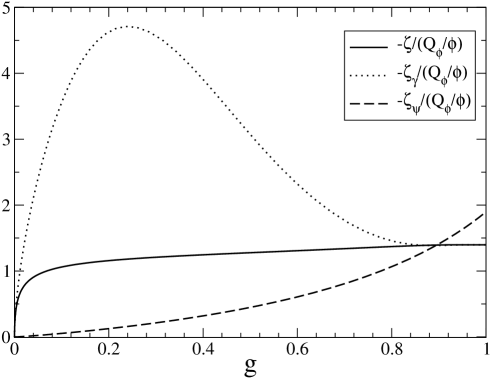
Figure 1: Evolution of $\zeta$, $\zeta_{\psi}$, and $\zeta_{\gamma}$ normalized to the light field perturbation $-{\cal Q}_{\phi}/\phi$, as a function of $g$, for $R_{\rm in}=10$, where we have taken the simplest case where the dependence of $\Gamma$ and $M$ is linear in the field, $M\propto\Gamma\propto\phi$. Although it is not visible on the ($\zeta_{\bullet},g$)-plane, for $g\to 1$ the uniform-density perturbations approach a fixed point attractor.

The behavior of $r$ as a function of $R_{\rm in}$ is illustrated in Fig. 2 and it is obtained by solving numerically Eqs. (55-57).

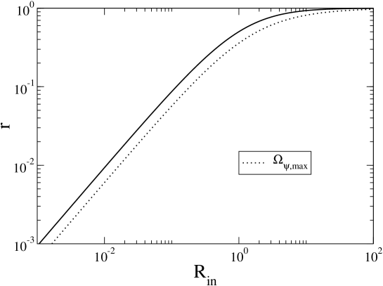
Figure 2: The function $r$, parametrizing the conversion from an isocurvature to a curvature perturbation, as a function of the initial parameter $R_{\rm in}$ (solid line). This is compared to $\Omega_{\psi,\rm max}$ (dashed line), the maximum value reached by $\Omega_{\psi}$ before decaying as a function of $R_{\rm in}=\Omega_{\psi}(H/\Gamma)^{1/2}|_{\rm in}$.

For large $R_{\rm in}$, $r=1$ and the efficiency of the mechanism of conversion of the density perturbation of $\phi$ into a curvature perturbation is simply given by $\alpha_{\phi}$. For small $R_{\rm in}$, $r\ll 1$ and the efficiency is considerably reduced. In Fig. 2 the maximum value reached by $\Omega_{\psi}$ before the decay is also shown. For large $R_{\rm in}$ one can approximate $r$ by this value. Note that $r$ as defined here is the same as the one defined in curvaton4 and computed in wmu for the curvaton model. We numerically checked that this is the case .

We can represent the integration of Eqs. (55-57) as a transfer matrix acting on the initial perturbations,

$$\left(\begin{array}[]{c}\zeta\\ {\cal Q}_{\phi}/\phi\end{array}\right)_{\rm out}=\left(\begin{array}[]{cc}1&-r\alpha_{\phi}\\ 0&1\end{array}\right)\left(\begin{array}[]{c}\zeta\\ {\cal Q}_{\phi}/\phi\end{array}\right)_{\rm in}.$$ (62)

Since the energy density of the light field $\phi$ is always negligible, its perturbation represents an entropy perturbation which is converted into a curvature perturbation if $\alpha_{\phi}$ and $r$ are non-zero. Our task is now to estimate the efficiency parameters $\alpha_{\Gamma}$ and $\alpha_{M}$. Below we discuss two different physical situations.

IV.1 Inhomogeneous inflaton decay

Here we discuss case (A) as mentioned in Sec. II. The oscillating inflaton is described by the fluid $\psi$ and $C_{M}=0$ is used. Although fluctuating, the decay rate of the inflaton is time independent in the limit (44). Initially, the inflaton dominates the universe, $\Omega_{\psi}\to 1$ for $g\to 0$, whereas the radiation is negligible; thus we take $R_{\rm in}\gg 1$ and $r=1$. The initial condition of $\zeta_{\psi}$ is given by the initial perturbation of the inflaton field corresponding to vacuum fluctuations. According to gamma1 we assume that the density perturbation of the inflaton field is negligible. Therefore we have $|{\cal Q}_{\phi}/\phi_{*}|\gg|\zeta_{\psi,\rm in}|=|\zeta_{\rm in}|$, where we have used Eq. (58) with $C_{M}=0$ and $\Omega_{\gamma}=0$ for the last equality, and $\phi_{*}$ is the VEV of $\phi$ at horizon crossing. Solving Eqs. (55-57) with $R_{\rm in}\gg 1$ (inflaton domination) we find $\alpha_{\Gamma}=1/6$. This leads to the result found in gamma1 ; Riotto ; Mazum ; Zalda ,

$$\zeta=-\frac{1}{6}\frac{\delta\Gamma}{\Gamma},$$ (63)

valid on the spatially flat slices $\Psi=0$.

IV.2 Inhomogeneous mass-domination and decay

Here we discuss case (B) as mentioned in Sec. II. Now $\psi$ is the massive particle species and both the mass $M$ and decay rate $\Gamma$ depend on $\phi$. The radiation $\gamma$ is the product of a previous reheating and it initially dominates the universe, $\Omega_{\gamma,\rm in}\simeq 1$.

We start by discussing the condition for the massive particles to dominate the universe before decaying. Assuming that the massive species $\psi$ is sub-dominant when the initial conditions are setup, the initial parameter $R_{\rm in}$ can be written as

$$R_{\rm in}\simeq\left(\frac{M^{2}}{M_{\rm Pl}\Gamma}\right)^{1/2}g_{r}^{1/4}\frac{n_{\psi}}{s},$$ (64)

where $g_{r}$ is the number of relativistic degrees of freedom and $n_{\psi}/s$ is the relic abundance of the $\psi$ particles when they freeze-out ($s$ is the entropy density). In order to derive Eq. (64) we have used KolbTurner

$$\rho\sim\rho_{\gamma}=\frac{\pi^{2}}{30}g_{r}T^{4},\quad s=\frac{2\pi^{2}}{45}g_{r}T^{3}.$$ (65)

After freeze-out and when $\Gamma\ll H$, $n_{\psi}/s$ is constant if $g_{r}$ is constant (which we shall consider throughout). The massive species has time to dominate the universe if $R_{\rm in}\geq 1$, which translates into

$$\Gamma<\frac{M^{2}}{M_{\rm Pl}}g_{r}^{1/2}\left(\frac{n_{\psi}}{s}\right)^{2}.$$ (66)

If $n_{\psi}/s$ is order unity Eq. (1) is recovered. However, it is interesting to try to plug some numbers for the relic abundance in Eq. (66). We make use of the analytic approximation for the relic abundance of long-lived massive particles derived in JGK . At high temperature ($T\gg M$) $n_{\psi}\propto T^{3}$, whereas at low temperature ($T\ll M$) the $\psi$ density is Boltzmann suppressed, $n_{\psi}\propto T^{3/2}\exp(-M/T)$ so that if the particles freeze-out when $T\mathrel{\hbox to0.0pt{\lower 3.0pt\hbox{$\mathchar 536\relax$}\hss}\raise 2.0pt\hbox{$\mathchar 318\relax$}}M$ then the $\psi$ abundance becomes very small. The initial equilibrium abundance is maintained by annihilation of particles and antiparticles with cross section $\sigma_{A}$ which we take to be independent of the energy of the particles. In this case the abundance at freeze-out is JGK

$$\frac{n_{\psi}}{s}\simeq\frac{100}{MM_{\rm Pl}g_{r}^{1/2}\langle\sigma_{A}v\rangle},$$ (67)

where $\langle\sigma_{A}v\rangle$ is the thermal average of the total cross section times the relative velocity $v$. On using this relation, Eq. (64) becomes independent of the mass $M$,

$$R_{\rm in}\simeq\frac{100}{g_{r}^{1/4}}\left(\frac{M_{\rm Pl}}{\Gamma}\right)^{1/2}\frac{M_{\rm Pl}^{-2}}{\langle\sigma_{A}v\rangle}.$$ (68)

This relation holds if the $\psi$-particles are subdominant at the freeze-out. If a more detailed calculation is performed one can see that the mass dependence enters only via a logarithmic correction JGK .

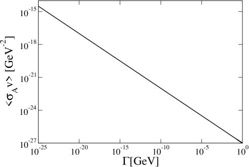
Figure 3: Values of $\Gamma$ and $\langle\sigma_{A}v\rangle$ for which $R_{{\rm in}}=1$. For values below this line the $\psi$-particles come to dominate the universe. We have taken $g_{r}\simeq 100$.

In Fig. 3 we show the values of $\Gamma$ and $\langle\sigma_{A}v\rangle$ for which $R_{\rm in}=1$ and the $\psi$-particles come to dominate. On requiring that the massive particles decay before nucleosynthesis i.e., $\Gamma>(1\ {\rm MeV})^{2}/M_{\rm Pl}$, we find that only for $\langle\sigma_{A}v\rangle<(100/g_{r})^{1/2}(10^{7}{\rm GeV})^{-2}$ does $\psi$ dominate the universe. In this case, the initial thermal equilibrium by annihilation of particles and antiparticles must be maintained by some gauge interaction much weaker than those of the standard model. This excludes $\psi$ as being made by standard model particles.

Let us now discuss the perturbations. The initial perturbation of the radiation is left over by inflation and it is negligible. The species $\psi$ is initially in thermal equilibrium with $\gamma$, $\zeta_{\psi,\rm in}=\zeta_{\gamma,\rm in}$, and Eq. (58) implies ${\cal Q}_{\phi}/\phi_{*}\gg\zeta_{\gamma,\rm in}=\zeta_{\rm in}$. For the value of $\alpha_{M}$ we find numerically $\alpha_{M}=4/3$. Thus, in general for a $\phi$-dependent mass and decay rate

$$\zeta=-r\left(\frac{1}{6}\frac{{\cal Q}_{\Gamma}}{\Gamma}+\frac{4}{3}\frac{{\cal Q}_{M}}{M}\right).$$ (69)

If the massive particles dominate the universe before decaying, i.e., if $R_{\rm in}\gg 1$, $r=1$. For $M=$ constant we recover the result of the inhomogeneous inflaton decay discussed in the preceding section. If the mass depends on $\phi$ while $\Gamma$ does not, we find

$$\zeta=-\frac{4}{3}\frac{{\cal Q}_{M}}{M}.$$ (70)

Finally, if $M\propto\Gamma$ we find

$$\zeta=-\frac{3}{2}\frac{{\cal Q}_{\Gamma}}{\Gamma},$$ (71)

a result nine times larger than the one obtained in the case where only $\Gamma$ is fluctuating.

In Ref. gamma3 the perturbation generated by a varying mass is derived with an analytic argument which yields $\zeta=(1/3)({\cal Q}_{M}/M)$, a result different from the one of Eq. (70). This difference is due to the fact that in our model, specified by the conservation equations (6-8), the entropy perturbation stored in the light field is important. Indeed, when $C_{M}\neq 0$, $\dot{\rho}_{\phi}\neq 0$ and the light field perturbation contributes to the relative non-adiabatic pressure $\delta P_{\rm rel}$ [see Eq. (29)] and sources the evolution of the total curvature perturbation, as shown by Eq. (55).

IV.3 Comparison with the curvaton model

It is worth discussing here the curvaton model, a mechanism of generation of perturbations which has very similar properties as the model discussed here. The aim is to stress their similarities and compare their efficiency. The curvaton $\sigma$ is a scalar field which is practically free during inflation and starts oscillating after inflation (but before nucleosynthesis) during the radiation era when $\Gamma\mathrel{\hbox to0.0pt{\lower 3.0pt\hbox{$\mathchar 536\relax$}\hss}\raise 2.0pt\hbox{$\mathchar 316\relax$}}H\mathrel{\hbox to0.0pt{\lower 3.0pt\hbox{$\mathchar 536\relax$}\hss}\raise 2.0pt\hbox{$\mathchar 316\relax$}}m_{\sigma}$, behaving as a non-relativistic fluid. If during the oscillations it comes (close) to dominate the universe before decaying, its perturbation $\zeta_{\sigma}$ is converted directly into curvature perturbations,

$$\zeta=r\zeta_{\sigma}.$$ (72)

We can write the parameter $R_{\rm in}$ in terms of relevant quantities. If we choose the initial time when the curvaton starts to oscillate, at $H\sim m_{\sigma}$, on using $\rho_{\sigma}\sim m_{\sigma}^{2}\sigma^{2}$ we have, from the definition (54),

$$R_{\rm in}\simeq\frac{\sigma^{2}}{3M_{\rm Pl}^{2}}\left(\frac{m_{\sigma}}{\Gamma}\right)^{1/2}.$$ (73)

If the decay rate is sufficiently smaller than the curvaton mass, the curvaton has the time to dominate the universe before decaying. The conditions for the curvaton domination during its oscillations are

$$\left(\frac{\Gamma}{m_{\sigma}}\right)^{1/4}M_{\rm Pl}\mathrel{\hbox to0.0pt{\lower 3.0pt\hbox{$\mathchar 536\relax$}\hss}\raise 2.0pt\hbox{$\mathchar 316\relax$}}\sigma\mathrel{\hbox to0.0pt{\lower 3.0pt\hbox{$\mathchar 536\relax$}\hss}\raise 2.0pt\hbox{$\mathchar 316\relax$}}M_{\rm Pl},$$ (74)

where the last inequality ensures that the curvaton does not dominate before starting to oscillate.

Equations (55-57) describe the curvaton model if we set $C_{M}=C_{\Gamma}=0$ wmu in which case $\psi$ represents the curvaton during its oscillating phase, with $\zeta_{\psi,\rm in}\equiv\zeta_{\sigma,\rm in}\gg\zeta_{\rm in}$. By considering a massive curvaton we have curvaton2

$$-H\frac{\delta\rho_{\sigma}}{\dot{\rho}_{\sigma}}=\frac{1}{3}\frac{\delta\rho_{\sigma}}{\rho_{\sigma}}=\frac{2}{3}\frac{\delta\sigma}{\sigma}.$$ (75)

For the last equality we have assumed that the field remains overdamped until the Hubble parameter falls below the curvaton mass, which is the case if Eq. (74) is satisfied. Thus, from Eq. (72) we obtain

$$\zeta=r\frac{2}{3}\frac{{\cal Q}_{\sigma}}{\sigma}\equiv-r\alpha_{\sigma}\frac{{\cal Q}_{\sigma}}{\sigma}.$$ (76)

If we want to compare the efficiency of the inhomogeneous reheating with that of the curvaton model we must compare the efficiency parameter $\alpha_{\sigma}=-\frac{2}{3}$ to $\alpha_{\phi}$ in Eq. (59), which varies according to the dependence of the mass and decay rate on the light field $\phi$. However, in the simplest case where $\Gamma\propto M\propto\phi$, $\alpha_{\phi}$ has opposite sign to $\alpha_{\sigma}$ and it is nearly twice as larger.

We end this section with a comment. The physical situations discussed in this section using Eqs. (55-57) assume that the mass of $\phi$ must remain smaller than the Hubble parameter during the whole process of inhomogeneous reheating. However, this relation may be violated during the $\psi$ domination if $m_{\phi}\sim\Gamma$ and $\phi$ starts to oscillate during this period. This leads to a mix situation of curvaton/inhomogeneous reheating scenario, where the perturbation of $\phi$ is converted into a curvature perturbation via both the curvaton mechanism (the curvaton being $\phi$) and the inhomogeneous reheating. Since the sign of the efficiency parameters $\alpha_{\bullet}$ can be different for the curvaton and inhomogeneous reheating models this may lead to a compensation between them. An example of this situation is given in Mazum . The full calculation of the resulting curvature perturbation in the inhomogeneous mass-domination can be done starting from Eqs. (39-43).

V Observational constraint of the model

Here we discuss the observational predictions of the inhomogeneous reheating models: isocurvature perturbations and non-Gaussianities.

V.1 Isocurvature perturbations in the mass-domination mechanism

If the inflaton or the $\psi$-particles decay into species out of equilibrium which remain decoupled from the radiation, we expect isocurvature perturbations to be present into these species. These can be correlated with the adiabatic perturbation. Here we consider the case where the perturbations left over from inflation are of the same order of magnitude as the perturbations produced during the inhomogeneous mass-domination and decay. We define the parameter $\kappa$ to quantify the relevance of the perturbations left over from inflation,

$$\kappa\equiv r\alpha_{\phi}\frac{{\cal Q}_{\phi}/\phi}{\zeta_{\chi}}=r\alpha_{\phi}\frac{V_{,\chi}}{3H^{2}\phi},$$ (77)

where $\chi$ is the inflaton, $V_{,\chi}$ is the derivative of the inflaton potential, and $H$ is the Hubble parameter, all evaluated at horizon crossing during inflation. When $\kappa$ is order unity or smaller, perturbations from inflation are important. For chaotic inflation we have

$$\kappa_{\rm chaotic}\equiv 2r\alpha_{\phi}\frac{M_{\rm Pl}^{2}}{\chi\phi}.$$ (78)

Using an inflaton field which is $\sim 10M_{\rm Pl}$ and an efficiency $r\alpha_{\phi}\sim{\cal O}(1)$ we obtain $\kappa_{\rm chaotic}\sim 0.2M_{\rm Pl}/\phi$ so that perturbations from inflation are important if the VEV of $\phi$ is sufficiently large, $\phi\sim M_{\rm Pl}$.

The following analysis holds also for the curvaton model, although the VEV of the curvaton during inflation should remain smaller than the Planck mass [see Eq. (74)] and generally $\kappa\gg 1$. Thus, in the curvaton scenario it is not likely that the inflaton and curvaton generated perturbations are of the same order. The VEV of the light field $\phi$ does not need to satisfy this constraint. Indeed, as discussed in gamma3 , if one wants to avoid that at high temperature the non-zero density of the $\psi$-particles generates a large thermal mass for $\phi$ – which would make $\phi$ too heavy and would spoil the simplicity of the mechanism – we must require $\phi\sim M_{\rm Pl}$. We are hence motivated to consider the possibility of $\kappa$ being small, at least for chaotic inflation. In this case perturbations from inflation may not be negligible with respect to perturbations from the light field and a mix of the two may survive. Isocurvature perturbations in the curvaton model are discussed in curvaton4 ; GL and in Moroi , although these groups considered a more general set of possibilities than what considered here and in GL ; Moroi they performed a numerical analysis of the CMB data to constrain the curvaton model. Here however we consider a different possibility i.e., that the cold dark matter (CDM) is a relic left over both from the inflaton and the $\psi$ decay.

We write the $\chi$ and $\phi$ quantum perturbations as $\hat{\cal Q}_{\chi}=(H/\sqrt{2k^{3}})\hat{a}_{\chi}$ and $\hat{\cal Q}_{\phi}=(H/\sqrt{2k^{3}})\hat{a}_{\phi}$, where the $\hat{a}_{\alpha}$’s are independent normalized Gaussian random variables, obeying $\langle\hat{a}_{\alpha}({\bf k})\hat{a}_{\beta}({\bf k}^{\prime})\rangle=\delta_{\alpha\beta}\delta({\bf k}-{\bf k}^{\prime})$. After reheating, if the relic product of the inflaton is decoupled from the product of $\psi$, its uniform curvature perturbation is conserved and given by

$$\hat{\zeta}_{{\rm product~{}of~{}}\chi}=\frac{3H^{2}}{V_{,\chi}}\hat{\cal Q}_{\chi}=\hat{a}_{\chi}\zeta_{\chi}.$$ (79)

From Eq. (62) the uniform curvature perturbation of the product of the $\psi$ decay can be written as

$$\hat{\zeta}_{{\rm product~{}of~{}}\psi}=\frac{3H^{2}}{V_{,\chi}}\hat{\cal Q}_{\chi}-\frac{r\alpha_{\phi}}{\phi}\hat{\cal Q}_{\phi}=(\hat{a}_{\chi}-\kappa\hat{a}_{\phi})\zeta_{\chi},$$ (80)

where the first term in the right hand side comes from the initial perturbation and the second from the fluctuations of $\phi$. Note that $\kappa$, according to its definition (77), is scale dependent. We can write it as $\kappa({\bf k})=\kappa_{0}(k/k_{0})^{\Delta n/2}$ where $\kappa_{0}$ is scale free and $k_{0}$ is a reference pivot scale. The spectral index of $\kappa$, $\Delta n$, can be expressed in terms of the difference between the spectral indexes of $\zeta_{\phi}$ and $\zeta_{\chi}$, $\Delta n\equiv n_{\phi}-n_{\chi}$, but here it is considered as a free parameter.

To simplify the discussion we completely neglect the baryons and we concentrate on the CDM isocurvature mode, which is due to the difference between the uniform curvature perturbations of the CDM and radiation (e.g., photons and neutrinos). We start by assuming that both the inflaton and the $\psi$-particles may decay in CDM particles which are out of equilibrium at the temperature at which they are produced. We define $f$ as the fraction of CDM, evaluated just before nucleosynthesis, which is left over from the decay of $\psi$. The rest of the CDM, $1-f$, is a relic of the inflaton decay. Both the inflaton and the $\psi$-particles may decay into radiation. The fraction of radiation that decays from $\psi$ is proportional to the value of $\Omega_{\phi}$ at the decay, which we assume to be $\Omega_{\phi,\rm max}$ defined in Sec. IV.B. We have seen there that this is very close to $r$. If $r\ll 1$, $\psi$ remains negligible before decaying and cannot be responsible for the radiation . However, $\psi$ can generate part of the CDM leading to an uncorrelated isocurvature mode. This is constrained by data: we have $f\kappa_{0}<0.28$ at $95\%$ confidence level. These bounds come from the numerical analysis of the WMAP data made in Vali , which assumes $-0.72\leq\Delta n\leq 1.11$ and $k_{0}=0.05\ {\rm Mpc}^{-1}$. The amount of CDM produced by the decay of $\psi$ can be important only if the $\psi$ generated perturbation is negligible. More interestingly, when $r\simeq 1$, $\psi$ comes to dominate the universe and the totality of the radiation comes from its decay product. In this case the adiabatic and CDM isocurvature perturbations are correlated. The intermediate case, that the radiation left over at nucleosynthesis is created both by the inflaton and by the $\psi$ is not discussed here. Indeed, the radiation thermalizes and it is difficult to express its final perturbation in terms of primordial perturbations.

We thus concentrate on the case $r\simeq 1$. Making use of the notation of Vali (see also AmendolaGordon ), the adiabatic mode is described by the comoving curvature perturbation in the radiation-dominated era, ${\cal R}_{\rm rad}\equiv-\zeta_{\gamma}$, and the isocurvature mode by ${\cal S}_{\rm rad}\equiv 3(\zeta_{c}-\zeta_{\gamma})$, where $\zeta_{\gamma}$ and $\zeta_{c}$ are the uniform curvature perturbations of the radiation (i.e., photons and neutrinos) and of the CDM, respectively. Well in the radiation era they are both constant and can be written as

$${\cal R}_{\rm rad} = (\kappa\hat{a}_{\phi}-\hat{a}_{\chi})\zeta_{\chi},$$ (81)

$${\cal S}_{\rm rad} = 3(1-f)\kappa\hat{a}_{\phi}\zeta_{\chi}.$$ (82)

According to Vali we define the dimensionless cross correlation as

$$\cos\Delta\equiv\left.\frac{\langle{\cal R}_{\rm rad}{\cal S}_{\rm rad}\rangle}{(\langle{\cal R}_{\rm rad}^{2}\rangle\langle{\cal S}_{\rm rad}^{2}\rangle)^{1/2}}\right|_{k=k_{0}}=\frac{|\kappa_{0}|}{\sqrt{1+\kappa_{0}^{2}}},$$ (83)

and the entropy-to-adiabatic ratio as

$$f_{\rm iso}\equiv\left.\left(\frac{\langle{\cal S}_{\rm rad}^{2}\rangle}{\langle{\cal R}_{\rm rad}^{2}\rangle}\right)^{1/2}\right|_{k=k_{0}}=3(1-f)\cos\Delta.$$ (84)

These depend on two parameters, $f$ and $\kappa_{0}$. For large values of $\kappa_{0}$ the adiabatic perturbation is dominated by the perturbation of the light field and the modes are totally correlated ($\cos\Delta=1$) as found in GL . More generally the correlation is positive but can be small if the inflaton perturbation becomes important.

The entropy-to-adiabatic ratio is constrained by data and cannot be too large. We can lower it by decreasing the amount of relic CDM left over from inflation (i.e., by sending $f$ to 1) or by decreasing the amplitude of the light field perturbation, i.e., the amplitude of $\kappa_{0}$. Since a full analysis of the constraints imposed by the data on this model is well beyond the scope of this paper, we just use the $95\%$ confidence level bounds on the isocurvature mode coefficient $f_{\rm iso}$ as a function of $\cos\Delta$ for correlated perturbations as given in Vali (Fig. 1 in this reference) and we show the bounds on $f$ as a function of $\kappa_{0}$ in Fig. 4.

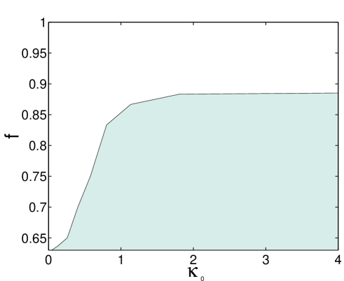
Figure 4: Bounds on $f$, the fraction of CDM created by $\psi$, as a function of $\kappa_{0}\equiv r\alpha_{\phi}{\cal Q}_{\phi}/(\phi\zeta_{\chi})$ at $95\%$ confidence level. The filled region is excluded.

Totally correlated perturbations are allowed only if the CDM is almost completely created by $\psi$ ($f=1$). However, even for $\kappa\gg 1$, $\sim 10\%$ of CDM created by the inflaton is allowed. The signature of a correlated CDM isocurvature mode in the data can be the signal that part of the CDM has been created before the decay of $\psi$. These constraints apply equally well to the curvaton model in the situation discussed here.

V.2 Non-Gaussianities

Until now we have assumed that the density perturbation of the light field $\phi$ depends linearly on ${\cal Q}_{\phi}/\phi$, which we take to be a Gaussian variable. However, when the perturbation ${\cal Q}_{\phi}$ is comparable to the average value $\phi$ – which is the case for small values of $\alpha_{\phi}$ – the non-linear term $({\cal Q}_{\phi}/\phi)^{2}$ can be important and lead to a non-Gaussian $\chi^{2}$ contribution in the spectrum of curvature perturbations gamma3 ; Zalda ,

$$\zeta=-r\alpha_{\phi}\left[\frac{{\cal Q}_{\phi}}{\phi}-\frac{1}{2}\left(\frac{{\cal Q}_{\phi}}{\phi}\right)^{2}\right].$$ (85)

The level of non-Gaussianity is conventionally specified by the non-linear parameter $f_{\rm NL}$ Kamiol ; KomaSper . We can write the total uniform curvature perturbation as Criminelli

$$\zeta=\zeta_{g}-\frac{3}{5}f_{\rm NL}\zeta_{g}^{2},$$ (86)

where $\zeta_{g}$ represents the Gaussian contribution to $\zeta$. Using Eq. (85) the prediction for the inhomogeneous reheating is

$$f_{\rm NL}=-\frac{5}{6r\alpha_{\phi}},$$ (87)

which is the same as for the curvaton scenario once the replacement $\alpha_{\phi}=-2/3$ of Eq. (76) is used. However, Eq. (87) has to be taken with caution: In order to precisely estimate the non linear parameter $f_{\rm NL}$ generated by these models one has to study and solve the second order perturbation equations as done in RiottoBartolo and find the second order correction to Eq. (69).

If we use Eq. (87) we see that less efficiency in the mechanism of conversion of perturbations means more non-Gaussianities in the spectrum. If detected non-Gaussianity could be the smoking-gun of models where perturbations are produced with an ‘inefficient’ mechanism of conversion. The WMAP experiment has now put a limit on $f_{\rm NL}$ corresponding to $-58<f_{\rm NL}<134$ at the $95\%$ level WMAP4 , which already excludes models with $-0.006<\alpha_{\phi}<0.014$. Planck will put a more sever constraint, $|f_{\rm NL}|\mathrel{\hbox to0.0pt{\lower 3.0pt\hbox{$\mathchar 536\relax$}\hss}\raise 2.0pt\hbox{$\mathchar 316\relax$}}5$ KomaSper , corresponding to $|\alpha_{\phi}|\mathrel{\hbox to0.0pt{\lower 3.0pt\hbox{$\mathchar 536\relax$}\hss}\raise 2.0pt\hbox{$\mathchar 318\relax$}}1/6$.

Going back to the inhomogeneous reheating, in which the mechanism of conversion of the density perturbation of $\phi$ into a curvature perturbation is due to the fluctuations of the decay rate and $\Gamma\propto\phi$ we have $r\alpha_{\phi}\leq 1/6$ and the non-Gaussianity can be large, $-5\leq f_{\rm NL}<0$. In particular, if the non-relativistic species $\psi$ completely dominates the universe before decaying ($r=1$) $f_{\rm NL}=-5$ gamma3 , a value which is right in the ball-park of Planck observations. However, the inhomogeneous mass-domination can be much more efficient. If $M\propto\Gamma\propto\phi$, $r\alpha_{\phi}\leq 3/2$ and thus $-5/9\leq f_{\rm NL}<0$. If the massive species dominates completely the universe before decaying ($r=1$) we have $f_{\rm NL}=-\frac{5}{9}$, a much smaller value than the one estimate in gamma3 and not observable by future planned experiments.

VI Conclusion

In this paper we have studied the evolution of perturbations during a phase dominated by massive particles whose mass and decay rate can fluctuate in space and time. If the fluctuations are set by the VEV of a light scalar field overdamped during inflation, the isocurvature perturbation in the scalar field can be converted into a curvature perturbation, and this can be the main mechanism of generation of large scale perturbations for structure formation. We have derived a set of perturbation equations that can be used in full generality for any kind of dependence of the mass and decay rate on the light field. Making use of these perturbation equations we have recovered the results of gamma1 ; Riotto ; Mazum for the inhomogeneous reheating with varying decay rate. We have also discussed the condition for the massive particles to dominate the universe before decaying. This condition does not depend on their mass, but depends on the annihilation cross section and decay rate. Standard model massive particles cannot dominate the universe. Furthermore, we have shown that when the mass of the massive particles is allowed to vary, the mechanism of conversion can be nine times more efficient. The final total curvature perturbation is $\zeta=-(1/6)\delta\Gamma/\Gamma-(4/3)\delta M/M$. This is our main result. Finally, we have compared this with the curvaton model discussing differences and similarities.

On the observational side we have discussed two possible signatures of the mass-domination mechanism: correlated adiabatic and isocurvature perturbations and non-Gaussianities. If present, a cold dark matter isocurvature perturbation provides some important information on the mechanism of generation of the dark matter and on the vacuum expectation values of the inflaton and light field during inflation. There are non-Gaussianities generated by this mechanism, which are $\chi^{2}$. In order to precisely compute them one has to study the evolution of second order perturbations. In the limit where $f_{\rm NL}$ is large, by simply using Eq. (87) the non-linear parameter is $f_{\rm NL}=-5/(6r\alpha_{\phi})$. When both the mass and the decay rate of the massive particles fluctuate, due to the high efficiency the non-Gaussianities can be much smaller than what is possibly observable, $f_{\rm NL}\ll-5$.

Acknowledgment

It is a pleasure to thank Roberto Trotta for very fruitful discussions and suggestions. I also acknowledge Ruth Durrer, David Langlois, Karim Malik, and Jean-Philippe Uzan for very helpful suggestions and comments, Robert Brandenberger for carefully reading the manuscript, and Nicola Bartolo, Antonio Riotto and Sabino Matarrese for drawing my attention on the importance of the evolution of second order perturbations. Part of this work was done at the Kavli Institute of Theoretic Physics. This research was supported in part by the National Science Foundation under Grant No. PHY99-07949 and by the Swiss National Science Foundation.

References

- (1) C. L. Bennett et al., Astrophys. J. Suppl. Ser. 148,1 (2003).
- (2) D. N. Spergel et al., Astrophys. J. Suppl. Ser. 148, 175 (2003).
- (3) H. V. Peiris et al., Astrophys. J. Suppl. Ser. 148, 213 (2003).
- (4) E. Komatsu et al., Astrophys. J. Suppl. Ser. 148, 213 (2003).
- (5) G. Hinshaw et al., Astrophys. J. Suppl. Ser. 148, 135 (2003).
- (6) A. Guth, Phys. Rev. D 23, 347 (1981).
- (7) V. F. Mukhanov, H. A. Feldman and R. H. Brandenberger, Phys. Rept. 215 203 (1992).
- (8) K. Enqvist and M. S. Sloth, Nucl. Phys. B 626, 395 (2002).
- (9) D. H. Lyth and D. Wands, Phys. Lett. B 524, 5 (2002).
- (10) D. H. Lyth, C. Ungarelli and D. Wands, Phys. Rev. D 67, 023503 (2003).
- (11) T. Moroi and T. Takahashi, Phys. Lett. B 522, 215 (2001) [Erratum-ibid. B 539, 303 (2002)] [arXiv:hep-ph/0110096].
- (12) G. Dvali, A. Gruzinov and M. Zaldarriaga, Phys. Rev. D 69, 023505 (2004).
- (13) L. Kofman, [arXiv:astro-ph/0303614].
- (14) M. S. Turner, Phys. Rev. D 28 1243 (1983).
- (15) K. Enqvist, A. Mazumdar, and M. Postma, Phys. Rev. D 67, 121303 (2003).
- (16) G. Dvali, A. Gruzinov and M. Zaldarriaga, [arXiv:astro-ph/0305548].
- (17) S. Matarrese and A. Riotto, JCAP 0308, 007 (2003).
- (18) A. Mazumdar and M. Postma, Phys. Lett. B 1573, 5 (2003).
- (19) S. Tsujikawa, Phys. Rev. D 68, 083510 (2003).
- (20) M. Zaldarriaga, Phys. Rev. D (to be published) [arXiv:astro-ph/0306006].
- (21) K. A. Malik, D. Wands and C. Ungarelli, Phys. Rev. D 67, 063516 (2003).
- (22) H. Kodama and M. Sasaki, Prog. Theor. Phys. Suppl. 78 1 (1984).
- (23) T. Hamazaki and H. Kodama, Prog. Theor. Phys. 96 1123 (1996).
- (24) T. Damour, G. W. Gibbons and C. Gundlach, Phys. Rev. Lett. 64, 123-126 (1990); T. Damour and A. M. Polyakov, Nucl. Phys. B 423, 532 (1994); Gen. Rel. Grav. 26, 1171 (1994).
- (25) G. R. Farrar and P. J. Peebles, [arXiv:astro-ph/0307316].
- (26) D. F. Mota, J. D. Barrow, [arXiv:astro-ph/0309273]; ibid. Phys. Lett. B 581, 141 (2004).
- (27) J. Khoury and A. Weltman, [arXivastro-ph/0309300]; ibid. Phys. Rev. D (to be published) [arXiv:astro-ph/0309411].
- (28) L. Amendola, Phys. Rev. D 62, 043511 (2000); L. Amendola and D. Tocchini-Valentini, Phys. Rev. D, 66, 043528 (2002); S. Matarrese, M. Pietroni, and C. Schimd, JCAP 0308, 005 (2003).
- (29) J. M. Bardeen, Phys. Rev. D 22, 1882 (1980).
- (30) J. M. Bardeen, P. J. Steinhardt and M. S. Turner, Phys. Rev. D 28, 679 (1983).
- (31) D. Wands, K. Malik, D. H. Lyth, and Andrew R. Liddle, Phys. Rev. D 62, 043527 (2000).
- (32) J. García Bellido and D. Wands, Phys. Rev. D 53, 5437 (1996).
- (33) M. Sasaki, Prog. Theor. Phys. 76, 1036 (1986); V. F. Mukhanov, Zh. Éksp. Teor. Fiz. 94, 1 (1988) [Sov. Phys. JETP 52, 807 (1988)].
- (34) C. Gordon, D. Wands, B. A. Basset, and R. Maartens, Phys. Rev. D 63, 023506 (2000).
- (35) E. W. Kolb and M. S. Turner, “The early universe”, (Addison-Wesley Reading Mass., 1990).
- (36) G. Jungman, M. Kamionkowski, K. Griest, Phys. Rep. 267, 195-373 (1996).
- (37) C. Gordon and A. Lewis, Phys. Rev. D 67, 123513 (2003).
- (38) T. Moroi and T. Takahashi, Phys. Rev. D 66, 063501 (2002).
- (39) N. Bartolo, S. Matarrese, and A. Riotto, Phys. Rev. D 65, 103505 (2002).
- (40) J. Valiviita and V. Muhonen, Phys. Rev. Lett. 91, 131302 (2003).
- (41) L. Amendola, C. Gordon, D. Wands, M. Sasaki, Phys. Rev. Lett. 88, 211302 (2002).
- (42) L. Verde, L. Wang, A. F. Heavens, and M. Kamionkowski, MNRAS 313, 141 (2000).
- (43) E. Komatsu and D. N. Spergel, Phys. Rev. D 63, 063002 (2001).
- (44) P. Criminelli, JCAP 10, 003 (2003).
- (45) N. Bartolo, S. Matarrese, and A. Riotto, Phys. Rev. D (to be published) [arXiv:hep-ph/0309033]; ibid. JCAP 01, 003 (2004).