NGC 2264 IRS1: the central engine and its cavity

Abstract

We present a high–resolution study of NGC 2264 IRS1 in CS 2$\rightarrow$1 and in the 3-mm continuum using the IRAM Plateau de Bure Interferometer. We complement these radio data with images taken at 2.2 $\mu$m, 4.6 $\mu$m, and 11.9 $\mu$m. The combined information allow a new interpretation of the closest environment of NGC 2264 IRS1. No disk around the B–type star IRS1 was found. IRS1 and its low–mass companions are located in a low–density cavity which is surrounded by the remaining dense cloud core which has a clumpy shell–like structure. Strong evidence for induced on–going star formation was found in the surroundings of IRS1. A deeply embedded very young stellar object 20^′′ to the north of IRS1 is powering a highly collimated bipolar outflow. The object 8 in the closer environment of IRS1 is a binary surrounded by dusty circumbinary material and powering two bipolar outflows.

1 Introduction

The near–infrared source NGC 2264 IRS1 (IRAS 06384+0932, Allen 1972) is a relatively isolated luminous infrared source (distance 800 pc) in the star–forming region NGC 2264. Previous observations (Schwartz et al., 1985; Krügel et al., 1987; Phillips et al., 1988; Schreyer et al., 1997) suggest that IRS1 is a young star located within a dense molecular core. This core is embedded in a more extended CO envelope. The 2–200 $\mu$m luminosity of $\approx$ 3500 L_⊙ (Harvey, Campbell, & Hoffman, 1977) implies an early B–type zero–age main–sequence star (Schwartz et al., 1985).

Previous ground–based near–infrared images (Scarrott & Warren–Smith 1989; Schreyer et al. 1997) show a twisted jet–like feature to the north of NGC 2264 IRS1, which could be a gas stream “piercing” the surrounding dark cloud. Two outflow systems were reported in this region (Schreyer et al., 1997), one at the position of IRS1 and a second one associated with a deeply embedded small star cluster $\approx 47^{\prime\prime}$ to the southeast of IRS1. Ward–Thompson et al. (2000) found a ridge (NGC 2264 MMS) of bright submm- and mm–emission around IRS1 wherein five emission peaks (MMS 1–5) are located. MMS 3 is associated with the gas clump at the position of the small star cluster (Schreyer et al., 1997) MMS 4 and 5 are located on the eastern and southern side of IRS1, respectively. Wang et al. (2002) found a number of bipolar jets in the region of NGC 2264 MM which point to complex star formation processes in the whole area (diameter $\leq 2^{\prime}$). The high resolution H¹³CO⁺ 1$\rightarrow$0 map of Nakano, Sugitani, and Morita (2003) shows a shell of dense gas clumps around IRS1. Their corresponding continuum map displays four more compact millimeter sources, three in the closer surroundings of IRS1, and one is associated with the small star cluster to the southeast (MMS3).

In this paper^,, we focus on the infrared source IRS1 and its nearest environment (diameter $\leq 51^{\prime\prime}$). We studied this region in the $K$(2.2$\mu$m)–band with ESO’s NTT as well as in the CS 2$\rightarrow$1 line and the 3-mm continuum using the Plateau de Bure Interferometer (PdBI). Additional thermal infrared data came from observations with ESO’s mid-infrared camera TIMMI2. The aim of this study was to answer the following questions: What is the reason for the displaced centre of the bipolar outflow seen with single–dish telescopes (e.g. Schreyer et al. 1997)? Does the presence of a “wiggled jet” possibly originating from IRS1 imply the existence of a disk around IRS1 ? Is this twisted jet dense enough to be traced with the PdBI in order to obtain some information about the velocity structure? Is there an opposite “jet–like” feature  to confirm the suggestion of a (bipolar) jet? Finally, we wanted to learn what the nature of the central engine is.

2 Observations

Near–infrared images of NGC 2264 IRS 1 were obtained with SOFI at ESO’s New Technology Telescope (NTT) on 1999 March 3 in the Ks band. These observations were performed in polarization mode, i.e., with the Wollaston prism and a slit mask at a pixel scale of 0$\farcs$295. After standard image processing (flat–fielding, sky removal and bad–pixel correction) the total intensity image resulted from the co–addition of four frames taken at polarizer orientations of 45${}^{\circ}\!\!,$ 90${}^{\circ}\!\!,$ 135${}^{\circ}\!\!,$ and 180${}^{\circ}\!\!.$ The total integration time amounts to 384 seconds. The observing conditions were very good, leading to a FWHM of the stellar images of 0$\farcs$57. Furthermore, for the central overlap region of the stripes (covering IRS1 and its near vicinity) these data were used to deduce a polarisation map.

Imaging at 11.9$\mu$m (pixel scale 0$\farcs$202) and 4.6 $\mu$m (pixel scale 0$\farcs$315) was performed on 2001 March 18 with TIMMI2 (Reimann et al., 2000) at ESO’s 3.6-m telescope. Chopping was done perpendicular to nodding; the offset throw for both movements was 20^′′ at 11.9$\mu$m and 30^′′ at 4.6 $\mu$m, respectively. We restored the original field of view by applying the Projected Landweber restoration method (Bertero, Boccacci, & Robberto 2000) to the data, which we modified for our purposes (see Linz et al. 2003).

With the PdBI (Guilloteau et al., 1992), we observed CS 2$\rightarrow$1 as well as the corresponding continuum emission at 97.98 GHz. Successful observations were obtained with five 15-m antennas in August and November 1998 using baseline lengths between 21–254 m. We applied one correlator unit with a total bandwidth of 10 MHz centred at the CS 2$\rightarrow$1 line (v_lsr = +8.0 km s^-1) which leads to a velocity resolution of 0.12 km s^-1 ($\widehat{=}$ 0.039 MHz). Two spectral correlator units, each with a bandwidth of 160 MHz, were assigned to the measurements of the continuum. The band pass and phase calibration was performed with the objects 3C454.3, 0528+134, and 0748+126. Compelled by a flux loss of $\approx$50–80% in the PdBI CS 2$\rightarrow$1 data compared to our previous IRAM single-dish data (Schreyer et al. 1997), we combined our IRAM 30-m CS 2$\rightarrow$1 map (extent = 2${}^{\prime}\times$ 2^′ = twice as large as the PdB primary beam) and the PdB interferometer data in order to fill up information about the missing flux between that zero-spacing and the shortest spacing from the interferometer. The IRAM map was Fourier–transformed and then fiddled into the PdB visibility data. Hereby, we benefit from the fact, that the diameter of the single-dish telescope (30 m) is twice as large as the one of the interferometer telescopes (15 m), and that we have also included short baselines (down to 21 m) for the interferometer measurements. Thus, regarding the density of uv points, there is a relatively smooth transition from the contribution of the single-dish data to the contribution of short–baseline interferometer data. With the visibilities resulting from the Fourier–transformed single–dish map we completely cover the uv points of the shortest PdB baseline. Maps of 256$\times$256 square pixels with 0.5^′′ pixel size were produced by Fourier–transforming the calibrated visibilities, using natural weighting. The synthesized beam sizes (HPBW) are 3.05^′′$\times$1.82^′′ for the continuum data and 3.21^′′$\times$1.95^′′ for the line map (with zero–spacing correction), each with a position angle of 21${}^{\circ}\!\!.$ For the data reduction and the final phase calibration, we used the Grenoble Software environment GAG.

3 Results and data analysis

3.1 Infrared results

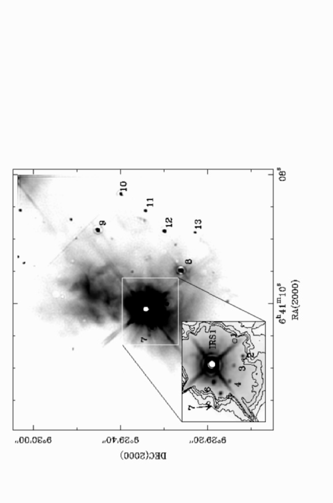
Figure 1: The NTT $K$–band image, whereby the large image is shown with very low cuts to emphasize fine details, e.g., the zig–zag structure to the northwest. The contour lines are 0.11%, 0.15%, 0.19%, and 0.23% of the peak value.

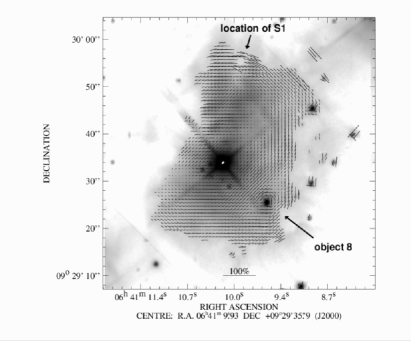
Figure 2: The $K$–band polarisation map in the region around IRS1. Object 8 shows its own centrosymmetric polarization pattern, confirming that this object is surrounded by circumstellar dust. Note the decrease in intensity at the location of the mm–continuum source S1 (see Fig. 5) which also causes a localised disruption of the polarisation pattern.

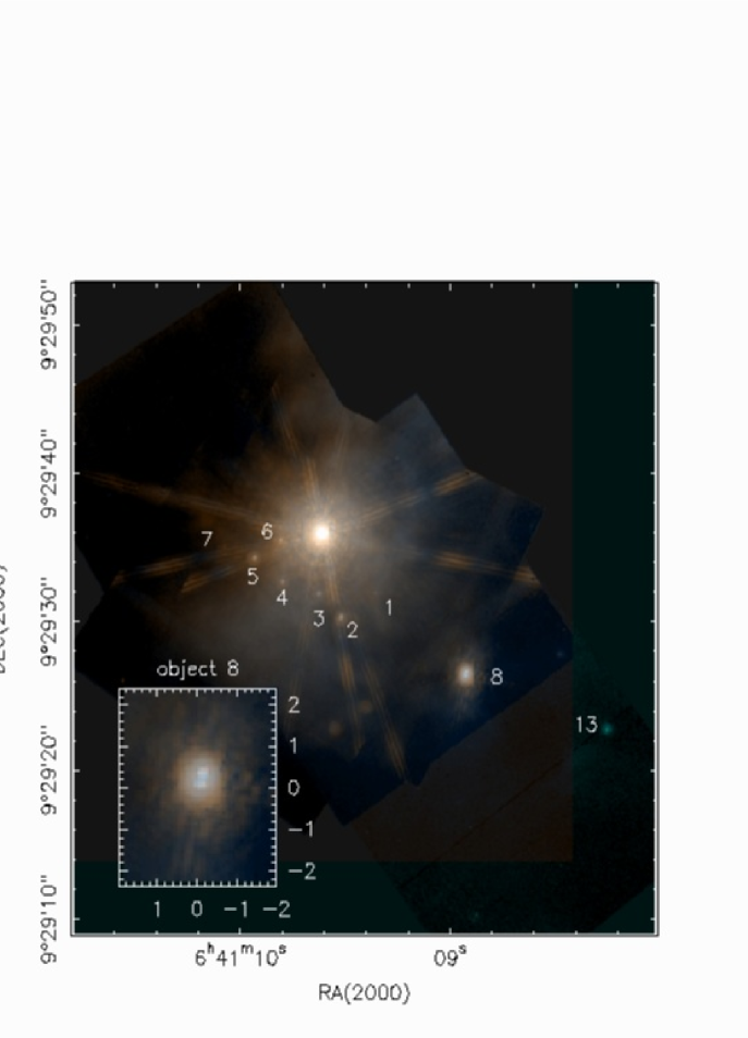
Figure 3: The NICMOS mosaic image is composed of the following three images: the 1.6-micron image (blue), the mean of 1.6-micron and 2.2-micron images (green), and the 2.2-micron image (red).

Fig. 1 and Fig. 2 show the NTT $K$–band image and the $K$–band polarisation map, respectively. The six low–mass companions to the south of IRS1 coincide with the faint objects shown in the HST NICMOS image obtained by Thompson et al. (1998) who labeled these as object 1 to 6. An additional very faint object 7 was found (see Table 1) which was not recognized by Thompson et al. since it was close to the diffraction spikes in the NICMOS images. The other most intense $K$–band stars, seen in the NTT image, are denoted with 8 to 13. Object 8 seems to be of special interest since it is not point–like but marginally extended in the NS direction. While the overall polarization is caused by scattered light from IRS 1, object 8 shows its own centrosymmetric polarization pattern (see Fig. 2), confirming that this object is surrounded by circumstellar dust. Thus, we identify object 8 as an young stellar object in the immediate vicinity of IRS 1. This result is confirmed by archival NICMOS images taken for testing the coronograph (Proposal ID. 7808). Fig. 3 is a composite we constructed from these NICMOS images which shows that object 8 is a binary. The projected separation of the two components amounts to 0.27^′′$\pm$0.01^′′ (= 216 AU) which is somewhat larger compared to the GG Tau binary system with a projected separation of 38 AU. In addition, the faint object 7 is present in this figure.

The NTT image exhibits a similar jet–like feature – as found in the previous low–resolution images by Hodapp (1994) and Schreyer et al. (1997) – which looks like a twisted gas stream to the north of IRS1. However, both, the NTT and the NICMOS images do not clarify the true origin of this feature. We note that, based on the images alone, the illuminated features to the north could be also material which ablates from the surface of a denser cloud clump behind IRS1.

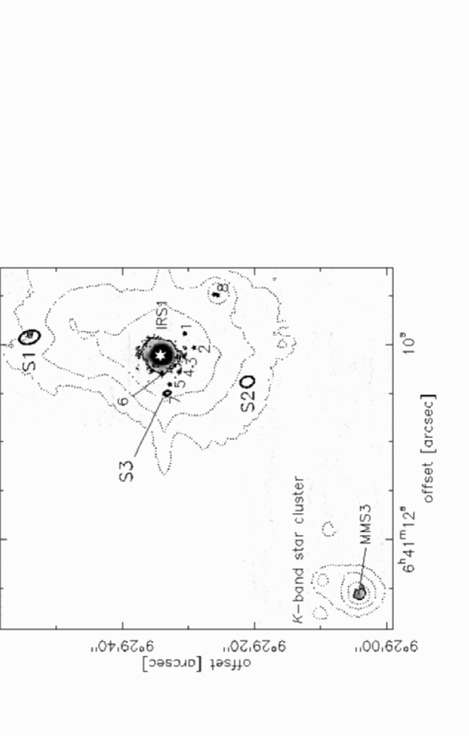
Figure 4: The TIMMI2 image at 11.9 $\mu$m (grey-scale image) with 6$\sigma$ and 8$\sigma$ (thin black) contour lines is overlaid with the thick 50% contours (ellipses) of the 3mm-continumm point sources S1, S2 and S3 (see Sect. 3.3), and the dotted contours of the $K$-band image of Schreyer et al. (1997). The three 11.9 $\mu$m sources correspond to IRS1, S1, and MMS3.

With TIMMI2 we find three sources at 11.9 $\mu$m in the restored field of view (Fig. 4). We detect IRS1 itself as well as the most luminous member of the small star cluster $\approx 47^{\prime\prime}$ southeast of IRS1 (Schreyer et al., 1997). Since both sources have counterparts at 2.2 $\mu$m, we can adopt the near–infrared astrometry for the restored TIMMI2 image. In doing so, we find that the third weak infrared source at 11.9 $\mu$m is located at the position of mm–source S1 (see Sect. 3.3). Since we used the default chopping throw of $20^{\prime\prime}$ in north–south direction, the S1 counterpart is unfortunately placed very near to IRS1 in the chopped and nodded raw image. Although we could recover its true position by applying our image restoration algorithm, the photometric information is strongly affected, so we will not report a photometry here. At 4.6 $\mu$m we did not detect the S1 counterpart which speaks for a deeply embedded object. However, we clearly detect the NIR object 8 also at 4.6 $\mu$m which further increases the reliability of our thermal infrared astrometry. But more important, this detection reveals a clear infrared excess for object 8, which provides strong evidence for dusty circumstellar (or circumbinary) material very near the related young stellar object(s).

3.2 CS $J$ = 2$\rightarrow$1 data

Fig. 5 shows the results of the PdBI measurements. The total integrated CS 2$\rightarrow$1 line emission (continuum subtracted and zero–spacing corrected, contour levels $\geq$50% of the peak emission, Fig. 5a) is overlaid with the NTT image for a better comparsion of the $K$–band objects. CS emission with more than 30% of the peak fills the entire area of the primary beam. The CS map implies that IRS1 is located in a low–density cavity surrounded by denser gas clumps which are possibly cut by the extent of the primary beam. This morphology is in a good agreement with the H¹³CO 1$\rightarrow$0 data obtained by Nakano et al. (2003). If we assume that IRS1 is located in the cavity centre then the mean diameter of the cavity is $\approx 25^{\prime\prime}$ ($\widehat{=}\;2\times 10^{4}$ AU) which matches the extent of the $K$–band nebulosity. Thus, some of the dark cloud clumps are partly located in front or behind the cavity. However, the turbulence inside the clouds is too large in order to find hints from their spectra about the true spatial locations. Both the north- and the southeastern clumps (MMS 4 B/C and MMS 5 A/B/C see Fig. 5a) coincide with the more extended continuum emission peaks MMS 4 and 5 detected by Ward–Thompson et al. (2000) and have counterparts in H¹³CO (Nakano et al. 2003: MMS5 = HC1 + HC2, MMS4 = HC3 + HC4). However, the CS clump MMS 4A shows no well–defined counterpart neither in the data of Ward–Thompson et al.  nor in the data of Nakano et al. At the position of IRS1, no dense gaseous disk was found. Only a small gas clump (MMS 4D) was detected between the positions of IRS1 and the low–mass ‘object 3’ which could be the place of the origin of the twisted gas stream. However, the uncertainty of the overlay positions of $\approx$2^′′ makes it impossible to clarify the true association.

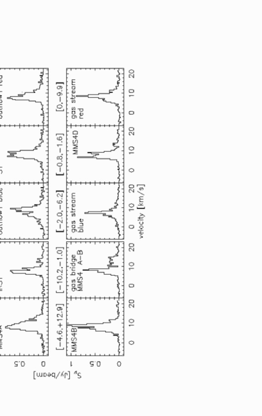
Figure 6: CS 2$\rightarrow$1 spectra taken from different map positions. The corresponding offset position in arcseconds is given in brackets at the top of each spectrum.

The study of the entire data cube implies that the dynamics of the gas in the observed sky region is very complex. In Sect. 3.4, we will report different outflow systems and gas streams in much more detail. Fig. 6 displays selected spectra of different map positions. It is not clear, however, if the CS line is subsequently absorbed, or the spectra present a number of optically thin velocity components. The shape of the spectra varies strongly from position to position. In the observed area, there are hints that the emission at the peak positions of the denser cloud clumps can be absorbed (Fig. 6: MMS 4A, IRS1, S1). However, at other selected positions, e.g. the gas of the twisted $K$–band feature (see Sect. 3.4, map in Fig. 5d, and spectra in Fig. 6: gas stream blue, red), the emission appears to be optically thin.

We estimated the gas mass of the dense cloud fragments inside the 50% contour level applying the formula (2) given by Nakamura et al. (1991). Although the assumptions of LTE and an optically thin CS line emission are not met in our case, we can obtain a lower mass limit using a kinetic temperature of 20 K and a CS abundance of 10${}^{-9}\!\!.$ Table 2 summarises the integrated line emissions and the gas masses for several cloud clumps. Although we cover slightly differnet sky areas for the different cloud clumps, the mass estimates agree well with the results found by Nakano et al. (2003) for the more extended continuum emission as well as for the H¹³CO⁺ measurements.

3.3 Continuum Sources

Three rather weak 3-mm continuum point sources above the 3$\sigma$ level (S1, S2, and S3, see Fig. 5b) were detected. The coordinates of the point sources are listed in Table 1 and agree well with the peaks of the more extended continumm emission regions MC1 (peak S1), MMS4 (peak S2), MMS5 (peak S3) by Nakano et al. (2003). The PdB interferometer did not trace the more extended mm–emission seen by Ward–Thompson et al. (2000) and Nakano et al. (2003). The total integrated continuum fluxes are 8.2 mJy, 4.0 mJy, and 1.4 mJy, and the peak fluxes amount to 9.5, 6.4, and 5.1 mJy beam${}^{-1}\!\!,$ respectively. Neither of these sources is coincident with IRS1. The strongest mm–source S1 is located 20^′′ to the north. If we assume that the overlay positions are correct then the weakest mm–source S3 is associated with the faint $K$–band object 7 in the NTT image.

Using a standard mass derivation algorithm as described by Henning et al. (2000), we estimated gas masses of 3.5 M_⊙ for S1, 1.8 M_⊙ for S2, and 0.6 M_⊙ for S3, using a dust temperature of 20 K, a distance of 800 pc, a gas–to–dust mass ratio of 150, and a mass absorption coefficient of $\kappa^{\rm d}_{\rm m}$ = 0.2 cm² g^-1 (Ossenkopf & Henning 1994: thin icy mantles, gas density of 10⁶ cm^-3), and a density gradient $\propto r^{-2}$.

3.4 Outflows and gas streams

The CS lines show subsequently rather strong and broad line wings. Fig. 5c displays the results of the mapped red– and blue–shifted line wings which shows a more complicated structure. The highly collimated bipolar outflow (outflow 1) to the north of IRS1 whose probable driving source S1 we have detected in the 3-mm continuum as well as at 11.9 $\mu$m is very remarkable. The blue outflow lobe seems to be stopped or redirected into our line of sight very close to IRS1. The outflow masses of the blue (and the mapped part of the red) flow were estimated using the integrated CS intensities $\geq$ 3 $\sigma$ which corresponds to the 30% level contour of the map peaks. The blue flow contains 4.6 10^-3 M_⊙ and the mapped red part 2.5 10^-3 M_⊙. For comparison, we estimate the masses traced with the CS 5$\rightarrow$4 JCMT measurements (Schreyer et al. 1997): both the blue and red components contain 0.2 M_⊙, indicating that the interferometer data trace only the densest flow parts. The estimation of the dynamical flow age is in this case not possible, since the blue flow is redirected and the red flow is cut by the primary beam.

Two bipolar outflows 2a and 2b are produced by the binary object 8 with an angle between them of $\approx$62^∘ in the sky plane. The outflow 2a is, however, much more intense than the outflow 2b. The peaks of the red– and blue–shifted CS emission of outflow 2a are roughly 8–10^′′ (projected distance = 6–8 10³AU) away from the central object. Since the red lobe of the outflow 2b is rather short and ceases near IRS1, we speculate that the binary object 8 can be located in front of IRS1. A third outflow (outflow 3) is associated with the infrared object 9. Based on the number of outflows around IRS1, we can conclude that in the whole observed region around IRS1, the star–forming process is still on–going. With our images, we detect the true baby stars which are not the objects in the HST image presented by Thompson et al (1998).

The morphology of these outflows implies that IRS1 is not the origin of the bipolar outflow always detected with previous single–dish observations.

Fig. 5d shows two CS channel maps. One of the channel maps shows that the twisted jet–like $K$–band feature arising close to IRS1 has a counterpart in the CS gas in a very narrow velocity range between 7.34 and 7.89 km s^-1 which fits very well the “zig–zag” structure of the gas stream. An opposite jet–like feature may be present in the second channel map. However, this gas pours into a denser cloud region. Thus the red–shifted gas stream is not so well separated as the blue–shifted one. Both channel maps clarify that the gas streams present undisturbed gas flows. The twisted shape may be produced by a precession of the central star. Based on the position uncertainties of the overlay, it is not really clear if IRS1 or the infrared object 3 is the origin of the bipolar gas stream or if there is a third obscured object between both sources. In addition, Fig. 5c shows a blue–shifted gas blob at the “end” of the infrared gas stream which seems to be produced by the piercing of the covering dark cloud.

4 Conclusions

We can conclude that IRS1 is in a more evolved evolutionary state than the young B–type objects AFGL 490 (Schreyer et al., 2002) or G192.16–3.82 (Shepherd, Claussen, & Kurtz 2001) which show strong evidence for disks. These results showed that massive accretion disks orbiting B2–3 stars in the first 10³–10⁵ yrs of their main–sequence lifetime exist. However, these disks are unstable and might disappear, for instance, due to gravitational instabilities (e.g., Schreyer et al. 2002). IRS1 seems to be in this phase where the accretion disk already disappeared and a small cavity was created, although, the star is still embedded in the centre of a more extended cloud core (Krügel et al., 1987; Schreyer et al., 1997). The power of IRS1 leads to induced star formation in the surrounding denser cloud clumps, where a number of young stellar objects are embedded powering bipolar outflows. Our data show that the main source of the large-scale bipolar outflow is a deeply embedded young stellar object 20^′′ to the north of IRS1. In addition, the object 8 in the closer environment of IRS1 is a binary surrounded by dusty circumbinary material and powering two bipolar outflows.

Table 1: Positions of the new detected sources. The position of IRS1 (NICMOS) corresponds to Thompson et al. (1999).

object	RA($J$2000)	DEC($J$2000)
	(  h  :  m  :  s)	(  ∘  :  ′  :  ′′)
	[$\pm$0.1s]	[$\pm$0.5′′]
IRS1 (NICMOS)	06:41:10.1	09:29:34.0
object 7	06:41:10.5	09:29:33.2
S1	06:41:09.9	09:29:53.8
S2	06:41:10.5	09:29:33.0
S3	06:41:10.4	09:29:20.9
C1	06:41:12.5	09:29:03.9

Table 2: Integrated CS fluxes and mass estimates for different cloud clumps labeled in Fig. 5a.

cloud clumps	MMS 4A	MMS 5A	MM 4B/C/D	MMS 5A/B/C
$\int$$F$dv [Jy km s-1]	127.33	32.16	184.25	94.77
mass [M⊙]	18.0	4.5	26.0	13.4

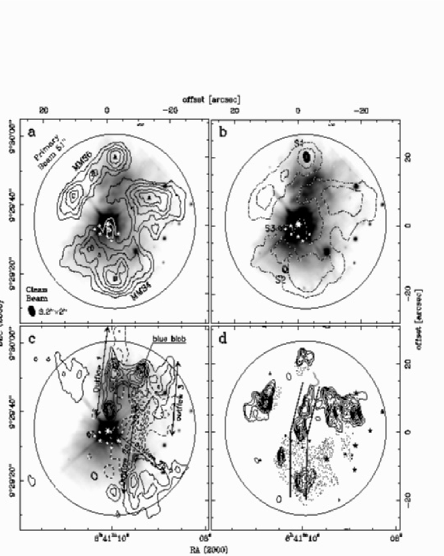
Figure 5: The PdBI data overlaid with the NTT $K$–band image, whereby the image is shown with different lower cut levels to emphasise different cloud structures of the background. The diameter of the primary beam is always indicated with a large circle. a The total integrated CS 2$\rightarrow$1 line emission map (continuum subtracted and zero–spacing corrected, levels: 50% to 90% of the emission peak). The size of the clean beam is shown in the lower left corner. b The three 3-mm continuum sources (levels: 50% to 90% of the peak) are shown with solid contours. The dotted lines indicate the 50% and 70% contours of the total integrated CS line emission of Fig. a. c Integrated CS 2$\rightarrow$1 line wing emissions (red–shifted: 10.8$\leq$v_lsr$\leq$20 km s^-1$\!\!\!,$ dashed contours; blue–shifted: –3.4$\leq$v_lsr$\leq$5.2 km s^-1$\!\!\!,$ solid contours) and the three continuum sources (thick ellipses = 50% contour) are superimposed. d Two channel maps of CS 2$\rightarrow$1 (dashed: v_lsr=8.6 km s^-1$\!\!\!,$ solid: v_lsr=7.2 km s^-1$\!\!\!,$ contour levels in percent of the peak values). The positions of the stars and the gas stream structure of the $K$–band image are indicated.

References

- Allen (1972) Allen, D.A., 1972, ApJ 172, L55
- Bertero et al. (2000) Bertero, M., Boccacci, P., Robberto, M., 2000, PASP 112, 1021
- Guilloteau et al. (1992) Guilloteau, S., Delannoy, J., Downes, D., et al., 1992, A&A 262, 624
- Krügel et al. (1987) Krügel, E., Güsten, R., Schulz, A., Thum, C., 1987, A&A 185, 283
- Harvey et al. (1977) Harvey, P.M., Campbell, M.F., Hoffman, W.F., 1977, ApJ 215, 151
- Henning et al. (2000) Henning, Th., Schreyer, K., Launhardt, L., Burkert, A., 2000, A&A 353, 211
- Hodapp et al. (1994) Hodapp, K., 1994, ApJS 94, 615
- Linz et al. (2003) Linz, H., Stecklum, B., Henning, Th., Hofner, P., Brandl, B., 2003, A&A, submitted
- Nakamura et al. (1991) Nakamura, A., Kawabe, R., Kitamura, Y., Ishiguro, M, Murata, Y., Ohashi, N., 1991, ApJ 383, L81
- Nakano et al. (2003) Nakano, M., Sugitani, K., Morita, K.-I., 2003, PASJ 55, 1
- Ossenkopf et al. (1994) Ossenkopf, V., & Henning, Th., 1994, A&A 291, 943
- Phillips et al. (1988) Phillips, J.P., White, G.J., Rainey, R., et al., 1988, A&A 190, 289
- Reimann et al. (2000) Reimann, H.–G., Linz, H., Wagner, et al., 2000, in: Proc. SPIE 4008, 1132–1143, M. Iye & A. F. Moorwood (eds.)
- Scarrott & Warren–Smith (1989) Scarrott S.M., & Warren–Smith, R.F., 1989, MNRAS 237, 995
- Schreyer et al. (1997) Schreyer, K., Helmich, F.P., van Dishoeck, E.F., Henning, Th., 1997, A&A 326, 347
- Schreyer et al. (2002) Schreyer, K., Henning, Th., van der Tak, F.F.S, Boonman, A.M.S., van Dishoeck, E.F., 2002, A&A 394, 561
- Schwartz et al. (1985) Schwartz, P.R., Thronson Jr., H.A., Odenwald, S.F., et al., 1985, ApJ 292, 231
- Shepherd et al. (2001) Shepherd, D.S., Claussen, M.J., Kurtz, S.E., 2001, Science 292, 1513
- Thompson et al. (1998) Thompson, R.I., Corbin, M.R., Young, E., Schneider, G., 1998, ApJ 492, L177
- Ward–Thompson et al. (2000) Ward–Thompson, D., Zylka, R., Mezger, P.G., Sievers, A.W., 2000, A&A 355, 1122
- Wang et al. (2002) Wang, H., Yang, J., Wang, M., Yan, J., 2002, A&A 389, 1015