Stokes imaging, Doppler mapping and Roche tomography of the AM Her system V834 Cen
Abstract
We report on new simultaneous phase resolved spectroscopic and polarimetric observations of the polar (AM Herculis star) V834 Cen during a high state of accretion. Strong emission lines and high levels of variable circular and linear polarization are observed over the orbital period.
The polarization data is modelled using the Stokes imaging technique of Potter et al. The spectroscopic emission lines are investigated using the Doppler tomography technique of Marsh & Horne and the Roche tomography technique of Dhillon and Watson.
Up to now all three techniques have been used separately to investigate the geometry and accretion dynamics in Cataclysmic Variables. For the first time, we apply all three techniques to simultaneous data for a single system. This allows us to compare and test each of the techniques against each other and hence derive a better understanding of the geometry, dynamics and system parameters of V834 Cen.
All three techniques are consistent with an interpretation in which a ballistic stream extends to a minimum of 40 degrees in azimuth around the white dwarf before becoming threaded by the magnetic field lines. Interestingly, the observed ballistic Doppler velocites do not show a reduced component, as found in Doppler imaging of other AM Her systems. Furthermore, the secondary star in V834 Cen shows more He II (4686 Å ) emission on its leading inner face, as opposed to the trailing face like in other AM Her systems. We propose that the accretion shock preferentially illuminates the leading face of the secondary star. In addition, the ballistic stream does not obscure the leading face of the secondary from the accretion shock, and, in fact, our Doppler maps show that the ballistic stream is a strong He II (4686 Å ) emission source in itself and thus adds to the illumination of the leading face of the secondary.
keywords:
accretion, accretion discs – methods: analytical – techniques: polarimetric – binaries: close – novae, cataclysmic variables – X–rays: stars.1 Introduction
The standard picture of a cataclysmic variable (CV) is a binary system in which there is a Roche-lobe filling red dwarf (the secondary star) and an accreting white dwarf (the primary), see e.g. Warner 1995 for a review of Cataclysmic Variables. In AM Her systems, also known as polars, the white dwarf primary has a sufficiently strong magnetic field to lock the system into synchronous rotation and to prevent an accretion disc from forming. Instead, the material overflowing the Roche lobe of the secondary initially continues on a ballistic trajectory until, at some distance from the white dwarf, the magnetic pressure overwhelms the ram pressure of the ballistic stream. From this point onwards the accretion flow is confined to follow the magnetic field lines of the white dwarf, see e.g. Cropper 1990 or Warner 1995 for a full review of magnetic CVs.
The now supersonic accreting material suddenly becomes subsonic at a shock region, which forms at some height above the white dwarf surface. The shock-heated material reaches temperatures of 10-50 keV and is ionised. The hot plasma cools by two different mechanisms as it settles onto the white dwarf, resulting in a density and temperature stratification in the post-shock region. The two cooling mechanisms are X-ray cooling, in the form of bremsstrahlung radiation and, with sufficient magnetic fields, cyclotron cooling in the form of optical/IR cyclotron radiation.
V834 Cen was discovered as an X–ray source (E1405-451 = H1405-45) with the HEAO 1 and Einstein satellites by Jensen et al. (1982), and Mason et al. (1993) identified it with a stellar object. It was later given the classification of an AM Her system when Tapia (1982) and Bailey et al. (1983) reported strong linear and circular phase dependent polarization. Extensive polarimetric and spectroscopic observations by Cropper et al. (1986) and Rosen et al. (1987) followed.
In 1987, Wickramasinghe, Tuohy & Visvanathan detected the presence of strongly phase-dependent absorption features in the spectrum of V834 Cen. They interpreted the features as Zeeman components of H, originating from a cloud of cool gas surrounding the accretion shock. Puchnarewicz et al. (1990) and Schwope & Beuermann (1990) also reported the presence of pure photospheric Zeeman absorption lines during a low state. Ferrario et al. (1992) also reported observations of V834 Cen when it was in a low state. They detected Zeeman absorption lines from the photosphere of the white dwarf and cyclotron emission features from the accretion shock, indicating that there was still some accretion from the companion star. These authors were therefore able to unambiguously determine the magnetic field strength and structure of V834 Cen, which, in turn, makes it an ideal object for Stokes imaging (Potter, Hakala & Cropper 1998).
Mauche (2002) reported on EUVE (Extreme Ultraviolet Explorer) observations of V834 Cen during two epochs of different accretion states. He gave a qualitative explanation for the EUV light curves by invoking a simple model of accretion from a ballistic stream along field lines of a tilted magnetic field centered on the white dwarf. During the higher accretion state, accretion would occur over a broader range of azimuths than during the lower accretion state.
In this paper, a new version of Stokes imaging, which was described in Potter, Hakala & Cropper (1998) in its original form, is applied to polarimetric observations of V834 Cen. Here we also describe our new, more robust, methodology for Stokes imaging, which allows objective mapping of the cyclotron emission regions in magnetic cataclysmic variables in terms of their location, shape and size. In addition, we apply Doppler mapping, of Marsh & Horne (1988), to spectroscopic data taken simultaneously and four months later than the polarimetry. The Doppler solutions are then modelled using a single particle trajectory code and compared to the results derived from Stokes imaging. Finally we apply Roche tomography, of Dhillon & Watson (2001) to the same spectroscopic data in order to gain knowledge of the irradiation pattern of the inner irradiated surface of the companion star and compare the results with those obtained from the other two techiques.
2 Observations
Date Telescope Instrument Spectral range/filter Resolution Orbits No. Spectra 8/9 Apr 2000 1.9m Cass spect 3900 - 5500 Å 1.4 Å(G6) 1.5 38 8/9 Apr 2000 1.0m UCTPol Clear - 1.5 - 9/10 Apr 2000 1.0m UCTPol Clear - 3.5 - 10/11 Apr 2000 1.9m Cass spect 3900 - 5500 Å 1.4 Å(G6) 4.1 108 10/11 Apr 2000 1.0m UCTPol Clear - 3.5 - 1/2 Aug 2000 1.9m Cass spect 4200 - 5000 Å 0.5 Å(G4) 1.6 22 5/6 Aug 2000 1.9m Cass spect 4200 - 5000 Å 0.5 Å(G4) 2.0 37
2.1 Polarimetry data
V834 Cen was observed on three nights during April 2000 (see table 1) using the South African Astronomical Observatory (SAAO) 1.0-m telescope with the UCT polarimeter (UCTPol; Cropper 1985). The UCTPol was operated in Stokes mode, i.e. simultaneous linear and circular polarimetry, and photometry were obtained. White light observations were undertaken, defined by an RCA31034A GaAs photomultiplier response 3500 – 9000 Å. Polarization standard stars (Hsu & Breger 1982) were observed in order to determine the position angle offsets. In addition non-polarized standard stars and calibration polaroids were also observed in order to set the efficiency factors. The data were reduced as described in Cropper (1997). A total of 8.5 orbits were observed.
2.2 Spectroscopy data
Optical spectroscopic observations were obtained on 2000 April and August (see table 1) at the SAAO using the 1.9–m telescope, equipped with the Cassegrain spectrograph and utilizing the SITe1 CCD ( pixels). Comparison arc (Cu-Ar) spectra were taken at regular intervals. Flat fields and spectroscopic standards were taken on each night in order to flux calibrate the data after wavelength calibration. The data have been extinction corrected. A total of 9.2 orbits were observed.
3 Analysis
3.1 Stokes imaging
Stokes imaging reconstructs images of the cyclotron emission region on the white dwarf by optimizing model fits to the intensity and polarization light curves. The original Stokes imaging used models based on the cyclotron emission calculations of Wickramasinghe & Meggitt (1985), which assumed homogeneous plasmas of constant electron temperature and optical depth parameter. The model calculated the viewing angle to any emitting point on the white dwarf and interpolated on the Wickramasinghe & Meggitt cyclotron models in order to give the Stokes parameters ( and ) of the radiation emitted by the point for all cyclotron harmonics. Emissions from extended and/or multiple regions were calculated by summing the emission from several such emission points. The light curves were then constructed by viewing the ensemble of points as a function of phase.
The optimisation of the model to the data then proceeded by adjusting the number and distribution of emission points across the surface of the white dwarf. A genetic algorithm (GA, see for instance Charbonneau 1995) was used in order to optimise the fit. The GA first generated a set of random solutions and calculated their “fitness”. The fitness of an individual solution was simply the sum of its fit to the data plus a regularisation term, which was a measure of the smoothness of the image solution. The GA then proceeded to minimise the fitness of the solutions by “breeding” new solutions from the best solutions produced so far. Eventually the improvement in the fitness of the GA would level out and a best solution would be found.
3.1.1 New methodology
Since the conception and realization of Stokes imaging, several aspects of the technique have been changed and/or improved in order to make it more robust. We outline these below before we describe its application to our new polarimetric observations.
Recently, new cyclotron emission calculations have been performed which make use of more realistic shock structures (see Potter et al. 2002). These new calculations better describe the observed cyclotron spectral characteristics of mCVs, in particular the continuum and the cyclotron humps. We have therefore replaced the Wickramasinghe & Meggitt (1985) calculations with these new calculations at the core of Stokes imaging procedure. This is particularly important when modelling multi-band polarimetric observations.
We also addressed several other aspects of Stokes imaging. As can be seen from figure 2 of Potter et al. (2001) for example, the fit to the data appears remarkably good in some places and not so good in others. The aim of Stokes imaging is to fit the general morphological variations of the observations, but not to fit the small scale details that either cannot be distinguished from noise or that go beyond the assumptions of the cyclotron model. This was mostly controlled by the choice of the regularisation term described above (i.e. the parameter in equation 2 of Potter et al. 1998). By adjusting , the smoothness of the image and, in turn, the goodness of the fit to the data, could be changed. However, the choice of was somewhat arbitrary and, as a result, the smoothness of the emission region was predetermined; thus the technique was not objective in this respect. In particular, it was unclear whether the variation in brightness across the predicted emission region (see e.g. Potter et al 2001) was truly a representation of the real emission region or a result of over-fitting noisy parts of the dataset. However, without the regularisation term, the number of possible solutions was almost infinitely large.
We removed this ambiguity by eliminating the regularisation term from our calculation of the fitness of the solutions, leaving the term only. Instead, the technique is now constrained to produce and breed solutions that consist of a single emission region of any shape, size and location. We also allow for brightness variations across the emission region. Optimisation is now performed on a parameterized equation that describes the shape, size and location of the emission region. Therefore, the size of the emission region is no longer predetermined. Although the technique is constrained to find solutions that contain a single emission region, it is possible to allow more regions, for example for systems that exhibit two pole accretion.
After running the technique several times, each starting with a different set of randomly generated solutions, we found that in each case the final solution was slightly different. However, there are only subtle differences in the fits, as one solution may have fit one part of the light curves slightly better than another solution. All the image solutions predict a region at the same location with roughly the same shape and size, and there are only subtle differences in the brightness distribution from one image to the next. Hence, it is clear that each execution of the technique is finding a local minimum in the multi-dimensional parameter space, but they all are located quite close within the global minimum.
Therefore, instead of choosing one image as the final solution, we now construct an image from the top 10 percent (based on their ) of our final solutions by simply taking their average. This average image now represents the most probable solution for the shape, size and location of the cyclotron emission region. Similarly, the model light curves are constructed by taking the average of the top 10 percent solutions.
With the original version of the code, the final image solutions often showed low level stray pixels in addition to the main emission region, which probably arose as a result of Stokes imaging trying to model noisy parts of the observations. Therefore, in order to minimise the amount of noise and/or flickering variations in the polarimetric light curves, a box car function was applied in order to smooth the data prior to the application of Stokes Imaging. If possible, the data are also binned and averaged over several orbits. This has effectively reduced to zero the number of low-level stray pixels in our final images.
3.1.2 Application to new polarimetric observations of V834 Cen
Fig. 1 shows the new polarimetric observations, spanning a total of 8.5 orbits, folded and binned on the orbital ephemeris of Schwope et al. (1993). As mentioned above, a box car function has also been applied to the folded data in order to minimise the amount of noise and/or flickering variations in the polarimetric light curves.
Each execution of Stokes imaging assumes a fixed set of values for the system parameters. From reviewing the literature (see introduction) we have found a range of estimates for the inclination and dipole offset angles of V834 Cen, thus we execute Stokes imaging several times in order to investigate the parameter space. In Fig. 1 we show the model fit assuming the system to have an inclination of 50 degrees and dipole offset angles (latitude and longitude) of 20 and 36 degrees respectively. Following Ferrario et al. (1992) the dipole is offset by -0.1, giving a polar magnetic field strength of 31 MG The choice of these parameters is discussed later (see discussion section).
As can be seen from Fig. 1, Stokes imaging has reproduced the general morphological polarimetric variations very well. Fig. 2 shows the predicted shape, size and location of the cyclotron emission region, together with some magnetic field lines which will be discussed later. As can be seen from this figure, Stokes imaging predictes a region located approximately 10-15 degrees from the upper magnetic pole. It is somewhat extended in longitude, with most of its emission arising from the leading end of the region. An enlarged view of the emission region can be seen in the insert in Fig. 8. The emission region remains in view throughout the whole orbit, thus the polarization light curves can be explained as a combination of cyclotron beaming and self absorption by the accretion shock. During phases 0.7 - 0.9, the emission region is most face on to the viewer. As a result there is a dip in the circular polarization and intensity at these phases due to cyclotron self absorption and absorption by the accretion stream/column. During phases 0.2 - 0.5, the emission region is seen on the far horizon of the white dwarf, resulting in large amounts of linear polarization as we view the emission region most perpendicular to the magnetic field lines that feed it. The general variation of the position angle is also accurately described by the model as simply due to the changing viewing angle to the emission region as the white dwarf rotates.
3.2 Doppler tomography
Fig. 3 (top-left) shows trailed HeII 4686 Å emission lines taken simultaneously with the polarimetry presented above, while the top-right plot shows the trailed HeII spectra taken four months later at higher wavelength resolution. Included in Fig. 3, the Doppler tomograms (Spruit 1998) obtained from these data (middle plots), and the synthetic trailed spectra (bottom), are shown. An analysis of the two sets of observations gives the same results. Therefore, in what follows, we present our analysis and interpretation of the higher quality August 2000 observations.
Upon close inspection of the trailed spectra, one can see that it consists of at least three components. This is borne out in the tomograms, which show emission at the expected location of the secondary star and/or the inner Lagrangian (L1) point, the ballistic stream and perhaps parts of the magnetically confined flow. However, the brightness scale of the tomogram is dominated by emission from the secondary star and from around the L1 point. Consequently, the accretion stream is somewhat difficult to discern.
In Fig. 4 we show Doppler tomograms constructed using spectra taken from consecutive half orbits. Here we are taking advantage of the violation of the first axiom of Doppler tomography (Marsh 2001), namely that Doppler tomography assumes that all points in the binary system are equally visible at all times. This means that it is possible to construct a tomogram using spectra covering half of an orbit only, though in our case we obviously violate this axiom, as most emission is optically thick. Consequently the tomograms of Fig. 4 are all different. By using half orbit spectra only, we selectively eliminate various components of the binary system from the tomogram, thus allowing otherwise less obvious features to become more enhanced. For example, the irradiated face of the secondary star is most visible at phase 0.5, hence the tomograms that were constructed using spectra from around phase 0.5 quite clearly show emission from the expected location of the secondary star (Figs. 4a-e), and those that were not constructed around phase 0.5 do not show the secondary (Figs. 4f-j).
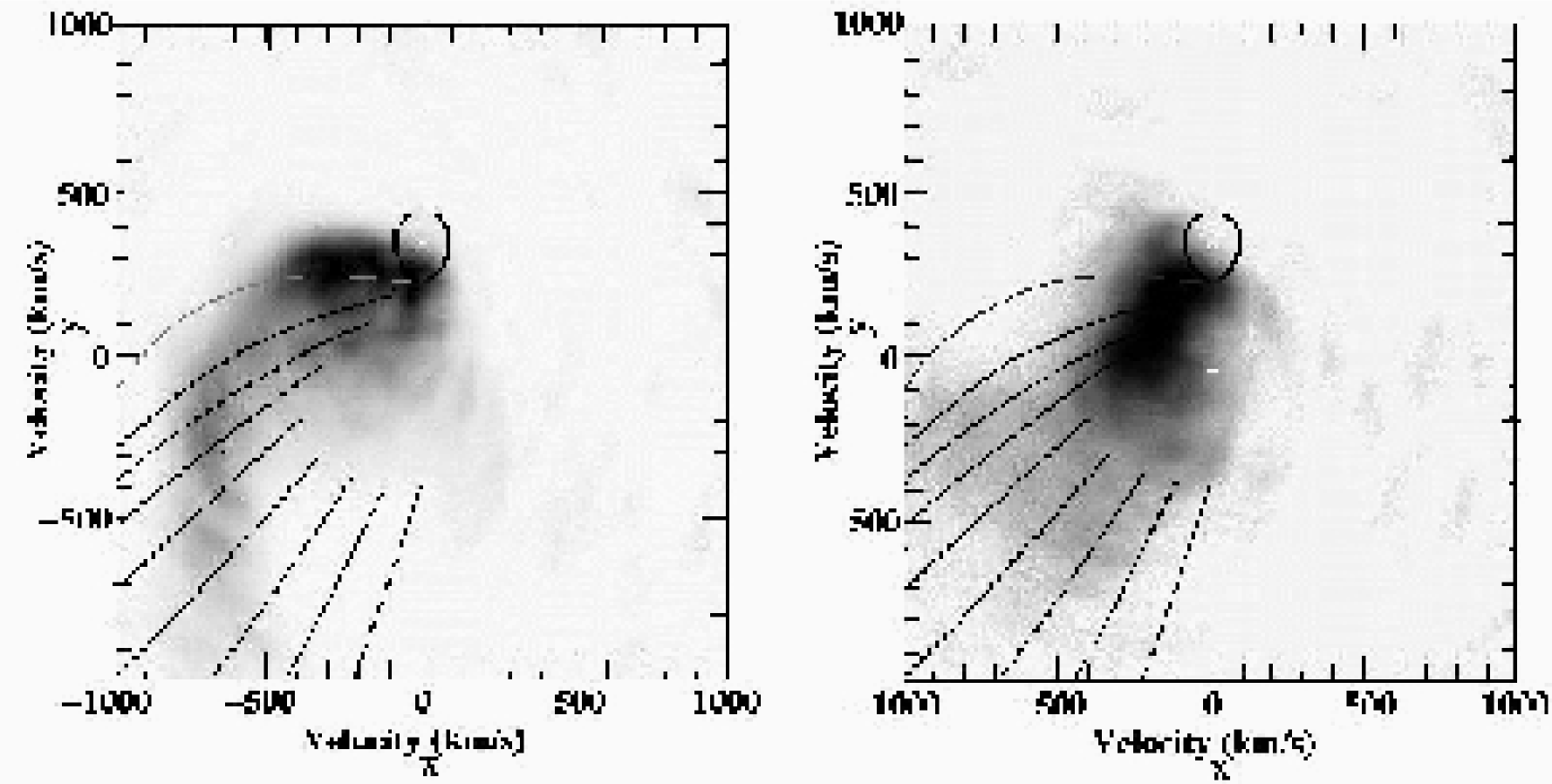
It is now possible to discern four and possibly five emission components. From Fig. 4e we can see emission at the expected location of the secondary star v, v km s-1, the ballistic stream (the ridge of brightness starting at v km s-1 and extending from v km s-1 to v km s-1) and emission at a location that may be consistent with part of the magnetic stream (region of emission centered on v -300, v km s-1). In addition, Fig. 4j shows a fourth component, consistent with the part of the magnetic stream that has just left the orbital plane (the diagonal region extending from v, v km s-1 to v, v km s-1. Furthermore, there is a fainter but broad emission feature that occupies most of the lower left-hand quadrant of the Doppler tomogram, which can be seen more clearly in the right plot of Fig. 5. Therefore, in what follows, we will use the tomograms of Fig. 4e and 4j, which have been reproduced in Fig. 5, in order to model and interpret the dynamical components of the binary system.
3.2.1 Single particle trajectory
Our next step is to model the ballistic and magnetic streams of the tomograms in order to gain a quantitative understanding of their trajectories and to locate the footprints of the magnetic field lines on the surface of the white dwarf. We can then compare the location of the magnetic field lines with the location of the cyclotron emission region predicted from Stokes imaging.
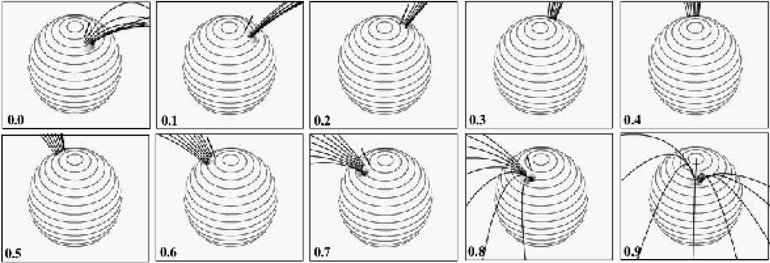
On the tomograms of Fig. 5 (reproduced from Figs. 4e and 4j) we have overplotted a model trajectory computed using a single particle under gravitational and rotational influences, shown as the upper curved lines. No additional drag terms (e.g. due to the magnetic field) are included. The particle is allowed to follow a ballistic path from the L1 point and is terminated 75 degrees in azimuth around the white dwarf. At 10 degree intervals in azimuth (from 5 to 75 degrees) around the white dwarf, dipole trajectories are calculated (the straighter diagonal lines below the ballistic trajectory) from the ballistic stream to the surface of the white dwarf. The first dipole trajectory starts close to the location of the secondary star, with the consecutive trajectories starting at locations progressively closer to the white dwarf. The velocity of the particle in the direction of the field is conserved when it attaches onto a field line. At the threading region, the re-direction of the particle is quite large in Doppler velocity space, hence the beginning of the magnetic streams appear disjointed from the ballistic stream.
The Doppler velocities are dependent on the inclination of the binary system, the magnetic dipole angles and the mass ratio of the binary. We used the same values as those for Stokes imaging, namely an inclination of 50 degrees and dipole offset angles (latitude and longitude) of 20 and 36 degrees respectively, consistent with those calculated by Ferrario et al. (1992) and Schwope et al. (1993). The magnetic dipole was again offset by -0.1 white dwarf radii along the dipole axis, consistent with the findings of Ferrario et al. (1992). A mass ratio and white dwarf mass of 0.85M☉ were used, consistent (within the errors) with Schwope et al. 1993, () but somewhat higher than estimates from X-ray observations (Ramsay 2000, ). The center of mass of the secondary star and the primary star are indicated by a ‘+’ and a ‘*’ respectively. Also indicated is the Roche lobe of the secondary star.
With this geometry, the single particle ballistic stream traces the lower part of the emission fairly well (left panel Fig. 5). Interestingly, the observed ballistic stream does not appear to be dislocated to lower Doppler velocities as observed in other systems. This is discussed later in the discussion section. The model ballistic trajectory is calculated up to more than 40 degrees further than the end of the ballistic emission seen in the tomogram.
The diagonal region extending from v, v km s-1 to v, v km s-1 (Fig. 5 right plot) corresponds to the low Doppler velocities of the threading region, from which most the calculated magnetic trajectories point to.
The dipole trajectories also overlap with the emission seen centered on v -700 km s-1 and v -300 km s-1 (best seen in the left plot of Fig. 5). According to the calculated dipole trajectories, this area corresponds to the highest point above the orbital plane where the dipole trajectory “turns over”, but see section 4.1.
The broad fainter emission, seen in the lower left quadrant of the Doppler tomograms (best seen in the right plot of Fig. 5), appears to correspond to the full range of calculated dipole trajectories (5-75 degrees), suggesting that threading of the magnetic field lines occurs from a ballistic stream that extends by more than 40 degrees further than the Doppler ballistic emission suggests.
However, it should be noted that the inclination of V834 Cen is thought not to be very high, thus the out of plane velocities of the dipole trajectory would lead to a smearing effect of the corresponding emission in the Doppler tomograms. Thus a more detailed modelling than presented here could lead to over interpretation.
3.3 Roche tomography
Roche tomography (Rutten & Dhillon 1994; Watson & Dhillon 2001; Dhillon & Watson 2001) is a technique used for imaging the Roche-lobe-filling secondary stars in CVs. The secondary star is modelled as a series of quadrilateral surface elements. Each element is assigned its own local intrinsic specific intensity profile, which are scaled to take into account the projected area, limb darkening and obscuration. Every element is then Doppler shifted to the radial velocity of the surface element at that particular phase. All the elements are then summed to give the rotationally broadened profile at any particular orbital phase. By iteratively varying the strengths of the profile contributed from each element, the ‘inverse’ of the above procedure can be performed and thus Roche tomograms present images of the distribution of line flux on the secondary star.
Due to the variable and unknown contribution to the spectrum of the accretion region in V834 Cen, the data should ideally be slit-loss corrected and continuum subtracted. The observations of V834 Cen have not been slit-loss corrected, but we have folded the observations, which cover several orbits, into twenty phase bins on the orbital period, thus smearing out any effects due to random slit losses. In addition we note that the transparency and seeing conditions were excellent during all the observing runs and the slit-losses are thought to be minimal. The data have been continuum subtracted.
We next fit Gaussians to the HeII 4686 Å emission line profile in each of the phase bins. During fitting, the solution from the previous bin was used as a starting point for each consecutive bin. From these fits we then extracted the parameters of the Gaussian that describes the narrow component of the HeII emission line, which is thought to arise from the irradiated face of the secondary. We then selected data from only those phases where the narrow component is clearly distinguishable from the other components. This is necessary in order to minimise any artifacts that will arise in the Roche map as a result of contamination of the input data from other components in the binary system (e.g. from the accretion stream).
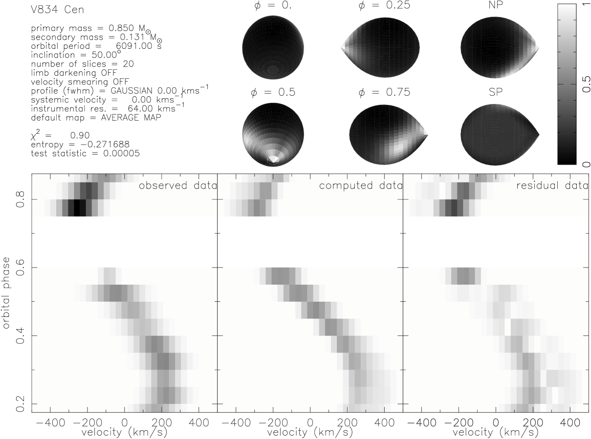
The Roche tomogram of V834 Cen obtained from the HeII 4686 Å emission line is presented in Fig. 6. Also shown are the input data and the computed data. There are two prominent asymmetries evident in the tomograms. Firstly, a comparison of the Roche surface presented at phases 0.25 and 0.75 reveals the leading face of the secondary to be brighter than the trailing face. Secondly, the view of the Roche surface from its north pole reveals that the inner surface (the face of the secondary most pointing towards the white dwarf) is brighter than the outer surface. These asymmetries can be explained as a result of irradiation. This is discussed further in section 4.
4 Discussion
4.1 The system parameters
As explained above, the calculated Doppler trajectory of the ballistic stream depends on the system parameters, namely the inclination and the mass ratio of the binary. We show in Fig. 7 the results of calculating ballistic trajectories for a range of system parameters and comparing them to the observed ballistic emission seen in the tomograms. The thicker, upper solid curve of Fig. 7 represents the range of system parameters that produce ballistic streams which trace the center of the observed ballistic Doppler emission fairly well. The lower and upper dashed curves define system parameters that give ballistic trajectories that lie just below and above the observed ballistic emission respectively.
The lower four curves of Fig. 7 are reproduced from figure 5 of Schwope et al. (1993) and show their predictions for the system parameters of V834 Cen based on modelling the velocities of the secondary. More details of their model can be found in Beuermann & Thomas (1990). The dotted curves represent different estimates of .
From Fig. 7, it is therefore immediately obvious that the ballistic trajectories generally predict higher inclinations and/or mass ratios than modelling. This is wholy unexpected, as previous investigations of other systems such as HU Aqr (Schwope et al. 1997, Heerlein et al. 1999) and QQ Vul (Schwope et al. 2000) have shown the opposite to be true (see also the discussion by Schwope 2001). The main reason for previous findings was thought to be that the, so-called, ballistic trajectory is not purely ballistic, but suffers from a magnetic influence. This may either introduce a magnetic drag to the ballistic particles and therefore slow them down (see Sohl & Wynn 1999), or the magnetic field is perhaps diverting the stream to lower Doppler velocities. Our V834 Cen stream appears to be more ballistic and/or less affected by magnetic influences.
The overlap between the two models is minimal, with the center of the overlap region being located at an inclination of 50 degrees with a mass ratio of 6.5, giving a white dwarf mass of 0.85M☉. The fit obtained with Roche tomography, using the adopted parameters, (i.e. an inclination of 50 degrees and a mass ratio of 6.5) predicts slightly higher velocities than observed. Therefore Roche tomography prefers lower inclinations and/or mass ratios which are, not surprisingly, more inline with the velocity work of Schwope et al. (1993). Stokes imaging is independent of mass ratio, but it does predict a best inclination of 50 degrees (although the larger range of 45-60 degrees cannot be excluded).
A mass ratio of 6.5 is relatively large amongst the magnetic Cataclysmic Variables, and perhaps a possible reason for a true ballistic stream. The high mass ratio may be enough to give the ballistic stream sufficient ram pressure to overcome the magnetic field of the white dwarf for at least some distance. We also point out that our observations were taken when V834 Cen was in a high state, implying a higher accretion rate and thus the ballistic stream would have even more ram pressure than usual. Once the ballistic stream has become sufficiently close to the white dwarf, its magnetic field begins to dominate the flow of the stream, and the remaining ballistic stream may even disappear from the Doppler tomogram as the velocities become smeared. Another possibility may be that the magnetic field geometry is such that its influence over the ballistic stream is not very strong at the beginning of the ballistic trajectory.
In section 3.2 we briefly mentioned that the bright emission region centered on v -300, v km s-1 may correspond to the highest point above the orbital plane where the dipole trajectory “turns over”. It may, however, be of ballistic origin rather than magnetic origin. From the range of system parameters defined by the models in Fig. 7, it is not possible to ’make’ the simple, single particle ballistic stream go through this region. However, we expect that adding an arbitrary amount of magnetic drag could deflect the ballistic trajectory through this region. Support for a ballistic stream that continues further than the Doppler map suggests can further be obtained from EUVE (Extreme UltraViolet Explorer) observations (Mauche 2002). That analysis placed the EUV emission at a location on the white dwarf, approximately 40 degrees in azimuth, extending to over 70 degrees when V834 Cen is observed in a high state.
4.2 The accretion region
As mentioned in section 3.1, Fig. 2 shows the white dwarf of V834 Cen for a complete orbital rotation, as viewed from Earth. In this spatial coordinate frame we have also plotted the magnetic field lines that were derived from the modelling of the Doppler tomograms (section 3.2). Upon close examination it is clear that footprints of the magnetic field lines on the surface of the white dwarf coincide fairly well with the location of the cyclotron emission region predicted from Stokes imaging. In addition, the general longitudinal extent of the cyclotron emission runs along the footprints of the magnetic field lines. Furthermore, the brightest part of the cyclotron emission region coincides with the magnetic field lines connecting with the end of the ballistic stream, thus adding further support that magnetic accretion does occur towards the end of the ballistic stream.
As already mentioned above, the EUV emission emanates from a similar location on the surface of the white dwarf (see Mauche 2002).
4.3 Irradiation of the secondary
The Roche tomogram displayed in Fig. 6 shows that the HeII emission distribution to be stronger on the leading face of the secondary star. A close inspection of the tomograms in Figs. 4b-d also indicate a possible asymmetry towards the leading face of the secondary. This is contrary to other magnetic Cataclysmic Variables for which HeII Roche tomography is available.
It is generally accepted that the HeII emission from the Roche surface of the secondary is as a result of irradiation by the accretion shock. Watson et al. (2003) found for three magnetic CVs (AM Her, QQ Vul and HU Aqr), that the irradiation pattern (from HeII emission and Na I absorption roche tomograms) was mostly on the trailing faces of the secondary stars. They reasoned that the accretion stream/column was somehow shielding the leading face of the secondary from the shock on the surface of the white dwarf.
In the case of V834 Cen we must, therefore, reason that any shielding is somehow minimal. Instead, the leading face of the secondary is more irradiated because of the simple reason that, from its position within the orbital frame, it has a better ’view’ of the accretion shock. This is particularly true for V834 Cen because, as we have shown in section 3, the accretion shock points ahead in orbital phase. In addition, the Doppler maps show quite clearly that the inner part of the ballistic stream is a dominant source of HeII line emission. This too will irradiate the leading face of the secondary, but not the trailing face because this side will be shielded by the secondary itself. Furthermore, as we have already discussed, the earlier parts of the ballistic stream do not appear to be magnetically influenced, hence the accretion curtain, if present, probably does not form until further down the stream and is therefore less likely to act as a shield of the irradiating source.
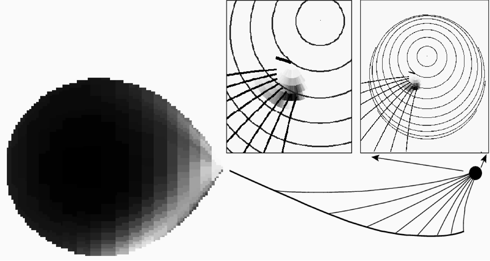
This is illustrated in Fig. 8, which shows a schematic view from above the orbital plane of our derived geometry for V834 Cen. The eight magnetic field lines correspond to the same magnetic field lines drawn in the earlier Doppler maps. From the insert one can see that most of the cyclotron emission comes from near the footprints of the magnetic field lines that originated from the latter parts of the ballistic stream. If indeed the denser parts of the accretion curtain are located on these magnetic field lines, then from Fig. 8 one can see that they will not shield the secondary from the white dwarf.
5 Summary and Conclusions
We have presented new photopolarimetric and spectroscopic observation of the AM Herculis binary V834 Cen during a high state of accretion. The observed high levels of polarization over the whole orbit are modelled using Stokes imaging. This technique predicts a single emission region, visible for the whole orbit, to be responsible for the observed polarized variations. The location of the region on the white dwarf is consistent with recent work on EUV observations by Mauche (2002). Both analyses place the main emission region approximately more than 40 degrees and up to 70 degrees in azimuth from the line of centers of the two stars.
Our Doppler tomographic analysis shows several components associated with the secondary star, the ballistic stream and parts of the magnetically confined stream. Interestingly, the ballistic stream (at least the earlier parts) do not show a reduced Doppler velocity as is commonly seen in other polars. We therefore reason that the earlier part of the ballistic stream is relatively free from magnetic influences of the white dwarf. Magnetic Doppler trajectories are also calculated and shown to be generally coincident with the magnetic signatures found in the Doppler maps. We also calculated the location of the footprints of the magnetic field lines on the surface of the white dwarf and showed that these are coincident with the prediction for the location of the cyclotron emission region from Stokes imaging.
Roche tomography of the narrow component seen in the HeII 4686 Å emission line reveals two asymmetries in the emission distribution on the Roche surface of the secondary. Namely, there is generally more emission on the inner surface and also on the leading face of the secondary. We argue that this is still consistent with irradiation of the secondary, as the lack of a magnetic curtain at the beginning of the ballistic stream reduces its obscuring ability. This is not only supported by the Doppler tomogram, but also by Stokes imaging results, which show that most of the accreting material comes along field lines that intersect the later parts of the ballistic stream (see Fig. 8).
6 Acknowledgments
CAW is employed on PPARC grant PPA/G/S/2000/00598.
References
- [1] Bailey J., Axon D. J., Hough J. H., Watts D. J., Giles A. B. & Greenhill J. G., 1983, MNRAS, 205, 1p
- [2] Beuermann K. & Thomas H.-C, 1990, A&A, 230, 326
- [3] Charbonneau P., 1995, ApJS, 101, 309
- [4] Cropper M. S., 1985, MNRAS, 212, 709
- [5] Cropper M. S., Menzies J. W. & Tapia S., 1986, MNRAS, 218, 201
- [6] Cropper M. S., 1990, Space Sci. Rev. 54,195
- [7] Cropper M. S., 1997, MNRAS, 289, 21
- [8] Dhillon V. S., & Watson C. A., 2001, in Boffin H., Steeghs D., eds, Lecture Notes in Physics, Astrotomography, Indirect Imaging Methods in Observational Astronomy, Springer-Verlag, Berlin, p. 94
- [9] Ferrario L. & Wickramasinghe D. T., Bailey J., Hough J. H. & Tuohy I. R., 1992, 256, 252
- [10] Heerlein C., Horne K. & Schwope A. D., 1999, MNRAS, 304, 145
- [11] Hsu J. C. & Breger M., 1982, ApJ, 262, 732
- [12] Jensen K. A., Nousek J. A. & Nugent J. J., 1982, ApJ, 261, 625
- [13] Mason K. O., et al., 1983, MNRAS, 264, 575
- [14] Marsh T. R. & Horne K., 1988, MNRAS, 235, 269
- [15] Marsh T., 2001 , in Boffin H., Steeghs D., eds, Lecture Notes in Physics, Astrotomography, Indirect Imaging Methods in Observational Astronomy, Springer-Verlag, Berlin, p. 1
- [16] Mauche C. W., 2002, ApJ, 578, 439
- [17] Potter S. B., Hakala P. J. & Cropper Mark, 1998, MNRAS, 297, 1261
- [18] Potter et al. 2001 in Boffin H., Steeghs D., eds, Lecture Notes in Physics, Astrotomography, Indirect Imaging Methods in Observational Astronomy, Springer-Verlag, Berlin, p. 244
- [19] Potter S. B., Ramsay G., Wu K. & Cropper M., 2002 in Gänsicke B. T., Beuermann K. & Reinsch K., eds, ASP Conf. Ser. Vol. 262, The Physics of Cataclysmic Variables and Related Objects, p. 165
- [20] Puchnarewicz, E. M., Mason K. O., Murdin P. G., & Wickramasinghe D. T., 1990, MNRAS, 244, 20p
- [21] Ramsay G., 2000, MNRAS, 314, 403
- [22] Rosen, S. R., Mason K. O. & Còrdova F. A., 1987, MNRAS, 224, 987
- [23] Rutten R. G. M. & Dhillon V. S., 1994, A&A, 288, 773
- [24] Schwope A. D. & Beuermann K., 1990, A&A, 238, 173
- [25] Schwope A. D., Thomas H.-C., Beuermann K. & Reinsch K., 1993, A&A, 267, 103
- [26] Schwope A. D., Mantel K.-H. & Horne K., 1997, A&A, 319, 894
- [27] Schwope A. D., Catalán M. S., Beuermann K., Metzner A., Smith R. C. & Steeghs D., 2000, MNRAS, 313, 533
- [28] Schwope A. D. 2001, in Boffin H., Steeghs D., eds, Lecture Notes in Physics, Astrotomography, Indirect Imaging Methods in Observational Astronomy, Springer-Verlag, Berlin, p. 127
- [29] Sohl K. B. & Wynn G., 1999, ASP Conf. Ser., 157, 87
- [30] Spruit H. C., 1998, preprint (astro-ph/9806141)
- [31] Tapia S., 1982, IAU Circ. No. 3685
- [32] Warner B. 1995, Cataclysmic Variable Stars, Cambridge Astrophysics Series 28, Cambridge University Press
- [33] Watson C. A. & Dhillon V. S., 2001, MNRAS, 326, 67
- [34] Watson C. A., Dhillon V. S., Rutten R. G. M. & Schwope A. D., 2003, MNRAS, 341, 129
- [35] Wickramasinghe D. T. & Meggitt S. M. A., 1985, MNRAS, 214, 605
- [36] Wickramasinghe D. T., Tuohy I. R. & Visvanathan N., 1987, ApJ, 318, 326