Simulation of Soft X-ray Emission Lines from the Missing Baryons

Abstract

We study the soft X-ray emission (0.1 – 1 keV) from the Warm-Hot Intergalactic Medium (WHIM) in a hydrodynamic simulation of a Cold Dark Matter universe. Our main goal is to investigate how such emission can be explored with a combination of imaging and spectroscopy, and to motivate future X-ray missions. We first present high resolution images of the X-ray emission in several energy bands, in which emission from different ion species dominates. We pick three different areas to study the high resolution spectra of X-rays from the warm-hot IGM: (a) a galaxy group; (b) a filament and (c) an underluminous region. By taking into account the background X-ray emission from AGNs and foreground emission from the Galaxy, we compute composite X-ray spectra of the selected regions. We briefly investigate angular clustering of the soft-X-ray emission, finding a strong signal. Most interestingly, the combination of high spectral resolution and angular information allows us to map the emission from the WHIM in 3 dimensions. We cross-correlate the positions of galaxies in the simulation with this redshift map of emission and detect the presence of six different ion species (Ne IX, Fe XVII, O VII, O VIII, N VII, C VI) in the large-scale structure traced by the galaxies. Finally we show how such emission can be detected and studied with future X-ray satellites, with particular attention to a proposed mission, the Missing Baryon Explorer, or $\sl MBE$. We present simulated observations of the WHIM gas with $\sl MBE$.

1. Introduction

Cosmological hydrodynamic simulations provide us with quantitative predictions for the state of baryonic matter in the universe (see, e.g, Cen & Ostriker, 1999; Davé et al., 2001). At high redshift ($z\gtrsim 3$), most baryons are diffuse, with a density close to the cosmic mean, and are located in the intergalactic medium (IGM). They can be probed readily using Ly$\alpha$ absorption systems in the optical spectra of high redshift quasars (see e.g., Cen et al., 1994; Zhang, Anninos, & Norman, 1995; Hernquist, Katz, Weinberg, & Jordi, 1996; Weinberg et al., 1997). At low redshift, the process of gravitational collapse has caused a minority of baryons to condense into structures such as stars, galaxies, groups and clusters of galaxies. While a substantial fraction ($\sim$ 30%) of baryons are trapped within the gravitational potential wells of these large scale structures in the form of hot intracluster or intragroup gas, the remaining baryons are left in intergalactic space and are predicted to form filamentary structures seen in cosmological hydrodynamic simulations. Some of these structures contain baryons with relatively low temperatures ($T\lesssim 10^{4}$ K), and therefore enough residual neutral hydrogen to be detectable as the low-redshift Ly$\alpha$ forest (see, e.g., Davé, Hernquist, Katz, & Weinberg, 1999; Penton, Shull, & Stocke, 2000). However, a larger fraction have been shock-heated to temperatures between $10^{5}-10^{7}$ K. Given these temperatures, these baryons, which form the so-called “warm-hot intergalactic medium,” or “WHIM,” are best probed using UV/X-ray observations.

Recently, important progress has been made in the detection of absorption features produced by highly ionized metals in this WHIM gas in the UV/X-ray spectra of background quasars. In the UV band, a significant number of O VI absorption lines have been seen with the Far Ultraviolet Spectroscopic Explorer ($\sl FUSE$) and the Hubble Space Telescope ($\sl HST$) (see, e.g., Savage, Tripp, & Lu, 1998; Tripp, Savage, & Jenkins, 2000; Tripp & Savage, 2000; Simcoe, Sargent, & Rauch, 2002). The distribution and derived properties of these O VI lines are consistent with predictions from simulations (see, e.g., Fang & Bryan, 2001; Cen, Tripp, Ostriker, & Jenkins, 2001; Chen, Weinberg, Katz, & Davé, 2003). In the X-ray band, Fang et al. (2002), Mathur, Weinberg, & Chen (2002), Cagnoni (2002) and McKernan et al. (2003) reported on the detection of intervening O VII and/or O VIII absorption lines with Chandra and XMM-Newton. Nicastro et al. (2002), Fang, Sembach, & Canizares (2003) and Rasmussen, Kahn, & Paerels (2003) also reported the detection of $z\approx 0$ X-ray absorption lines. These low redshift lines may be attributable, at least in part, to the WHIM gas in our Local Group.

The absorption line method does have the advantage of directly probing the absorbing ions, as the detected line strength is proportional to the column density and so to the ion number density. However, it suffers the limitation of being only able to probe one dimensional information, along limited lines of sight, and detectability is also constrained by the flux of background sources. In order to fully reveal the three dimensional structure and physical properties of the WHIM gas, we need to study its emission with imaging/spectroscopic methods. In this paper, we will focus on the X-ray emission from the WHIM gas. In general, X-ray emission from a hot, diffuse plasma contains two parts, a continuum which is contributed by various emission mechanisms, and line emission from metals in the IGM. While we will briefly discuss the continuum emission from the WHIM, this paper will be devoted mostly to studying the line emission.

Several authors have extensively studied the broad band soft X-ray emission (0.5 – 2 keV) from the diffuse background, particularly the X-ray emission from the WHIM gas, using hydrodynamical simulations (see, e.g., Cen, Kang, Ostriker, & Ryu, 1995; Phillips, Ostriker, & Cen, 2001; Croft et al., 2001). Much effort has been put into investigating the overall intensity of the emission, and how to distinguish it from the two dominant sources of the soft X-ray background: X-ray emission from active galactic nuclei (AGNs) and from the hot gas in our Galaxy (see, e.g, Kuntz & Snowden, 2000; Kuntz, Snowden, & Mushotzky, 2001). Simulations predict that the mean intensity of emission from the WHIM gas is between (2 – 4) $\times 10^{-13}\rm\ ergs\ s^{-1}cm^{-2}deg^{-2}$, only about 5 – 15% of the total extragalactic X-ray emission between 0.5 – 2 keV (Phillips, Ostriker, & Cen, 2001; Croft et al., 2001). While it seems to be a difficult task to detect most of this WHIM emission with current X-ray telescopes, it appears feasible to detect the high intensity tail of the WHIM X-ray intensity distribution. For instance, Scharf et al. (2000) reported on the presence of a possible filament with intensity $\approx 6\times 10^{-13}\rm\ ergs\ s^{-1}cm^{-2}deg^{-2}$ with the ROSAT PSPC; and Markevitch et al. (2003) and Kaastra et al. (2003) reported detecting O VII and/or O VIII from an extended, diffuse structure, possibly from WHIM gas; and McCammon et al. (2002) recently performed a large-field ($\sim$ 1 sr), high spectral resolution (5 – 12 eV) observation with a sounding rocket and detected C V/O VII/O VIII lines from the diffuse background, some fraction of which may be from the WHIM at zero redshift.

We expect that future X-ray missions will enable high resolution imaging/spectroscopic observations of the emission from the WHIM gas. We explore such a scenario with a high resolution hydrodynamic simulation in this paper. Our purpose is to address two important questions: with high spectral/spatial resolution, what does the X-ray emission from the diffuse, hot gas in intergalactic space look like; and are proposed future X-ray missions capable of conducting useful observations? Particularly, we will focus on a proposed mission called the Missing Baryon Explorer, or $\sl MBE$. Given its large field-of-view ($29.5\arcmin\times 29.5\arcmin$), high spectral ($\sim 4$ eV) and moderate angular ($\sim 5\arcmin\times 5\arcmin$) resolution, we find that $\sl MBE$ will be capable of revealing the X-ray emission from the WHIM gas. In addition, we will explore the clustering properties of the WHIM gas, and its correlation with nearby large scale structures traced by galaxies.

Recently, Yoshikawa et al. (2003) examined the detectability of the X-ray emission from the WHIM gas independently with a similar numerical approach. They presented a detailed study of O VII and O VIII emission lines from WHIM. They also investigated a dedicated X-ray mission, DIOS (Diffuse Intergalactic Oxygen Surveyor). It turns out that DIOS and MBE very similar properties. While there are some differences between our work and theirs, such as the selection of the energy bands (Yoshikawa et al., 2003 concentrated on 0.5 – 0.7 keV while we look at a broader band between 0.1 – 1 keV) and the choice of the IGM metallicity models, where they can be compared our results agree with each other reasonably well.

Our plan for this paper is as follows. We give a brief explanation of the simulation method and our treatment of the simulation data in §2. A full study of the emission from the WHIM gas is presented in §3, followed by measurement of its auto- and cross-correlation properties, making use of the galaxy distribution in the simulation for the latter. We investigate the detectability of emission with the proposed MBE X-ray telescope in §5, and §6 is our discussion and summary.

2. Simulation

We use a cosmological hydrodynamic simulation studied by Davé et al. (2001) (their model D1). It was run with PTreeSPH, or parallel tree smoothed particle hydrodynamics (see Davé, Dubinski, & Hernquist, 1997). We refer the reader to these two papers as well as Croft et al. (2001) for more details. The model simulated is a Cold Dark Matter (CDM) universe with a cosmological constant ($\Lambda$CDM), with cosmological parameters $\Omega_{\Lambda}=0.6$ and $\Omega_{m}=0.4$. The parameter $h=0.65$, where the Hubble constant is $H_{0}=100h\rm\ km\ s^{-1}Mpc^{-1}$. The simulation box size is $50h^{-1}\rm Mpc$ with a $7h^{-1}\rm kpc$ spatial resolution (comoving units, equivalent Plummer softening). The baryonic mass resolution is $8.5\times 10^{8}\ M_{\odot}$, where $M_{\odot}$ is the solar mass. Cooling from H and He was included, as well as star formation and mild feedback. As discussed in Davé et al. (2001), the feedback consists of thermal energy which is released into star forming regions, which are of high density. The energy is rapidly radiated away and has little effect on the IGM. The simulation was run from redshift $z=49$ to the present. We make use of 27 of the outputs, roughly logarithmically spaced in redshift,ranging from $z=5.98$ to $z=0$.

For each gas particle, we calculate the X-ray emissivity based on a Raymond-Smith code (Raymond & Smith, 1977). Note that we have first recalculated the SPH densities for each X-ray emitting particle after excluding the cold particles from the density estimator (see Croft et al., 2001 for details). This decoupling of hot and cold phases (see also Pearce et al., 2000, for example) is necessary in order avoid overestimating the densities of hot particles which are close to cold particles (see also Springel & Hernquist, 2002).

We adopt a density-dependent metallicity, $Z\propto\sqrt{\rho/\overline{\rho}}$, to mimic the density-metallicity relation obtained by Cen & Ostriker (1999), Springel & Hernquist (2003), and Aguirre et al. (2001a,b,c) in their simulations. Here $\rho$ and $\overline{\rho}$ are the density and the mean density of the universe. We normalize this relation by setting $Z=0.005Z_{\odot}$ at $\rho=\overline{\rho}$ to match Ly$\alpha$ forest measurements, and limiting the metallicity to be $Z\leq 0.3Z_{\odot}$ in much more overdense regions to match the observational results from galaxy clusters in the local universe. Here $Z_{\odot}$ is the solar abundance. The Raymond-Smith code includes eleven heavy elements, namely C, N, O, Ne, Mg, Si, S, Ar, Ca, Fe, and Ni. Table 1 lists the wavelengths and the corresponding energies of the strongest emission lines we are probing with our simulation. Assuming collisional ionization equilibrium, Figure 1 shows the emissivity $\epsilon_{i}$ for each ion species (Raymond & Smith, 1977), where $i$ represents ion species $X_{i}$. We give the strongest line (the resonance line in the He-like triplet), and for Fe XVII we select the 825.79 eV line.

In Figure 2 we display three template X-ray emission spectra for hot gas at different temperatures: (a) T = $10^{6}$ K; (b) T = $10^{6.5}$ K; (c) T = $10^{7}$ K. We use a metallicity of 0.1 $Z_{\odot}$, which is typical for gas with overdensities $\delta\sim$ a few hundred based on simulations (Cen & Ostriker (1999), Springel & Hernquist (2003)). Here $\delta$ is defined as $\delta\equiv\rho/\overline{\rho}-1$. Figure 2a and  2b show that at low temperatures the spectra are dominated by C, N and O VII emission lines. At high temperatures O VIII and Fe emission start to take over. At temperatures above $10^{7}$ K, the spectra are completely dominated by Fe and Ne emission lines.

Table 1: Emission Line List
Ion	Wavelength ($\AA$)	Energy (eV)	$\rm Line^{1}$	$\rm Reference^{2}$
C V	41.47	298.96	f	a
	40.73	304.41	i	a
	40.27	307.89	r	a
C VI	33.73	367.54		b
N VI	29.53	419.79	f	a
	29.08	426.30	i	a
	28.78	430.80	r	a
N VII	24.78	500.35		b
O VII	22.10	560.98	f	a
	21.80	568.62	i	a
	21.60	573.95	r	a
O VIII	18.97	654.00		b
Fe XVII	17.10	725.22		c
	17.05	727.14		c
	16.78	738.88		c
	15.01	825.79		c
Ne IX	13.70	905.10	f	a
	13.55	915.03	i	a
	13.45	922.00	r	a

1. Line: r — resonance; i — intercombination; f — forbidden
2. Reference: a. Drake (1988); b. Johnson & Soff (1985); c. Brown et al. (1998)

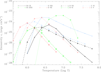
Figure 1.— X-ray emissivity for eight ion species. Among them, O VII, O VIII, and Fe XVII show the highest peak emissivities between $10^{6}$ – $10^{7}$ K. Emission models were taken from Raymond & Smith (1977).

Figure 2.— X-ray emissivity for hot gas at three temperatures typical of the $z=0$ IGM: (a) T = $10^{6}$ K; (b) T = $10^{6.5}$ K; (c) T = $10^{7}$ K. The gas has a metallicity of 0.1 $Z_{\odot}$. Emission models were taken from Raymond & Smith (1977).

Three types of continuum emission make contributions to the total X-ray continuum we discuss here: thermal bremsstrahlung radiation, or free-free emission; radiative recombination radiation, or free-bound emission; and two-photon decay (see. e.g., Raymond & Smith, 1977). Their relative contributions vary with temperature and photon energy. For instance, at T $\sim 10^{6}$ K radiative recombination dominates at E $>0.4$ keV, while thermal bremsstrahlung radiation dominates over the entire X-ray band when T $\sim 10^{7}$ K. The total continuum emissivity $\epsilon_{c}$, as a function of photon energy $E$, can be written as (Mewe & Gronenschild, 1981):

$$\epsilon_{c}(E)\propto\overline{G_{c}}(E,T)ET^{-1/2}n^{2}_{e}\exp(-E/kT),$$ (1)

where $T$ is the gas temperature, $n_{e}$ is the electron density, $k$ is Boltzmann’s constant, and $\overline{G_{c}}(E,T)$ is the total effective Gaunt factor, which includes all three continuum emission processes (Gronenschild & Mewe, 1978). By integrating $\epsilon_{c}(E)$ over energy $E$, the integrated X-ray continuum emissivity is $\propto n^{2}_{e}T^{\alpha}$, where $\alpha=1/2$ for high temperature gas, in which bremsstrahlung radiation dominates, and $\alpha=-3/2$ for gas with $T\lesssim$ a few $\times 10^{6}$ K.

3. Soft X-ray Spectra of the Warm-Hot Intergalactic Medium

3.1. The IGM: simulated maps and spectra

In order to go from the three dimensional particle distributions in the simulation outputs to sky maps and spectra, we rely on the technique of stacking simulation boxes along the lightcone (see e.g., da Silva et al., 2000; Springel, White, & Hernquist, 2001; Croft et al., 2001). We place simulation boxes one behind the other until we reach the comoving distance corresponding to a given redshift ($z=1$ in the first case). The output file corresponding to the closest redshift is used at each point (we use 11 different outputs between $z=0$ and $z=1$). The boxes are randomly rotated, reflected and translated (Croft et al., 2001) so that periodic structure does not repeat along the line of sight. Because of this, only structure on scales smaller than the box is preserved, and we only consider structure on these scales when measuring clustering statistics. For example, the median redshift of emission is $z=0.45$ in the $0.5-2$ keV band, so that we cannot accurately simulate structure with angular scales $\gtrsim$ 100 arcmins.

The X-ray emissivity in a range of 2eV wide bins in energy is computed for each particle, and these quantities are allocated to a grid using the projection of the SPH kernel on the plane of the sky (see below for more details). The grid is a three dimensional datacube, with two angular axes and one axis for photon energy.

We first examine the angular distribution of the emission in a relatively broad spectral band. In Figure 3 we show a map of a $200\arcmin\times 200\arcmin$ simulated region. The area has been divided into a 512$\times$512 grid, so that each pixel has side length $\sim 23\arcsec$. The X-ray emission includes both continuum and metal line emission from the hot IGM, integrated between 0.1 – 1 keV. Croft et al. (2001) showed that the majority of the X-ray emission from the IGM received at $z=0$ comes from gas with $z<1.0$ (about 90%, see Figure 11a of Croft et al., 2001). Due to dilution by projection, filaments that would be apparent in three dimensions do not appear readily here. The intensity varies from $10^{-6}-10^{-7}\rm\ erg\ s^{-1}cm^{-2}deg^{-2}$, in patches of sky dominated by emission from the hot IGM in groups or clusters of galaxies, down to $10^{-14}\rm\ erg\ s^{-1}cm^{-2}deg^{-2}$, in regions of low density. We label three ($5\arcmin\times 5\arcmin$) areas that we will study in detail spectroscopically in the following sections: area (a), with an average surface brightness of $10^{-7}\rm\ erg\ s^{-1}cm^{-2}deg^{-2}$, representing X-ray emission from a galaxy group; area (b), with a mean surface brightness of $10^{-9}\rm\ erg\ s^{-1}cm^{-2}deg^{-2}$, representing X-ray emission from a superposition of filamentary structures; and area (c), with a surface brightness of $10^{-13}\rm\ erg\ s^{-1}cm^{-2}deg^{-2}$, an underdense and void-like region.

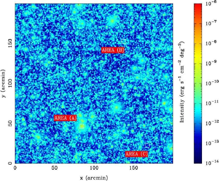
Figure 3.— The simulated $200\arcmin\times 200\arcmin$ region. The whole region is divided into 512$\times$512 grid cells, and the X-ray intensity is each cell is obtained by integrating the X-ray flux between 0.1 – 1 keV in that cell. We select three regions (shown as white boxes) to study three typical types of X-ray emission: (a) hot gas in a galaxy group; (b) diffuse X-ray emission in a filament; and (c) a void.

Figure 4 shows the soft X-ray emission from the same sky area but in four narrower energy bands. Since the X-ray continuum emissivity exponentially decreases with energy, in most energy intervals the flux from the X-ray emission lines dominates over the continuum emission. In panel (a) emission lines from carbon, particularly C VI and C V triplet dominate from 250 to 350 eV. Here we assume that most X-ray emission lines come from the low-redshift IGM. Croft et al. (2001) showed that X-ray emission from the IGM peaks at $z\sim 0.2$ and decreases slowly to high redshift. Panel (b) shows the band (350 – 425 eV) in which nitrogen lines dominate. Panel (c) is for the band (550 – 600 eV) for which oxygen lines dominate (mainly O VII triplet). Panel (d), the highest energy is in the band where emission from iron is very strong, mainly the Fe L complex. It can be clearly seen from the emission maps in these four narrower energy bands that low energy emission is rather more diffuse (panels a and b) than high energy emission, as would be expected from a superposition of filamentary structures. On the other hand, at high energy emission comes from more obviously discrete sources, such as collapsed regions which form groups of galaxies.

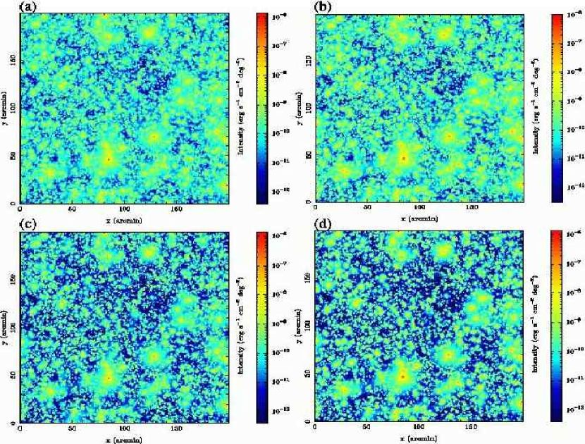
Figure 4.— The simulated $200\arcmin\times 200\arcmin$ region in four energy bands: (a) 250 – 350 eV; (b) 350 – 425 eV; (c) 550 – 600 eV; (d) 700 – 800 eV. Emission lines from C, N, O, and Fe dominate in each band, respectively.

To study the spectroscopic properties of the soft X-ray emission from the WHIM gas, we divide the simulated patch of sky into $40\times 40$ grid cells, with each cell extending over an area of $5\arcmin\times 5\arcmin$ . In every cell, we obtain the X-ray spectrum of each gas particle by applying the Raymond-Smith code, based on its temperature, density, metallicity and redshift. The peculiar velocities of the gas particles are used in order to produce a redshift space spectrum. We then combine all the spectra to obtain a synthesized spectrum in each cell, as mentioned above.

Figure 5 shows 10 random samples of such spectra picked from the brightest 10 % of pixels over the range 0.3–0.9 keV. A large number of emission lines are visible in many of the panels. Having information from the underlying simulation allows us to identify lines easily. Our scheme for doing this automatically is as follows. When creating the spectra, for each energy bin, we keep track of the redshift of the particle that was the largest contributor of X-ray flux to that bin. When plotting the spectra, we divide the energy of bin $i$ by $1+z_{i}$, where $z_{i}$ is the redshift of the maximum flux particle. If the resulting value is within 5 eV of one of the known ion rest wavelengths (see Table 1), and the pixel corresponds to a peak in the spectrum, we label it with the name of ion species, and the redshift $z_{i}$. It can be seen that many of the features come from the same redshift, but are signposted by different species. For example, the top left panel shows that a number of lines (N VII, O VIII, Fe XVII and Ne IX) arise from hot gas at redshift $\sim 0.35$. These types of spectra can potentially provide us with important information that could help us identify emission lines with ion species and redshifts in real observations.

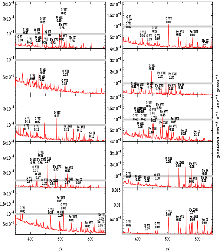
Figure 5.— 10 random sample spectra taken from the brightest 10% of pixels. Note that the y-axis scale changes between each plot. We have plotted a gray bar at count level $10^{-4}$ photons cm^-2 s^-1 pixel^-1 keV^-1 so that the panels can more easily be compared. The pixel size is $5\arcmin\times 5\arcmin$. The redshifts of material contributing to emission lines are shown

3.2. Contribution from the Galactic Foreground and AGNs

ROSAT (Snowden et al., 1995, 1997) and other X-ray missions (see, e.g., McCammon et al., 2002; Sanders et al., 2001) show that the soft X-ray background in the band 0.1 - 1 keV is comprised of at least three components: (1) unabsorbed X-ray emission, referred to as the ”local hot bubble” (LHB), from a cavity in the local interstellar medium (Snowden, 1998; Sfeir et al., 1999); (2) hotter absorbed X-rays, referred to as ”transabsorption emission” (TAE, Kuntz & Snowden, 2000; Snowden, Freyberg, Kuntz, & Sanders, 2000), from gas in either the Galactic halo or the intragroup medium of the Local Group (Rasmussen & Pedersen, 2001; Rasmussen, Kahn, & Paerels, 2003), and (3) an extragalactic X-ray background (Hasinger et al., 1998; Mushotzky, Cowie, Barger, & Arnaud, 2000). Simultaneous fits to ASCA and ROSAT data arrive at the same components (Miyaji et al., 1998).

It is well known that the extragalactic X-ray background is dominated by discrete sources such as active galactic nuclei (AGNs). ROSAT deep surveys resolved $\sim$70 – 80% of the soft X-ray background (0.5 – 2 keV) into discrete sources at a flux limit of $10^{-15}\rm\ erg\ cm^{-2}s^{-1}$ (Hasinger et al., 1998). The Chandra deep survey, which had a flux limit of $3\times 10^{-16}\rm\ erg\ cm^{-2}s^{-1}$, resolved an additional 6 – 13% into point sources (Mushotzky, Cowie, Barger, & Arnaud, 2000). This leaves room for $\sim$5 – 25% to come from diffuse emission from hot gas in the IGM, which is what we concentrate on in this paper.

To obtain the composite spectrum of the Galactic foreground and the AGN background, we use the following simple models of the components. (1) For the LHB, we adopt a thermal plasma model with k$T=0.1$ keV and emission measure $EM=0.019\rm\ cm^{-6}$ pc. The metal abundance is taken to be solar, except for Mg, Si, and Fe, which have an abundance of 0.28 $Z_{\odot}$. (2) For the TAE, we adopt a thermal plasma model with k$T=0.227$ keV and emission measure $EM=0.003\rm\ cm^{-6}$ pc. This model has solar abundances and is absorbed by a hydrogen column density of $N_{H}=1.8\times 10^{20}\rm\ cm^{-2}$. The parameters for these two thermal components were obtained from fits to the calorimeter sounding rocket data reported in McCammon et al. (2002) using the MEKAL spectral models in XSPEC . (3) The third component represents the AGN. We used a spectrum constructed by D. McCammon (private communication) to reflect all the known ROSAT and Chandra data on the resolved AGN contribution of the soft X-ray background (see Figure 15, McCammon et al., 2002). In Figure 6 we show the composite spectrum of these three components.

Figure 6.— Composite spectrum of the Galactic foreground and AGNs. It includes three components: (a) a thermal emission from the Local Hot Bubble; (2) an absorbed thermal emission from hot gas either in the distance halo or in the Local Group; and (c) continuum emission from discrete AGNs.

3.3. X-ray spectra of Characteristic Regions

We select three regions (shown as white boxes in Figure 3) to study three typical types of X-ray emission: (a) hot gas in a galaxy group (Figure 7a); (b) diffuse X-ray emission in a filament (Figure 7b); and (c) a void (Figure 7c). In each panel we show three curves: the red line is the emission from the IGM, green is the composite spectrum of AGNs and the Galactic foreground, and the black line represents the total emission. We also identify the most significant IGM emission lines with their ion species and redshifts in a similar fashion to Figure 5.

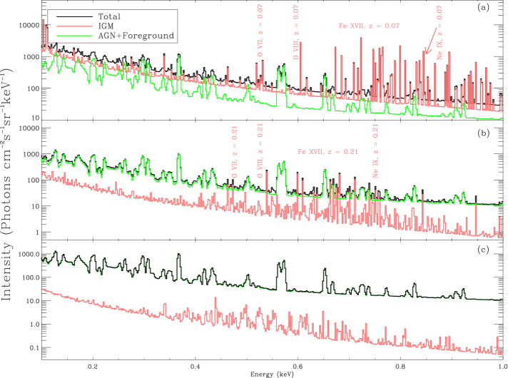
Figure 7.— Simulated spectra of three selected regions. Green lines are for the IGM emission, red lines are for the Galactic foreground plus AGNs, and black lines stand for total X-ray emission. (a) Hot gas in a galaxy group, it is clear that the IGM emission dominates the whole spectrum, especially at high energy; (b) diffuse X-ray emission in a filament; The Galactic foreground plus AGNs’ emission dominate, but some strong emission lines from a filament at $z\approx 0.21$ show up in the total spectrum; and (c) a void, in which the entire spectrum is dominated by the Galactic foreground plus AGNs. We also label redshifts of several selected lines.

In Figure 7a it is clear that the IGM emission dominates the entire spectrum. This is not surprising because the X-rays come from the hot gas within a galaxy group at redshift $z\approx 0.07$. For such hot gas, bremsstrahlung radiation, which dominates the total X-ray emissivity, is $\propto n_{e}^{2}T^{0.5}$, where $n_{e}$ is the electron density and $T$ is the temperature. The X-ray emission from the high density and high temperature intragroup medium shows a strong continuum, and this dominates over the AGN and Galactic foreground emission. In this panel we identify emission lines from O, Fe, and Ne. In particular we can easily make out redshifted O VIII Ly$\alpha$ (resonance line at 611 eV) and the O VII triplet (forbidden line at 524 eV, intercombination line at 531 eV, and resonance line at 536 eV). This could provide us with a direct measurement of the temperature, electron density and ionization states of this X-ray emitting gas. The numerous lines between 650 – 850 eV are mainly emission lines from Fe L-shell transitions, and many of these lines belong to Fe XVII transitions.

Figure 7b shows the emission spectrum of a patch of sky covered with more diffuse structures, known to be filamentary in 3 dimensions [area (b) in Figure 3]. The total spectrum (black line) is dominated by the background (AGNs) and foreground emission, especially at E $<0.4$ keV. However, we see several emission lines from a filament crossing the line of sight at $z\approx 0.21$. Although the overall continuum level is nearly an order of magnitude lower than that of the AGNs plus the foreground, these emission lines are strong enough to poke through the total spectrum and show up as obvious features.

In Figure 7c the total spectrum is completely dominated by the AGNs plus the foreground. The emission from the IGM is almost 100 times lower that that of the AGNs plus the foreground, and it is not possible to detect any signals from the IGM.

In Figure 8 and  9 we zoom in on areas (a) and (b), respectively, plotting only emission from gas which lies within particular narrow range in redshift (explained below). These plots have angular resolution four times higher than that in Figure 3. Figure 8 shows a simulated $20\arcmin\times 20\arcmin$ region, centered on area (a) (denoted by the white box). Most X-ray emission lines from this area originate from hot gas at $z\approx 0.0775$, so that we have cut out a slice that is centered on this redshift with $\Delta z=0.0005$ (about 1.5 comoving $h^{-1}{\rm Mpc}$). Figure 8 shows the X-ray emission from this slice, and the dotted lines show contours of X-ray emission. In similar fashion we have made Figure 9 for area (b). Clearly, the round shape of the X-ray contours in Figure 8 indicates that the hot gas in area (a) sits in a virialized, relatively stable system, such as a galaxy group. The X-ray contours in area (b) (Figure 9) (we are plotting only emission coming from close to $z=0.21$) show rather more diffuse and irregular X-ray emission from filamentary structures.

To further understand the gas distribution within area (a) and (b), we examine all the particles in these two areas centered around redshifts of $\sim$ 0.775 and 0.21, respectively. The length along the line of sight correspond to 5$\arcmin$ at that redshift, i.e., two cubes with comoving sizes $0.33h^{-1}\times 0.33h^{-1}\times 0.33^{-1}\,\rm Mpc^{3}$ at $z=0.775$ and $0.86h^{-1}\times 0.86h^{-1}\times 0.86^{-1}\,\rm Mpc^{3}$ at $z=0.21$. In Figure 10 we plot the temperature vs. overdensity of gas particles with $T>10^{5}$ K. Red filled circles represents particles in area (a), and black ones are from area (b). In area (a), most particles concentrate on a region with overdensities around $10^{3}$, while in area (b) gas particles distribute more diffusely. The confirms our initial guess that particles in area (a) are more concentrated and tend to form a virialized structure, and in area (b) structure is more filamentary-like.

Clearly, an important method to distinguish between area (a) and (b) is to study the emission line strength via, i.e., Figure 7. But exactly how does the observed line strength vary with gas density? To understand this, we select O VIII line at 654 eV as a representative line and study the line flux in each of the $5\arcmin\times 5\arcmin$ grid. Again we select all the grids around the two redshifts, 0.0775 and 0.21, to calculate the O VIII flux from each cube. The total flux of O VIII emission line from one cube can be obtained by direct summarization of the line flux from each individual particle in that cube (Yoshikawa et al., 2003). The mean density of that cube is calculated by averaging the total mass of particles with $T>10^{5}$ K within that cube. Figure 11 shows the line flux distribution for both regions: red filled circles represent cubes at redshift of $\sim 0.0775$, and black filled circles are from cubes at $z\sim 0.21$. Two circles pointed by arrows are area (a) and (b). While the line flux dependency on gas density is a complicated relation because it involves properties like temperature, ionization structure and metallicity, in general Figure 11 shows that high density regions tend to have high O VIII fluxes. We also calculate the flux sensitivity of the proposed X-ray mission MBE (the horizontal dashed line) for a 200 ksec exposure time. While only very few girds in this plot are detectable with MBE at the two redshifts, the cumulative effect by observing each grid up to higher redshifts greatly enhances the overall detectability (see discussion in section §5).

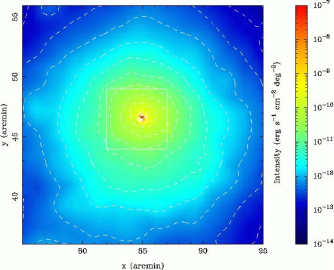
Figure 8.— A slice of the simulated region, centered on area (a) (white box), with a size of $20\arcmin\times 20\arcmin$. The slice is a projection of $\Delta z=0.0005$, centered at $z\approx 0.0775$. The X-ray contours are separated by a factor of $\sim$ 2.2 in intensity, with the highest contour at a level of $\sim 10^{-7}\rm\ ergs\ s^{-1}cm^{-2}deg^{-2}$.

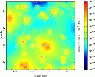
Figure 9.— Same as Figure 8, but enlarged area (b) (white box at the center). The slice is a projection of $\Delta z=0.0005$, centered at $z\approx 0.2108$. The X-ray contours are separated by a factor of $\sim$ 3.5 in intensity, with the highest contour at a level of $\sim 10^{-9}\rm\ ergs\ s^{-1}cm^{-2}deg^{-2}$.

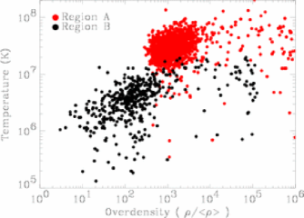
Figure 10.— Temperature vs. overdensity of gas particles with $T>10^{5}$ K in area (a) and (b). Red filled circles represents particles in area (a), and black ones are from area (b).

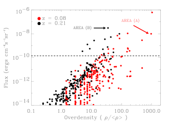
Figure 11.— O VIII line flux vs density in each cube at redshift 0.0775 (red) and 0.21 (black) in our $200\arcmin\times 200\arcmin$ simulation. We also label the two areas (a) and (b). The dashed horizontal line is the estimated flux sensitivity of the proposed X-ray mission MBE for a 200 $ksec$ exposure time.

4. Correlation

4.1. Angular Clustering of the WHIM

As most of the emission from the WHIM comes from relatively low redshifts, z $<$ 0.3, the strong spatial clustering of the baryons on small scales is directly reflected in strong angular clustering of their X-ray emission. In Figure 12 we show a map of a region of sky of angular size $10\arcdeg\times 10\arcdeg$ taken from our hydrodynamic simulation. The image is taken in the energy band from 0.5 – 0.8 keV, and includes an AGN contribution and a galactic foreground component (both smoothly distributed). The mean flux from AGN plus foreground is $\sim 4\times 10^{-12}\rm\ ergs\ cm^{-2}s^{-1}deg^{-2}$, which we obtained by integrating the model from Figure 6 between 0.5 – 0.8 keV. The map has been smoothed with a filter of Gaussian width $\sigma=5\arcmin$. In the map, emission from many groups of galaxies can be seen as hotspots, as well as more diffuse emission between them.

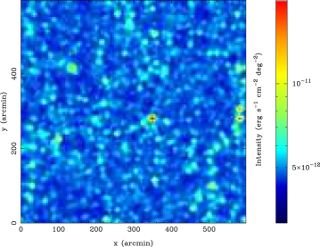
Figure 12.— A simulation of $10\arcdeg\times 10\arcdeg$ region. The image is an integration of the total spectrum (IGM plus Galactic foreground plus AGNs) between 0.5 – 0.8 keV. The map has been smoothed with a filter of Gaussian width $\sigma=5\arcmin$. In the map, emission from many groups of galaxies can be seen as hotspots, as well as more diffuse emission between them.

The angular clustering of the WHIM emission is treated more extensively in Croft et al. (2001). In this paper we show an angular map with a larger scale, and in a narrower band. It is evident that the WHIM is strongly clustered. We compute the angular correlation function $w(\theta)$ from this map, where $w(\theta)$ is defined as:

$$w(\theta)\equiv\left<\delta_{X}(\alpha)\delta_{X}(\alpha+\theta)\right>$$ (2)

Here $\delta_{X}(\alpha)$ is the X-ray flux over the mean: $\delta_{X}\equiv f_{X}/\left<f_{X}\right>-1$ where $f_{X}$ is the X-ray flux in each pixel between 0.5 – 0.8 keV. We look at three types of X-ray emission auto-correlation function: X-rays from WHIM only, in which we solely use gas particles with temperatures between $10^{5}$ – $10^{7}$ K; X-rays from the emission lines only, for which we subtract the continuum from the total spectrum; and X-rays from the IGM. All three types exhibit a strong clustering signal at high significance (see Figure 13). This strong clustering is an obvious signature of the IGM. Photons from AGN originate from much farther away and their angular clustering is predicted to be smaller on these scales (see e.g., Croft et al., 2001). Even with only one such field, the IGM signal shows up very well.

Figure 13.— Angular auto-correlation function calculated from Figure 12. X-ray emission has been integrated from 0.5 – 0.8 keV. Open triangles represent X-ray emission from the WHIM gas ($10^{5}<\rm T<10^{7}$ K), open circles are for emission lines only, and filled circles are for X-ray emission from all of the IGM.

4.2. Cross-correlation of the IGM Emission and Galaxy Positions

Numerical simulations show that the X-ray emission from the IGM traces the same large scale structures as galaxies. By calculating the angular cross-correlation of the X-ray background (XRB) with nearby galaxies in simulated surveys of $1\arcdeg\times 1\arcdeg$ fields, Croft et al. (2001) found a strong signal on an angular separations of $\theta<5\arcmin$ (see their Figure 13a). Since the X-ray emissivity is $\propto n_{e}^{2}T^{\alpha}$, and the temperature is roughly proportional to the density for WHIM gas (Davé et al., 2001), it is obvious that the large scale pattern of X-ray emission should correlate well with that of baryonic overdensity $\delta$. Moreover, based on the assumptions in our simulation, the highly ionized metals can be directly related to local matter overdensities, so that we expect a strong correlation between emission lines from metals and nearby large scale structures. In this section, we will test the idea that correlation of spectral pixel fluxes with the positions of galaxies will enable us to detect the presence of the WHIM.

We first identify galaxies in the simulation using the SKID groupfinder (see, e.g., Katz, Weinberg, & Hernquist, 1996). The galaxies are then used to create a mock redshift survey occupying the same simulation space as the X-ray emission. This part of the procedure is similar to that employed in Croft et al. (2001), and we also produce a flux limited survey of galaxies. We adjust the magnitude limit so that the mean redshift of the galaxies is $z=0.2$. We apply an upper redshift cutoff to our sample at $z\leq 0.5$, because most X-ray emission from the hot IGM comes from low redshift. The simulated sky area which we explore in this section has a size of $200\arcmin\times 200\arcmin$, and the redshift survey contains 57,607 galaxies.

We divide the $200\arcmin\times 200\arcmin$ field into a $200\times 200$ grid, with each cell subtending $1\arcmin\times 1\arcmin$. We calculate the total spectrum in each cell, accumulating emission from a redshift up to $z\sim 0.5$, and using a spectral resolution of 2 eV.

Our analysis technique involves first subtracting the continuum from the spectrum to obtain an emission-line only spectrum. We do this using an iterative technique to lower the emission line profile to the level of the continuum, without using knowledge of the true continuum. To study the cross-correlation between galaxies and the X-ray emission lines from different ion species, for each ion species at a time, we remap all the energy bins in the spectrum, which contains emission lines from all ion species, to redshifts, based on the rest energy of that particular ion species. For instance, to examine the cross-correlation between the O VIII emission lines and nearby galaxies, we set the zero-redshift point of each spectrum, which contains emission lines from all ion species, to $E_{0}=654$ eV. The redshift $z_{i}$ of spectral bin with energy $E_{i}$ is assigned according to $z=E_{0}/E_{i}-1$. Then for each spectral bin with energy $E_{i}$, we have a corresponding redshift $z_{i}$ and two-dimensional angular coordinate. We then use the redshifts of the spectral bins and their angular positions on the sky to give each spectral bin a three-dimensional comoving Cartesian coordinate (making use of the appropriate relations for our $\Lambda$CDM cosmology.) We define the cross-correlation function $\xi_{c}(R)$ to be:

$$\xi_{c}(R)\equiv\left<I_{X}(r)\delta_{g}(r+R)\right>.$$ (3)

Here $I_{X}$ is the X-ray intensity in each spectral bin after continuum subtraction, in units of $\rm photons\ cm^{-2}s^{-1}sr^{-1}keV^{-1}$, and $\delta_{g}$ is the galaxy overdensity. $\xi_{c}(R)$ therefore has units $\rm photons\ cm^{-2}s^{-1}sr^{-1}keV^{-1}$.

Figure 14 shows the cross-correlation functions for eight ion species. During the calculation, the zero-redshift points were set to the corresponding rest-frame energies, as mentioned above. For He-like ions, we chose the rest resonance energies, and for Fe XVII we let $E_{0}=825.79$ eV. The 1-$\sigma$ error bars are obtained by splitting the dataset into 20 subsamples, and calculating the standard deviation of these 20 subsamples. It is apparent that for all the ions except C V and N VI, there are strong signals at small distances, which we interpret to mean that these X-ray emission lines are strongly correlated with large scale structures traced by galaxies. In regions close to galaxies, these signals, after subtracting their mean values at large distances (by analogy with the galaxy or matter correlation function), can be fitted with power laws with slopes ranging between -1.2 – -2. Since hot galactic halo gas lies typically within scales less than a few hundred Kpc from galaxies, we can identify these signals as the correlation signals of hot gas in the IGM and galaxies. If we do not subtract the mean value of $(\xi_{c})$ from the results, the $\log(\xi_{c})$ – $\log(R)$ relation can be approximately fitted by a power law over the entire range. Fe XVII and O VIII show the steepest power law slopes of $\sim$ (-0.43), while O VII, N VII, and C VI show slopes between (-0.33) – (-0.30). Ne IX has a rather flat slope of $\sim$ (-0.15).

Figure 14.— Cross-correlation between the IGM emission lines and galaxies: (a) Ne IX and Fe XVII, (b) O VII and O VIII, (c) N VI and N VII, (d) C V and C VI. These IGM emission lines (except N VI and C V) tend to cluster around galaxies at scales $\lesssim$ 1 – 2 Mpc.

It is interesting to see that different ions show different characteristic correlation strengths. The strongest signal comes from O VIII and Fe XVII. O VII and Ne IX also show a relatively strong signal, whereas C VI and N VII give a weak signal, while C V and N VI are not detected at all. This can be explained by the combination of ion emissivity and element abundance. From our definition, the correlation function $\xi_{c}(R)$ should be a function of $(\epsilon_{i}Z_{i})$, where $\epsilon_{i}$ is the line emissivity for ion $X_{i}$, and $Z_{i}$ is its elemental abundance. The higher $(\epsilon_{i}Z_{i})$, the larger the $\xi_{c}(R)$. From Figure 1, O VIII (solid blue-green curve) and Fe XVII (dotted green curve) show the highest peak emissivities, so they have the highest correlation signals. However, since oxygen is more abundant than iron, O VIII gives a stronger signal, even compared to Fe XVII. Following a similar line of argument, we can explain the relative strengths of the correlation signal from the other ions.

Different ions are detectable over different scales, depending on the strength of the emission. The correlation signal for O VIII can be seen strongly for $R\leq 2$ Mpc, while others (namely O VII, Fe XVII, Ne IX and C VI) only start to show an obvious signal at $R<1$ Mpc, with N VII only tentatively seen, at an even smaller scales. For highly overdense regions, which typically also have large galaxy overdensities, even on relatively large scales, the high elemental abundance and large emissivity gives a significant signal for O VIII; while for other ions, the lower abundances and/or lower emissivities mean that the signal is only readily seen within short distances from the overdense area, say, $R<1$ Mpc.

5. Detectability

Generally, most emission lines from the filaments are weak, undetected by current X-ray telescopes. These lines are expected to be embedded in the strong continuum emission from AGNs plus the Galactic foreground (see Figure 7). To investigate their detectability, we define the equivalent width of an emission line at energy $E$ as

$$EW\equiv\int_{E-\Delta E/2}^{E+\Delta E/2}\left(\frac{I}{I_{c}}-1\right)dE,$$ (4)

where $I$ and $I_{c}$ are the observed spectrum and its continuum, respectively, in units of $\rm photons\ cm^{-2}s^{-1}keV^{-1}sr^{-1}$. The integration is over a small energy range $\Delta E$ around $E$. For a weak emission line, $EW\ll\Delta E$. Given an exposure time of $T$, the minimum detectable equivalent width is

$$EW\geq\left(\frac{S}{N}\right)\left(\frac{E}{I_{c}RA\Omega T}\right)^{\frac{1}{2}}.$$ (5)

Here $(S/N)$ is the desired signal-to-noise ratio, $R$ is the instrumental resolving power, $A$ is the effective area and $\Omega$ is the solid angle over which the emission is integrated.

It is apparent, from equation (5), that an instrument with high $(RA\Omega)$ is needed to detect weak emission features. Current X-ray telescopes, such as the Chandra X-ray Observatory and the X-ray Multi-Mirror Mission (XMM-Newton) , have unprecedented spectral and spatial resolution. However, the detectors on board these telescopes either have high spectral resolution but low effective area, or large effective area but low resolving power, and thus are inadequate for achieving high resolution spectroscopy of extended structures that we are interested in.

Several proposed and planned X-ray missions have a large combined $(RA\Omega)$ and will show promise in detecting weak emission features from extended structures. We now examine four future X-ray missions, namely Astro-E2 , Constellation-X , The X-Ray Evolving Universe Spectrometer (or XEUS ), and the Missing Baryon Explorer (or MBE ). These X-ray missions are either in the final stage (Astro-E2), in planning stage (Constellation-X,XEUS), or in proposal stage (MBE). In particular, we will concentrate on MBE, a mission specifically designed to detect diffuse X-ray emission from the WHIM, to see how this can be achieved.

Table 2 gives the relevant parameters for these four instruments. In calculating the $EW$, we assume that the desired S/N ratio is 3, that the line has energy 0.6 keV (where most O and Fe lines lie), and that the exposure time is 200 ksec. Since the observed spectrum is dominated in most cases by the emission from the Galactic foreground and the AGN background, we adopt the continuum value $I_{c}\approx 24\ \rm photons\ cm^{-2}\ s^{-1}sr^{-1}keV^{-1}$ from Figure 6. We assume that we will devote a time, T, for each telescope to observe a region of sky of solid angle, $\Omega$, and we calculate the minimum $EW$ of detectable emission lines integrated over a solid angle, $\Omega_{PIXEL}$. When a telescope with a field of view, $\Omega_{FOV}$, maps a region with solid angle, $\Omega$, with a total exposure time, T, each point of the region receives a exposure time of $(T\times\Omega_{\rm FOV}/\Omega)$, so the minimum EW in each pixel can be expressed as:

$$EW\geq\left(\frac{S}{N}\right)\left(\frac{\Omega E}{I_{c}RAT\Omega_{\rm FOV}\Omega_{\rm PIXEL}}\right)^{\frac{1}{2}}.$$ (6)

To compare the minimum detectable $EW$ among the four instruments, we use as the value for $\Omega_{PIXEL}$ the largest instrument pixel size ($4.9\arcmin\times 4.9\arcmin$ from MBE), and for $\Omega$ we take the largest instrument field of view ($29.5\arcmin\times 29.5\arcmin$ from MBE). In the case of the same $\Omega$, $\Omega_{PIXEL}$, and T, equation (5) indicates that the instrument with the largest value of $RA\Omega_{FOV}$ gives the smallest $EW$, as indicated in the last two columns of Table 2. Although XEUS has much higher angular resolution than MBE, its smaller instrument pixel size offers no advantage in detecting faint diffuse emission lines, unless the relevant scale of angular structure is significantly smaller than the MBE pixel size. The large field of view of MBE makes it clearly the best-suited mission for detecting weak X-ray emission lines from extended sources.

Table 2: Instrument Parameters and Detection Limits
Instrument	$A$	$\Omega_{\rm FOV}$	$\Omega_{\rm PIXEL}$	$R$	$RA\Omega_{\ rmFOV}$	$EW$
	$\rm(cm^{2})$				$(\rm cm^{2}deg^{2})$	(eV)
Astro-E2 1	35	$2.9\arcmin\times 2.9\arcmin$	$0.48\arcmin\times 0.48\arcmin$	100	5	138.0
Constellation-X 2	3,000	$2.5\arcmin\times 2.5\arcmin$	$5\arcsec\times 5\arcsec$	400	2,083	8.0
XEUS 3	40,000	$1\arcmin\times 1\arcmin$	$2\arcsec\times 2\arcsec$	500	5,556	4.9
MBE	300	$29.5\arcmin\times 29.5\arcmin$	$4.9\arcmin\times 4.9\arcmin$	150	10,878	3.7

1. XRS: the X-ray Spectrometer
2. SXT: the Spectroscopy X-ray Telescope
3. STJ I: the initial configuration for the Superconducting Tunneling Junctions.

MBE is a mission designed specifically to observe the X-ray emission from the warm-hot, moderate overdense gas predicted to be distributed in filamentary structures that connect collapsed, virialized regions such as groups and clusters of galaxies. It will also be well suited for detailed studies of emission lines from groups themselves. It consists of a single instrument, the X-ray Calorimeter Telescope (XCT) – a high-resolution spectrometer and a moderate resolution imager. The energy resolution is $\sim$ 4 eV (FWHM), with an energy bandpass from 40 — 2000 eV. The field of view consists of a $6\times 6$ array of pixels $\sim\ 4.9\arcmin$ on a side, so that the field of view is $29.5\arcmin\times 29.5\arcmin$.

In Figure 15 we show a simulated MBE count map of the same $10\arcdeg\times 10\arcdeg$ field shown in Figure 12. The energy band plotted is between 500 – 800 eV. The total exposure time required to build up such an image is $\sim$4 Msec, consisting of 400 pointings of 10 ks each. We add photons from AGNs plus the Galactic foreground, with a mean count of $\sim 80$ counts $\rm pixel^{-1}$. We also add Poisson-distributed noise to the map. During such a short exposure time, the counts collected in each pixel range from $\sim$ 80 – 90 counts $\rm pixel^{-1}$, for pixels which contain purely background/foreground emission, up to $\sim 350$ counts $\rm pixel^{-1}$, arising from hot spots such as galaxy groups.

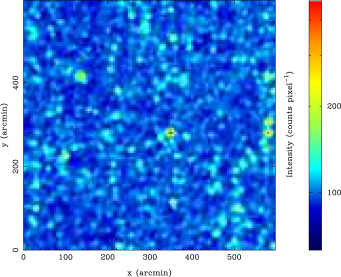
Figure 15.— MBE view of the same area shown in Figure 12. The total exposure time is $\sim$4 Msec. A Poisson-distributed noise was added. AGNs plus the Galactic foreground contribute a mean count of $\sim 80$ counts $\rm pixel^{-1}$

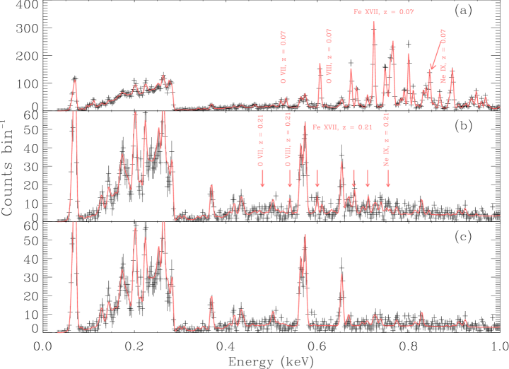
Figure 16.— Simulated spectra observed with MBE response functions. The three spectra correspond to the three regions labeled in Figure 3, respectively. The exposure time is 200 ksec for each spectrum. In panel (b), it is clear that MBE should be able to probe several weak X-ray emission lines from filaments.

To demonstrate how MBE can detect weak X-ray emission features, we also present the instrumental-folded spectra of the three areas we discussed previously (see Figure 16). To obtain these spectra, we used the software package ISIS (Interactive Spectral Interpretation System, see Houck & Denicola, 2000) , and applied the instrumental response data and effective area data for MBE. The three panels in Figure 16 represent spectra for the three regions we have examined before. The red lines are the model spectra, and the black crosses represent observations of these spectra. The errors bars on each point are based on 1-$\sigma$ Poisson statistics only. The binsize is 2 eV and the exposure time is 200 ksec. We label the ion species and their redshifts in red text. It is clear that many weak emission lines, particularly in Figure 16b, where the emission is from a filament, can be detected without ambiguity. For instance, the emission line from the $z\approx 0.21$ O VIII line contains nearly 30 counts.

An interesting question to ask is what fraction of the sky as probed by MBE can yield detectable weak emission lines such as those in Figure 16b, given a certain amount of exposure time? This we have calculated by examining the 1,600 spectra from the $200\arcmin\times 200\arcmin$ sky simulation. For most WHIM emission, the continuum should be dominated by the AGN plus Galactic foreground emission. Taking oxygen lines as an example, assuming most weak emission lines seen in Figure 7a span only one bin, which has a binsize of 2 eV, to ensure a 4-$\sigma$ detection in one pixel, the signal in the line, as a function of exposure time T, should be at least

$$S=1.85\times 10^{-2}\ T^{\frac{1}{2}}\ \rm counts,$$ (7)

and the line peak intensity, also as a function of exposure time T, should be at least

$$I_{peak}=2\times 10^{4}\ T^{-\frac{1}{2}}+24\ \rm photons\ cm^{-2}s^{-1}keV^{-1}sr^{-1}.$$ (8)

Assuming an exposure time for each pixel, we can then convert this line peak intensity to line flux sensitivity. Taking $T=200\ ksec$ as an example, the flux sensitivity at the energy of O VIII would then be $1.4\times 10^{-10}\rm ergs\,cm^{-2}s^{-1}sr^{-1}$. This is shown as the horizontal dashed line in Figure 11. Typically MBE would be able to probe regions with overdensities around 100. In the $200\arcmin\times 200\arcmin$ sky simulation, we can then count the total number of angular grid cells for which the spectra show at least one line with peak intensity $\geq I_{peak}$. The fraction of the sky is obtained by dividing this number by the total number of angular grid cells, which is 1,600 in this case. Figure 17 plots that fraction of the sky as a function of exposure time. The errors on the points are based on 1-$\sigma$ poisson fluctuations only. We can see from this that for one 200 $ksec$ observation with MBE, given the field-of-view of $\sim 900$ square arcmin, roughly $\sim$ 5% of the field-of-view, or 2 pixels will show detectable emission lines.

Figure 17.— The fraction of the sky probed by MBE with at least one detectable (4$\sigma$) weak emission line, given the exposure time T. The errors are based 1-$\sigma$ poisson fluctuation only.

6. Discussion and Summary

We have presented a detailed study of predictions for the soft X-ray emission from the Warm-Hot Intergalactic Medium. Our main conclusions can be summarized as follows:

1. We have examined images of soft X-ray emission from the hot IGM with a wide field of view ($200\arcmin\times 200\arcmin$). Having spectral information for each pixel allowed us to view the sky in several different soft X-ray energy bands, where emission lines from different ion species dominate. The low energy emission is markedly more diffuse than X-rays in the higher bands.

2. We selected three representative simulated patches of sky to study with high resolution X-ray spectra: (a) a galaxy group; (b) a filament; (c) a void-like, underluminous region. In each case, we saw numerous emission lines from elements such as C, N, O, Fe, Ne, and identified their redshifts.

3. By taking into account the background X-ray emission from the AGNs and foreground emission from the Galaxy, we obtained composite X-ray spectra of the selected regions. We found that in areas where the galaxy group is present, the X-ray spectrum is dominated by the hot intragroup medium, while in the void-like areas, the spectrum is completely dominated by the AGNs plus the Galactic foreground. In the filament case, although the majority emission comes from the AGNs plus the Galactic foreground, it is still possible to detect strong emission lines from the WHIM.

4. We found that the emission in the (0.5-0.8 keV) band (covering many of the emission lines) shows strong small scale angular clustering, as measured by the angular autocorrelation function. Also, spectral information for each pixel allowed us to measure three dimensional clustering. In particular, we computed the cross-correlation between eight different ion species and the simulated galaxy distribution. We found that O VIII showed the strongest correlation signal, being measurable on scales as large as $\sim 4-5h^{-1}$ Mpc, while low energy species such as C V and N VI showed no correlation at all. This variation of the correlation strengths can be explained by ($\epsilon_{i}Z_{i}$), the combination of line emissivity $\epsilon_{i}$ and elemental abundance $Z_{i}$: the larger ($\epsilon_{i}Z_{i}$), the stronger the correlation signal.

5. Finally, we studied the detectability of the WHIM with several proposed X-ray missions. By comparing the effective area, resolving power and instrumental field-of-view, we found that the Missing Baryon Explorer ($\sl MBE$) shows the most promise for detecting weak emission lines from the WHIM gas. We also showed simulated MBE instrument-folded spectra of our three selected patches of sky.

Accurate prediction of the soft X-ray emission depends on several important factors, including X-ray emissivity, ionization fraction, metal abundances, etc. The largest uncertainty in our predictions of the soft X-ray emission comes from the metal abundance in the IGM. Theoretically, simulations are beginning to address the formation and distribution of metals in a self consistent way (see e.g., Cen & Ostriker, 1999; Springel & Hernquist, 2003; Aguirre et al. 2001a,b,c). The metallicity-density relationship we adopted in this paper was motivated by this work, and future studies of UV and soft X-ray emission lines should examine the question of metal enrichment in more detail (see, e.g., Furlanetto et al., 2003).

Observationally, metals are known to be distributed in a variety of systems with large dispersion in metallicity $Z$. For example, the metallicity can be as high as $10Z_{\odot}$ in the central regions of some active galactic nuclei (AGNs) (Mushotzky, Done & Pounds, 1993; Tripp, Lu & Savage, 1997), and as low as $10^{-3}Z_{\odot}$ in some halo stars in our galaxy (Beers, 1999). When we focus on the low redshift IGM, the main evidence for an enriched IGM comes from the observations of the X-ray-emitting gas within galaxy clusters (Mitchell et al., 1975; Mushotzky et al., 1996; Mushotzky & Loewenstein, 1997; Dupke & White, 2000). With ASCA, Mushotzky et al. (1996) found that the metallicities in four clusters vary between $0.3-0.5Z_{\odot}$. Studying $\sim 40$ clusters at $z>0.14$, Mushotzky & Loewenstein (1997) concluded that there is no metallicity evolution in clusters up to $z\sim 0.3$. The observations of the Ly$\alpha$ systems at low redshifts give metallicities as high as $\sim 0.05Z_{\odot}$ (Barlow & Tytler, 1998) indicating a metal enrichment in even lower density systems at low redshifts. The observations of damped Ly$\alpha$ systems [N(H I) $>10^{20}\rm\ cm^{-2}$] show a similar result (de la Varga et al., 2000). Due to the lack of observations, the metallicity of the “WHIM” is unknown.

Another uncertainty comes from the sensitive dependence of the X-ray emissivity and ionization fraction on physical properties of the WHIM gas, such as its temperature and density. For instance, both the emissivity and ionization fraction peak over a rather narrow range of temperatures, and drop rapidly at low and high temperatures (see Figure 1 and Figure 2, 3, & 4 of Chen, Weinberg, Katz, & Davé, 2003), which means a small change in temperature will cause order-of-magnitude changes in both quantities. This will in turn cause a dramatic change in observables such as intensity and emission line ion species. Because of this the actual observed spectrum depends sensitively on the underlying physical properties of the WHIM gas.

In this paper, we adopted several approximations to simply the calculations. First we did not take into account photoionization – we used collisional ionization when calculating the ionization fractions. It is important to be aware that photoionization from background radiation may substantially alter the metal ionization fractions for low density, low temperature gas (see, e.g., Chen, Weinberg, Katz, & Davé, 2003), which in turn will change the observed spectrum. However, since most of the emission spectra that can be observed with MBE or other telescopes are produced by hot gas in the high density, high temperature tail of the WHIM distribution, where collisional ionization dominates, we expect that photoionization will not substantially change those observables.

Metal cooling is ignored in our simulation: the cooling is primarily through H and He. Metal line cooling could be very important in some cases, especially for high density, warm/hot gas (see, e.g., Sutherland & Dopita, 1993). However, since our results are very sensitive to the temperature variation, it is important to quantify the possible effect of metal cooling on WHIM gas temperature. To cool some hot gas, giving it a small drop in temperature $\delta T$, the characteristic time scale $\delta t$ is

$$\delta t=\alpha\frac{k}{n\Lambda(T)}\delta T.$$ (9)

Here $\alpha$ is $3/2$ or $5/2$, depending on whether the cooling is isochoric or isobaric; $k$ is Boltzmann’s constant; $n$ is the electron density; and $\Lambda(T)$ is the cooling function. Assuming that we are interested in how cooling acts on timescale of order the Hubble time, we can estimate the effect of metal cooling on the temperature decrement $\delta T$ in terms of the physical parameters of the WHIM gas:

$$\delta\log T\approx 0.1\ n_{-5}\Lambda_{-23}T^{-1}_{6}\delta t_{\rm Hubble},$$ (10)

where $n_{-5}=n/(10^{-5}\ \rm cm^{-3})$; $T_{6}=T/(10^{6}\ \rm K)$; $\delta t_{\rm Hubble}$ is the cooling time in units of Hubble time scale. Here $\Lambda_{-23}$ is cooling rate in units of $10^{-23}\ \rm ergs\ cm^{3}s^{-1}$, typical of the WHIM gas with 0.1 solar abundance (Sutherland & Dopita, 1993). So in general, metal cooling has only a minor effect on our results; however, since $\Lambda(T)\propto T^{-1}$ in the temperature range we are interested in, the metal cooling process is more efficient for low temperature gas, especially so when $\Lambda(T)$ reaches its peak at $T\approx 2\times 10^{5}$ K.

It has been known for quite some time that non-gravitational heating, and/or cooling processes can change the overall level of cosmological X-ray emission substantially (Pen, 1999; Wu, Fabian, & Nulsen, 2001; Voit & Bryan, 2001a). The energy deposited by supernovae in our simulations has little direct effect on the IGM. It is added as thermal energy to particles in high density regions and is radiated away quickly. Although the direct impact of feedback is therefore minimal, the cooling included serves to change the entropy distribution of gas near the centers of virialized objects and lower the overall level of emission. Other treatments of starburst energy such as those which involve giving wind particles kinetic energy so that they escape beyond galaxy and group virial radii into the IGM (e.g., Springel & Hernquist, 2003) are also likely to change the distribution of X-ray emitting gas. Different treatments of feedback have been shown by Bryan & Voit (2001) and Voit & Bryan (2001b) to change the pdf of X-ray surface brightnesses in the range which would affect the WHIM emission lines we focus on here. Varying the feedback model would be useful in the future in order to assess the range of effects on the WHIM emission.

Finally, the ionization state of the gas was calculated assuming ionization equilibrium. Non-equilibrium evolution of the ionization state can significantly change the ionization fraction (see, e.g., Edgar & Chevalier, 1986; Hicks & Canizares, 2001). The characteristic time scale for hot gas to reach ionization equilibrium, or the recombination time scale is $\sim(n\alpha_{rec})^{-1}$, where $\alpha_{rec}$ is the recombination rate. At a temperature of $\sim 10^{6}$ K, the recombination rate for O VII, for example, is $\sim 1.4\times 10^{-12}\ \rm cm^{3}s^{-1}$ (Shull & van Steenberg, 1982). Here we include contributions from both radiative and dielectronic recombination. Assuming $n\sim 10^{-5}\ \rm cm^{-3}$, typical of WHIM gas, the recombination time scale is $\sim$ 2 Gyrs, less than the Hubble time. However, we must keep in mind that most of the hot gas was shock-heated at low redshift, so it is very likely that a significant portion of the WHIM gas has not reached its recombination time scale and is in a non-equilibrium ionization state.

A reasonable question to ask is: given detected X-ray emission lines, how do we identify lines with ion species and redshifts? It is impossible to carry out line identification with a single line; however, by simultaneously observing multiple lines such as the O VII triplet and/or O VIII redshifted to the same degree, which is within the capability of the energy resolution of proposed X-ray missions such as MBE, we can easily identify lines with redshifts. In addition, measurements of the line ratios can provide direct temperature/density diagnostics for the ionized plasma (see, e.g., Vedder, Canizares, Markert, & Pradhan, 1986). Observations of soft X-ray emission lines have the potential to not only reveal the presence of the missing baryons but to give us detailed information on their clustering, temperature, and metallicity.

X-ray emission provides a direct probe of the WHIM gas. Unlike the X-ray absorption method, which can yield only one dimensional information, by combining imaging/spectroscopic observations, X-ray emission can show us the fully three-dimension distribution of the WHIM gas. This is essential not only for closure of the local cosmic baryon budget, but also if we are to understand the distribution of the WHIM gas, and how structures form and evolve. Moreover, by applying line diagnostic methods, X-ray emission lines can be used to probe the metallicity, temperature and density of X-ray emitting gas. This in turn can give us important information on galaxy formation and evolution, given that most of these metals which are responsible for X-ray emission lines are produced by supernova explosions and propagate from the interstellar medium into intergalactic medium. Although the relatively low density and temperature make it hard to observe, currently proposed X-ray missions will for the first time provide us with detectable signals from the X-ray emission of the WHIM gas.

This work is supported by Carnegie Mellon University. T.F. thanks members of the astrophysics group at CMU for their help and stimulated discussions. T.F. also thanks to the hospitality of the Kavli Institute for the Theoretical Physics at the University of California, Santa Barbara, where part of the work was conducted. This research was supported in part by the National Science Foundation under Grant No. PHY99-0794.

References

- Aguirre et al. (2001a) Aguirre, A., Hernquist, L., Schaye, J., Katz, N., Weinberg, D. H., Gardner, J. 2001, ApJ, 560, 599
- Aguirre et al. (2001b) Aguirre, A., Hernquist, L., Katz, N., Gardner, J., Weinberg, D. H. 2001, ApJ, 556, L11
- Aguirre et al. (2001c) Aguirre, A., Hernquist, L., Schaye, J., Katz, N., Weinberg, D. H., Gardner, J. 2001, ApJ, 561, 521
- Barlow & Tytler (1998) Barlow, T. A. & Tytler, D. 1998, AJ, 115, 1725
- Beers (1999) Beers, T. C. 1999, Ap&SS, 265, 105
- Brown et al. (1998) Brown, G. V., Beiersdorfer, P., Liedahl, D. A., Widmann, K., & Kahn, S. M. 1998, ApJ, 502, 1015
- Bryan & Voit (2001) Bryan, G. L. & Voit, G. M. 2001, ApJ, 556, 590
- Cagnoni (2002) Cagnoni, I. 2002, astro-ph/0212070
- Cen et al. (1994) Cen, R., Miralda-Escudé, J., Ostriker, J.P., Weinberg, D. H., & Rauch, M. J. 1994, ApJ, 437, L9
- Cen, Kang, Ostriker, & Ryu (1995) Cen, R., Kang, H., Ostriker, J. P., & Ryu, D. 1995, ApJ, 451, 436
- Cen & Ostriker (1999) Cen, R. & Ostriker, J. P. 1999, ApJ, 514, 1
- Cen, Tripp, Ostriker, & Jenkins (2001) Cen, R., Tripp, T. M., Ostriker, J. P., & Jenkins, E. B. 2001, ApJ, 559, L5
- Chen, Weinberg, Katz, & Davé (2003) Chen, X., Weinberg, D. H., Katz, N., & Davé, R. 2003, ApJ, 594, 42
- Croft et al. (2001) Croft, R. A. C., Di Matteo, T., Davé, R., Hernquist, L., Katz, N., Fardal, M. A., & Weinberg, D. H. 2001, ApJ, 557, 67
- da Silva et al. (2000) da Silva, A. C., Barbosa, D., Liddle, A. R., & Thomas, P. A. 2000, MNRAS, 317, 37
- Davé, Dubinski, & Hernquist (1997) Davé, R., Dubinski, J., & Hernquist, L. 1997, NewA, 2, 71
- Davé, Hernquist, Katz, & Weinberg (1999) Davé, R., Hernquist, L., Katz, N., & Weinberg, D. H. 1999, ApJ, 511, 521
- Davé et al. (2001) Davé, R. et al. 2001, ApJ, 552, 473
- de la Varga et al. (2000) de la Varga, A., Reimers, D., Tytler, D., Barlow, T., & Burles, S. 2000, A&A, 363, 69
- Drake (1988) Drake, G. W. 1988, Can. J. Phys, 66, 586
- Dupke & White (2000) Dupke, R. A. & White, R. E. 2000, ApJ, 537, 123
- Edgar & Chevalier (1986) Edgar, R. J. & Chevalier, R. A. 1986, ApJ, 310, L27
- Fang & Bryan (2001) Fang, T. & Bryan, G. L. 2001, ApJ, 561, L31
- Fang et al. (2002) Fang, T., Marshall, H. L., Lee, J. C., Davis, D. S., & Canizares, C. R. 2002, ApJ, 572, L127
- Fang, Sembach, & Canizares (2003) Fang, T., Sembach, K. R., & Canizares, C. R. 2003, ApJ, 586, L49
- Furlanetto et al. (2003) Furlanetto, S. R., Schaye, J., Springel, V., & Hernquist, L. 2003, ApJ, submitted (astro-ph/0309736)
- Governato et al. (1997) Governato, F., Moore, B., Cen, R., Stadel, J., Lake, G., & Quinn, T. 1997, New Astronomy, 2, 91
- Gronenschild & Mewe (1978) Gronenschild, E. H. B. M. & Mewe, R. 1978, A&AS, 32, 283
- Hasinger et al. (1998) Hasinger, G., Burg, R., Giacconi, R., Schmidt, M., Trumper, J., & Zamorani, G. 1998, A&A, 329, 482
- Hernquist, Katz, Weinberg, & Jordi (1996) Hernquist, L., Katz, N., Weinberg, D. H., & Jordi, M. 1996, ApJ, 457, L51
- Hicks & Canizares (2001) Hicks, A. K. & Canizares, C. R. 2001, ApJ, 556, 468
- Houck & Denicola (2000) Houck, J. C. & Denicola, L. A. 2000, ASP Conf. Ser. 216: Astronomical Data Analysis Software and Systems IX, 9, 591
- Johnson & Soff (1985) Johnson, W. R. & Soff, G. 1985, Atomic Data and Nuclear Data Tables, 33, 405
- Kaastra et al. (2003) Kaastra, J. S., Lieu, R., Tamura, T., Paerels, F. B. S., & den Herder, J. W. 2003, A&A, 397, 445
- Katz, Weinberg, & Hernquist (1996) Katz, N., Weinberg, D. H., & Hernquist, L. 1996, ApJS, 105, 19
- Kuntz & Snowden (2000) Kuntz, K. D. & Snowden, S. L. 2000, ApJ, 543, 195
- Kuntz, Snowden, & Mushotzky (2001) Kuntz, K. D., Snowden, S. L., & Mushotzky, R. F. 2001, ApJ, 548, L119
- Markevitch et al. (2003) Markevitch, M. et al. 2003, ApJ, 583, 70
- Mathur, Weinberg, & Chen (2002) Mathur, S., Weinberg, D., & Chen, X. 2002, ApJ, 582, 82
- McCammon et al. (2002) McCammon, D. et al. 2002, ApJ, 576, 188
- McKernan et al. (2003) McKernan, B., Yaqoob, T., Mushotzky, R., George, I. M., & Turner, T. J. 2003, ApJ, 598, L83
- Mewe & Gronenschild (1981) Mewe, R. & Gronenschild, E. H. B. M. 1981, A&AS, 45, 11
- Mitchell et al. (1975) Mitchell, R. J., Charles, P. A., Culhane, J. L., Davison, P. J. N. & Fabian, A. C. 1975, ApJ, 200, L5
- Miyaji et al. (1998) Miyaji, T., Ishisaki, Y., Ogasaka, Y., Ueda, Y., Freyberg, M. J., Hasinger, G., & Tanaka, Y. 1998, A&A, 334, L13
- Mushotzky et al. (1996) Mushotzky, R.F., Loewenstein, M., Arnaud, K.A., Tamura, T., Fukazawa, Y., Matsushita, K., Kikuchi, K. & Hatsukade, I. 1996, ApJ, 466, 686
- Mushotzky, Cowie, Barger, & Arnaud (2000) Mushotzky, R. F., Cowie, L. L., Barger, A. J., & Arnaud, K. A. 2000, Nature, 404, 459
- Mushotzky, Done & Pounds (1993) Mushotzky, R. F., Done, C. & Pounds, K. A. 1993, ARA&A, 31, 717
- Mushotzky & Loewenstein (1997) Mushotzky, R.F. & Loewenstein, M. 1997, ApJ, 481, 63
- Nicastro et al. (2002) Nicastro, F. et al. 2002, ApJ, 573, 157
- Pearce et al. (2000) Pearce, F.R., Thomas, P.A., Couchman, H.M.P, & Edge, A., 2000, MNRAS, 317, 1029
- Pen (1999) Pen, U. 1999, ApJ, 510, L1
- Penton, Shull, & Stocke (2000) Penton, S. V., Shull, J. M., & Stocke, J. T. 2000, ApJ, 544, 150
- Phillips, Ostriker, & Cen (2001) Phillips, L. A., Ostriker, J. P., & Cen, R. 2001, ApJ, 554, L9
- Rasmussen, Kahn, & Paerels (2003) Rasmussen, A., Kahn, S. M., & Paerels, F. 2003, ASSL Vol. 281: The IGM/Galaxy Connection. The Distribution of Baryons at z=0, 109
- Rasmussen & Pedersen (2001) Rasmussen, J. & Pedersen, K. 2001, ApJ, 559, 892
- Raymond & Smith (1977) Raymond, J. C. & Smith, B. W. 1977, ApJS, 35, 419
- Sanders et al. (2001) Sanders, W. T., Edgar, R. J., Kraushaar, W. L., McCammon, D., & Morgenthaler, J. P. 2001, ApJ, 554, 694
- Savage, Tripp, & Lu (1998) Savage, B. D., Tripp, T. M., & Lu, L. 1998, AJ, 115, 436
- Scharf et al. (2000) Scharf, C., Donahue, M., Voit, G. M., Rosati, P., & Postman, M. 2000, ApJ, 528, L73
- Sfeir et al. (1999) Sfeir, D. M., Lallement, R., Crifo, F., & Welsh, B. Y. 1999, A&A, 346, 785
- Shull & van Steenberg (1982) Shull, J. M. & van Steenberg, M. 1982, ApJS, 48, 95
- Simcoe, Sargent, & Rauch (2002) Simcoe, R. A., Sargent, W. L. W., & Rauch, M. 2002, ApJ, 578, 737
- Snowden et al. (1995) Snowden, S. L. et al. 1995, ApJ, 454, 643
- Snowden et al. (1997) Snowden, S. L. et al. 1997, ApJ, 485, 125
- Snowden (1998) Snowden, S. L. 1998, Lecture Notes in Physics, v.506, Berlin Springer Verlag, 506, 103
- Snowden, Freyberg, Kuntz, & Sanders (2000) Snowden, S. L., Freyberg, M. J., Kuntz, K. D., & Sanders, W. T. 2000, ApJS, 128, 171
- Springel, White, & Hernquist (2001) Springel, V., White, M., & Hernquist, L. 2001, ApJ, 549, 681
- Springel & Hernquist (2002) Springel, V. & Hernquist, L. 2002, MNRAS, 333, 649
- Springel & Hernquist (2003) Springel, V. & Hernquist, L., 2003, MNRAS, 339, 289
- Sutherland & Dopita (1993) Sutherland, R. S. & Dopita, M. A. 1993, ApJS, 88, 253
- Tripp et al. (2001) Tripp, T. M., Giroux, M. L., Stocke, J. T., Tumlinson, J., & Oegerle, W. R. 2001, ApJ, 563, 724
- Tripp, Lu & Savage (1997) Tripp, T. M., Lu, L. & Savage, B. D. 1997, ApJS, 112, 1
- Tripp & Savage (2000) Tripp, T. M. & Savage, B. D. 2000, ApJ, 542, 42
- Tripp, Savage, & Jenkins (2000) Tripp, T. M., Savage, B. D., & Jenkins, E. B. 2000, ApJ, 534, L1
- Vedder, Canizares, Markert, & Pradhan (1986) Vedder, P. W., Canizares, C. R., Markert, T. H., & Pradhan, A. K. 1986, ApJ, 307, 269
- Voit & Bryan (2001a) Voit, G. M. & Bryan, G. L. 2001, Nature, 414, 425
- Voit & Bryan (2001b) Voit, G. M. & Bryan, G. L. 2001, ApJ, 551, L139
- Weinberg et al. (1997) Weinberg, D. H., Miralda-Escudé, J., Hernquist, L., Katz, N., 1997, ApJ, 490, 564
- Wu, Fabian, & Nulsen (2001) Wu, K. K. S., Fabian, A. C., & Nulsen, P. E. J. 2001, MNRAS, 324, 95
- Yoshikawa et al. (2003) Yoshikawa, K., Yamasaki, N. Y., Suto, Y., Ohashi, T., Mitsuda, K., Tawara, Y., & Furuzawa, A. 2003, PASJ, 55, 879
- Zhang, Anninos, & Norman (1995) Zhang, Y., Anninos, P., & Norman, M. L. 1995, ApJ, 453, L57