Microlensing signature of a white dwarf population in the galactic halo

Abstract

Microlensing and pixel-lensing surveys play a fundamental role in the searches for galactic dark matter and in the study of the galactic structure. Recent observations suggest the presence of a population of old white dwarfs with high proper motion, probably in the galactic halo, with local mass density in the range $1.3\times 10^{-4}-4.4\times 10^{-3}~{}M_{\odot}$ pc^-3, in addition to the standard galactic stellar disk and dark halo components. Investigation of the signatures on microlensing results towards the LMC of these different lens populations, with particular emphasis to white dwarfs, is the main purpose of the present paper. This is done by evaluating optical depth and microlensing rate of the various lens populations and then calculating through a Montecarlo program, the probability that a lens which has caused a microlensing event of duration $t_{\rm E}$ belongs to a certain galactic population. Data obtained by the MACHO Collaboration allow us to set an upper bound of $1.6\times 10^{-3}~{}M_{\odot}$ pc^-3 to the local mass density of white dwarfs distributed in spheroidal models, while for white dwarfs in disk models all values for the local mass density are in agreement with observational results.

Received (received date)Revised (revised date)

1 Introduction

MACHOs (Massive Astrophysical Compact Halo Objects) have been detected since 1993 in microlensing experiments towards the Large and Small Magellanic Clouds (LMC and SMC) as well as towards the galactic center. Although the events detected towards the SMC seem to be a self-lensing phenomenon [1, 2, 3, 4], a similar interpretation of all the events discovered towards the LMC looks unlikely [5]. Indeed, no purely LMC self-lensing models may produce optical depths as large as that reported by MACHO and EROS Collaborations. However, due to large uncertainties and the few events at disposal, it is not possible to draw at present sharp conclusions about the lens nature and localization. Indeed, the most plausible solution is that the LMC events detected so far are not due to a single lens population but to lenses belonging to different intervening populations: low mass stars in the LMC or in the galactic disk and MACHOs in the galactic halo. The average MACHO mass from observations results to be $\simeq 0.5~{}M_{\odot}$, [6], so that the white dwarf hypothesis looks to several authors as the best explanation for MACHOs. However, the resulting excessive metallicity of the halo makes this option untenable, unless the white dwarf contribution to halo dark matter is not substantial. [7, 8] So, some variations on the theme of white dwarfs have been explored.

An option is that the galactic halo resembles more closely a minimal halo (i.e. the Milky Way is well described by a maximal disk model) rather than an isothermal sphere, in which case the average MACHO mass gets decreased so that most of them may still be brown dwarfs. In this connection, two points should be stressed. First, a large fraction of microlensing events (constituting up to $50\%$ in mass) can be binary systems - much like ordinary stars - thereby counting as twice more massive objects. [9, 10] Second, MACHOs in the galactic halo could be brown dwarfs - with mass substantially larger than $\simeq 0.1~{}M_{\odot}$ [11] - since a slow accretion mechanism from cloud gas is likely to occur. [12] An alternative possibility has been pointed out: since the stellar initial mass function may change with the galactocentric distance, [13] it can well happen that brown dwarfs substantially contribute to the halo mass density without however dominating the microlensing optical depth. [14]

On the other hand, it has been suggested that, in addition to main sequence stars, brown dwarfs and white dwarfs, also a population of black holes may exist in the Galaxy. These black holes may have been already observed in microlensing surveys. [15, 16] Indeed, at least 6 extremely long events exhibiting very strong microlensing parallax signals have been detected by MACHO, GMAN and MPS Collaborations, indicating that a substantial fraction of the galactic lenses can be massive stellar remnants with masses up to $\simeq 10~{}M_{\odot}$.

Quite recently, faint blue objects discovered by the Hubble Space Telescope have been understood as old halo white dwarfs lying closer than $\sim 2$ kpc from the Sun: [17, 18, 19] they look as a good candidate for MACHOs. Moreover, very recently it has been found that the sample of local white dwarfs is largely complete out to 13 pc and that the local number density of white dwarf stars is $n_{\rm wd}(R_{0})=(5.0\pm 0.7)\times 10^{-3}$ pc^-3. [20]

If these white dwarfs make a relatively important fraction of the galactic dark matter, as it seems, then they should also show up in the microlensing searches. In this context, we consider either a spheroid or a disk-like distribution of white dwarfs in addition to the two (thin and thick) stellar disks, the bulge and the standard halo components. [21] Investigation of the signatures on microlensing results towards the LMC of the different lens populations, with particular emphasis to white dwarfs, is the main aim of the present paper.

To this end, we shall consider all available informations from gravitational microlensing experiments towards the LMC: optical depth, microlensing rate and event duration to try solving the problem of distinguishing among different lens populations. Note that we do not take into account the informations from the two observed parallax events towards the SMC which imply that these events are most likely self-lensing. From this fact one cannot infer that also all LMC events are self-lensing events since it is known that the SMC is extended along the line of sight (so that microlensing is dominated by self-lensing) while there is little evidence that the LMC is similarly extended. Furthermore, since we are interested in the matter distribution in our galaxy and are not modelling the LMC mass distribution, we do not calculate the expected number of self-lensing events but use the estimation by [6] to subtract these events from the total number of microlensing events given by the MACHO Collaboration. [5]

Regarding the problem of distinguishing between different lens populations, we also note that since white dwarfs lie relatively nearby the stellar disk, their transverse velocity should be different with respect to the typical transverse velocity of the halo MACHOs. This should give, in principle, a “signature” of the events due to white dwarfs in microlensing searches.

In Section 2 we review the current status of high velocity white dwarf observations from which the local white dwarf mass density value is estimated. In Section 3 we present the adopted mass distribution for the stellar, white dwarf and halo components while in Section 4 we briefly review the standard equations for the microlensing optical depth, event rate and event duration. In Section 5 we present our model results which, compared with microlensing observations towards the LMC, allow to constrain the white dwarf local mass density. Finally, in Section 6 we draw our main conclusions.

2 The “halo” white dwarf component

Recently the detection of a significant population of old white dwarfs with high proper motion which might be representative of the galactic halo has been announced. [22] Assuming white dwarfs with mass $m_{\rm wd}\simeq 0.6~{}M_{\odot}$, the inferred mass density is $\rho_{\rm wd}(R_{0})=1.3\times 10^{-4}~{}M_{\odot}$ pc^-3. This estimate (which accounts only for $2\%$ of the local dynamical mass density) has to be considered as a lower limit since a larger population of even fainter and cooler white dwarfs may be present in the galactic halo. [22] Moreover, faint blue objects discovered by the Hubble Space Telescope have been understood as old halo white dwarfs lying closer than $\sim 2$ kpc from the Sun. [17, 19] More recently, it has been also found that the sample of local white dwarfs is largely complete out to 13 pc and that the local number density of white dwarf stars is $n_{\rm wd}(R_{0})=(5.0\pm 0.7)\times 10^{-3}$ pc^-3 with a corresponding mass density of $\rho_{\rm wd}(R_{0})=(3.4\pm 0.5)\times 10^{-3}~{}M_{\odot}$ pc^-3 for an assumed white dwarf mass $m_{\rm wd}\simeq 0.65~{}M_{\odot}$. [20]

Therefore, if this white dwarf population is representative of the galactic halo or belongs to a thick disk - as implied by the analysis in [25] - then it should obviously contribute to the claimed microlensing populations. For completeness we mention that alternative explanations have been suggested. For instance it has been shown that the old white dwarf population might still be interpreted as a high-velocity tail of the disk population . [26] We also note that this population of high-velocity white dwarfs can be derived from a population of binaries residing initially within the thin disk of the Galaxy. The binaries with a massive enough star are broken up if the primary star explodes as a Type II Supernova owing to the combined effects of the mass loss from the primary and the kick received by the neutron star on its formation. It has been shown that for a reasonable set of assumptions concerning the galactic supernova rate and the binary population, the obtained local number density of high-velocity white dwarfs is compatible with that inferred from observations. [27] Therefore, a population of white dwarfs originating in the thin disk may make a significant contribution to the observed population of high-velocity white dwarfs.

In Section 5 and 6 we shall consider white dwarfs distributed in the Galaxy, either with a spheroidal or disk-like shape, up to very large distances. On the other hand, since only local measurements for the average white dwarf mass density are available, we shall consider the white dwarf average local mass density as a free parameter constrained by the available observations with lower bound $\rho_{\rm wd}(R_{0})=1.3\times 10^{-4}~{}M_{\odot}$ pc^-3 [22] and upper bound $\rho_{\rm wd}(R_{0})=4.4\times 10^{-3}~{}M_{\odot}$ pc^-3. [24] We also use as a reference value the white dwarf mass $m_{\rm wd}=0.65~{}M_{\odot}$.

3 Mass distribution in the Galaxy

We consider a four component model for the mass distribution in the Galaxy: a triaxial bulge, a double stellar disk, a white dwarf component (either with a disk-like or a spheroidal shape) and a dark matter halo.

In particular, the central concentration of stars is described by a triaxial bulge model with mass density given by

$$\rho_{\rm b}(x,y,z)=\frac{M_{\rm b}}{8\pi\tilde{a}bc}e^{-s^{2}/2}~{},~{}~{}~{}{\rm with}~{}~{}~{}s^{4}=(x^{2}/\tilde{a}^{2}+y^{2}/b^{2})^{2}+z^{4}/c^{4}~{},$$ (1)

where the bulge mass is $M_{\rm b}\sim 2\times 10^{10}~{}M_{\odot}$ and the scale lengths are $\tilde{a}=1.49$ kpc, $b=0.58$ kpc, $c=0.40$ kpc. [29] The coordinates $x$ and $y$ span the galactic disk plane, whereas $z$ is perpendicular to it. The remaining stellar component can be described with a double exponential disk, [30] so that the galactic disk has both a “thin” and a “thick” component. For the “thin” luminous disk we adopt the following density distribution

$$\rho_{\rm d}(X,z)=\frac{\Sigma_{0}}{2H}~{}e^{-|z|/H}~{}e^{-(R-R_{0})/h},$$ (2)

where the local projected mass density is $\Sigma_{0}\sim 25~{}M_{\odot}$ pc^-2, the scale parameters are $H\sim 0.30$ kpc and $h\sim 3.5$ kpc and $R_{0}$=8.5 kpc is the local galactocentric distance. Here $R$ is the galactocentric distance in the galactic plane. For the “thick” component we consider the same density law as in eq. (2), but with variable thicknesses in the range $H=1\pm 0.5$ kpc and local projected density $\Sigma_{0}\sim 35\pm 15~{}M_{\odot}$ pc^-2.

For the halo component we consider a standard spherical halo model with mass density given by

$$\rho_{\rm h}(r)=\rho_{\rm h}(R_{0})\frac{a_{\rm h}^{2}+R_{0}^{2}}{a_{\rm h}^{2}+r^{2}},$$ (3)

where $a_{\rm h}\simeq 5.6$ kpc is the halo dark matter core radius, $\rho_{\rm h}(R_{0})$ is the local halo dark matter density. As required by microlensing observations [5] we take, for definiteness, halo MACHOs of mean mass $m_{\rm h}\simeq 0.5~{}M_{\odot}$.

As far as the white dwarf component is concerned, we assume white dwarfs of the same mass $m_{\rm wd}\simeq 0.65~{}M_{\odot}$, distributed according to two different laws:
a) a thick disk distribution with

$$\rho_{\rm wd}(R,z)=\frac{\Sigma_{\rm wd}(R_{0})}{2H_{\rm wd}}~{}e^{-|z|/H_{\rm wd}}~{}e^{-(R-R_{0})/h},$$ (4)

or b) a spheroidal shape with

$$\rho_{\rm wd}(x,y,z)=\frac{\rho_{\rm wd}(R_{0})}{q_{\rm wd}}\frac{a_{\rm wd}^{2}+R_{0}^{2}}{a_{\rm wd}^{2}+x^{2}+y^{2}+z^{2}/q_{\rm wd}^{2}}~{},$$ (5)

where $a_{\rm wd}=2-4$ kpc is the white dwarf core radius, $q_{\rm wd}$ is the flatness parameter and $H_{\rm wd}=1-5$ kpc is the height scale.

A condition to constrain the parameters in the previous mass models is that the total local projected mass density within a distance of $(0.3-1.1)$ kpc of the galactic plane is in the range $(40-85)~{}M_{\odot}$ pc^-2. [21] In addition, we require that the local value of the rotation curve is $v_{\rm rot}(R_{0})=\sqrt{v_{\rm b}^{2}+v_{\rm d}^{2}+v_{\rm h}^{2}+v_{\rm wd}^{2}}\simeq(220\pm 20)$ km s^-1 and that at the LMC distance is $v_{\rm rot}(LMC)\simeq(240\pm 40)$ km s^-1.

4 Microlensing optical depth, rate and event duration

When a MACHO of mass $m_{\rm i}$ (the i suffix refers to the considered lens population, i.e., thin and thick stellar disk, white dwarfs and halo MACHOs) is sufficiently close to the line of sight between us and a star in the LMC, the light from the source suffers a gravitational deflection and the original star brightness increases by [31]

$$A=\frac{u^{2}+2}{u(u^{2}+4)^{1/2}}~{}.$$ (6)

Here $u=d/R_{\rm E}$ ($d$ is the distance of the MACHO from the line of sight) and $R_{\rm E}$ is the Einstein radius defined as:

$$R_{\rm E}^{2}=\frac{4Gm_{\rm i}D_{\rm S}}{c^{2}}x(1-x)~{},$$ (7)

with $x=D_{\rm L}/D_{\rm S}$, where $D_{\rm S}$ is the source-observer distance and $D_{\rm L}$ is the distance to the lens.

The microlensing optical depth is defined as

$$\tau_{\rm i}=\int_{0}^{D_{\rm S}}n_{\rm i}(D_{\rm L})\pi R_{\rm E}^{2}~{}{\rm d}D_{\rm L}=\frac{4\pi GD_{\rm S}^{2}}{c^{2}}\int_{0}^{1}\rho_{\rm i}(x)x(1-x)~{}{\rm d}x~{},$$ (8)

where $\rho_{\rm i}(x)=m_{\rm i}n_{\rm i}(x)$ is the lens mass density for the i-th lens object galactic population, so that the galactic total optical depth is $\tau_{\rm tot}=\sum_{\rm i}\tau_{\rm i}$. Of course, the total optical depth should also include the contribution from self-lensing $\tau_{\rm self}$ by lenses in the LMC.

It follows that the mean position of the i-th lens object population is defined as:

$$<x_{\rm i}>=\frac{1}{\tau_{\rm i}}\int\left(\frac{{\rm d}\tau_{\rm i}}{{\rm d}x}\right)~{}x~{}{\rm d}x~{}.$$ (9)

The microlensing rate $\Gamma_{\rm i}$ (i.e. the number of events per unit time and per monitored star) due to the i-th lens object population is given by [32]

$$\Gamma_{\rm i}=2\int R_{\rm E}(x)n_{\rm i}(x)v_{\rm L}f({\bf v}_{\rm L}-{\bf v}_{\rm t})f({\bf v}_{\rm S})~{}{\rm d}x~{}{\rm d}{\bf v}_{\rm L}~{}{\rm d}{\bf v}_{\rm S},$$ (10)

where ${\bf v}_{\rm L}$, ${\bf v}_{\rm S}$ and ${\bf v}_{\rm t}$ are the lens, source and microlensing tube two-velocities in the plane transverse to the line of sight. Therefore, the integral above is actually a five-dimensional integration.

As usual, we calculate the transverse tube velocity by

$$v_{\rm t}^{2}(x)=(1-x)^{2}v_{\odot}^{2}+x^{2}v_{\rm S}^{2}+2x(1-x)v_{\odot}v_{\rm S}\cos\theta~{},$$ (11)

where ${\bf v}_{\odot}$ is the local velocity transverse to the line of sight and $\theta$ is the angle between ${\bf v}_{\odot}$ and ${\bf v}_{\rm S}$.

In the rate calculation, eq. (10), we consider, as usual, a microlensing amplification threshold $A_{\rm th}=1.34$, corresponding to $u_{\rm th}=1$. Moreover, the velocity distribution functions $f({\bf v}_{\rm L}-{\bf v}_{\rm t})$ and $f({\bf v}_{\rm S})$ are assumed to have a Maxwellian form with one-dimensional dispersion velocity $\sigma_{\rm i}$ different for each lens and source populations. We take $\sigma_{\rm d}=30$ km $s^{-1}$ for the stellar disks and $\sigma_{\rm h}=156$ km $s^{-1}$ for the bulge and halo populations. In the case of white dwarfs distributed according to the spheroidal model we take $\sigma_{\rm wd}=100$ km $s^{-1}$, while for the disk shape distribution we consider $\sigma_{\rm wd}=50$ km $s^{-1}$. [6]

From equation (10), the differential rate distribution in event duration $t_{\rm E}$ (defined as the time taken by the lens to travel the distance $R_{\rm E}$ in the direction orthogonal to the line of sight) is

$$\frac{{\rm d}\Gamma_{\rm i}}{{\rm d}t_{\rm E}}=K\int_{0}^{1}~{}{\rm d}x~{}\rho_{\rm i}(x)~{}y^{4}e^{-y^{2}}\int_{0}^{2\pi}~{}{\rm d}\theta\int_{0}^{\infty}~{}{\rm d}z~{}z~{}e^{-z^{2}-\eta^{2}}\int_{0}^{2\pi}~{}{\rm d}\beta~{}e^{2\eta y\cos\beta}~{},$$ (12)

where $K=-D_{\rm S}\sigma_{\rm L}^{2}/(\pi^{2}m_{\rm L})$, $y=v_{\rm L}/\sigma_{\rm L}$, $z=v_{\rm S}/\sigma_{\rm S}$, $\eta=v_{\rm t}/\sigma_{\rm L}$ and $\theta$, $\beta$ are the angles between ${\bf v}_{\rm S}$, ${\bf v}_{\rm L}$ and ${\bf v}_{\odot}$. By using $t_{\rm E}=R_{\rm E}/|{\bf v}_{\rm L}-{\bf v}_{\rm t}|$, it follows that

$$y=2\frac{\sqrt{4Gm_{\rm L}D_{\rm S}x(1-x)}}{c\sigma_{\rm L}t_{\rm E}}~{}.$$ (13)

Figure 1: In panel a the optical depth for the two extremal white dwarf disk models is shown as a function of the white dwarf vertical scale height $H_{\rm wd}$. For comparison, the grey band shows the difference between the observed optical depth ($\tau=1.2^{+0.4}_{-0.3}\times 10^{-7}$) and that estimated for the standard stellar disk. The curves labelled as $\tau_{\rm wd}^{(2)}$ and $\tau_{\rm wd}^{(1)}$ correspond to $\rho_{\rm wd}(R_{0})=3.4^{+0.5}_{-0.5}\times 10^{-3}~{}M_{\odot}$ pc^-3 and $\rho_{\rm wd}(R_{0})=1.3\times 10^{-4}~{}M_{\odot}$ pc^-3, respectively. The optical depth for the two extremal white dwarf spheroidal models is shown in panel b as a function of the white dwarf flatness parameter $q_{\rm wd}$. Here, we have verified that the microlensing optical depth does not appreciably depend on the spheroidal core radius so that we have set $a_{\rm wd}\simeq 2$ kpc. The other components correspond to those of panel a.

The average event duration $<t_{\rm E}>_{\rm i}$ of microlensing events due to a lens of the i-th population can be computed as

$$<t_{\rm E}>_{\rm i}=\frac{\int_{0}^{\infty}t_{\rm E}\epsilon(t_{\rm E})~{}{\rm d}\Gamma_{\rm i}(t_{\rm E})}{\int_{0}^{\infty}\epsilon(t_{\rm E})~{}{\rm d}\Gamma_{\rm i}(t_{\rm E})}~{},$$ (14)

while the number of expected microlensing events during an observation time $t_{\rm obs}$ is given by

$$N_{\rm ev,~{}i}=N_{*}t_{\rm obs}\int_{0}^{\infty}\epsilon(t_{\rm E})~{}{\rm d}\Gamma_{\rm i}(t_{\rm E})~{},$$ (15)

where $\epsilon(t_{\rm E})$ is the experimental detection efficiency towards the LMC given by the MACHO Collaboration [33] and $N_{*}$ is the number of monitored stars.

5 Model results

Here we present the results we obtain for the optical depth, the microlensing rate and the average microlensing event time duration towards the LMC ($l=280.5^{0}$, $b=-32.9^{0}$, $D_{\rm S}=50$ kpc) for the different mass components of the assumed galactic models.

In Fig. 1a we present the optical depth as a function of the white dwarf vertical height scale $H_{\rm wd}$ for the two extremal white dwarf disk models with local mass density $\rho_{\rm wd}(R_{0})=3.4^{+0.5}_{-0.5}\times 10^{-3}~{}M_{\odot}$ pc^-3 and $1.3\times 10^{-4}~{}M_{\odot}$ pc^-3, respectively. For each value of $\rho_{\rm wd}(R_{0})$ and $H_{\rm wd}$, the white dwarf local projected mass density is determined - being $\Sigma_{\rm wd}(R_{0})=\rho_{\rm wd}(R_{0})H_{\rm wd}$ - in such a way that the local galactic rotation speed, including the contribution of the galactic halo dark matter $\rho_{\rm h}(R_{0})=[7.9\times 10^{-3}~{}M_{\odot}$ pc^-3 $-~{}\rho_{\rm wd}(R_{0})]$, is in agreement with the experimental constraints on the galactic rotation curve $v_{\rm rot}(R_{0})=220\pm 20$ km s^-1 and $v_{\rm rot}(LMC)=240\pm 40$ km s^-1. For comparison, we also show in Fig. 1 (grey band) the difference between the observed optical depth (estimated by gravitational microlensing experiments) and that estimated for a standard stellar disk. [5] In Fig. 1b we present the optical depth for white dwarf spheroidal models with local mass density $\rho_{\rm wd}(R_{0})=3.4^{+0.5}_{-0.5}\times 10^{-3}~{}M_{\odot}$ pc^-3 and $1.3\times 10^{-4}~{}M_{\odot}$ pc^-3 as a function of the flatness parameter $q_{\rm wd}$ assuming $a_{\rm wd}=2$ kpc. As one can see, the models corresponding to the higher values of the local mass density are clearly excluded by present observations, irrespectively of the assumed spheroidal core radius $a_{\rm wd}$ (we have verified that there is only a very weak dependence of $\tau_{\rm wd}$ on $a_{\rm wd}$) and flatness $q_{\rm wd}$ values. The maximum allowed value for the local white dwarf mass density of such a distribution can be estimated by subtracting from the observed value of $\tau$ the self-lensing and stellar disk contributions . [6] The outcome is $\rho_{\rm wd}(R_{0})\simeq 1.6\times 10^{-3}~{}M_{\odot}$ pc^-3. In the case of white dwarfs in the disk distribution (see Fig. 1a) the observational constraint for the optical depth is not violated, even for the maximum value of the local white dwarf mass density.

In Fig. 2, the differential optical depth ${\rm d}\tau/{\rm d}D_{\rm L}$ as a function of the lens distance $D_{\rm L}$ is given for the various galactic lens component (note that the results do not depend to the assumed local mass density): stellar disk (dashed line), white dwarfs in the spheroidal model (continuous lines) with $q_{\rm wd}=0.2,~{}0.4,~{}0.6$ (from left to right), white dwarfs in the disk distribution (dotted-dashed line) for $H_{\rm wd}=3$ kpc, and dark halo (dotted line). In the same Figure we also give the mean distance $<D_{\rm L}>$ for each lens object population. As it is expected, the mean distance increases from disk to halo populations. However, the large uncertainties (which result to be of the order of $65\%$ of the mean values) show how it is difficult to disentangle lens of different populations by only using considerations on the optical depth.

Figure 2: The differential optical depth ${\rm d}\tau/{\rm d}D_{\rm L}$ as a function of the observer-lens distance $D_{\rm L}$ is given for the various galactic components: stellar disk (dashed line), three white dwarf spheroids (continuous lines) with $q_{\rm wd}=0.2,~{}0.4,~{}0.6$ (from left to right), white dwarf disk (dotted-dashed line) and halo (dotted line). The average distance $<D_{\rm L}>$ - defined by eq. (9) - for each lens component is also reported.

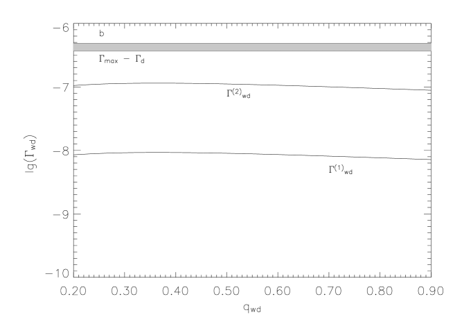
Figure 3: In panel a, the microlensing rate $\Gamma_{\rm wd}$ expected for the white dwarf disk model is shown as a function of the disk scale height $H_{\rm wd}$. The curve labelled $\Gamma^{(1)}_{\rm wd}$ corresponds to a local white dwarf mass density $\rho_{\rm wd}(R_{0})=1.3\times 10^{-4}~{}M_{\odot}$ pc^-3 while the band labelled $\Gamma^{(2)}_{\rm wd}$ corresponds to mass density values $\rho_{\rm wd}(R_{0})=3.4^{+0.5}_{-0.5}\times 10^{-3}~{}M_{\odot}$ pc^-3. In panel b white dwarfs are assumed to be distributed according to a spheroidal model with flatness parameter $q_{\rm wd}$. The curve labelled $\Gamma_{\rm wd}^{(1)}$ corresponds to the same white dwarf mass density as in panel a while the curve $\Gamma_{\rm wd}^{(2)}$ corresponds to $\rho_{\rm wd}(R_{0})=1.6\times 10^{-3}~{}M_{\odot}$ pc^-3 which follows from the constraints of the observed optical depth (see Fig. 1b and discussion in the text).

In Fig. 3 we present the obtained microlensing rates for white dwarfs models in the disk distribution (Fig. 3a) and in the spheroidal distribution (Fig. 3b). The curve labeled as $\Gamma^{(2)}_{\rm wd}$ in Fig. 3a is given for $\rho_{\rm wd}(R_{0})=3.4^{+0.5}_{-0.5}\times 10^{-3}~{}M_{\odot}$ pc^-3 while in Fig. 3b we have adopted only the upper limit for the white dwarf local density allowed by observations (see the discussion above). For comparison, we also give the differnce (grey band) between the maximum allowed rate $\Gamma_{\rm max}=(3.8-5)\times 10^{-7}$ yr^-1 (which corresponds to the 13-17 events detected so far in microlensing experiments towards the LMC, [5]) and that estimated for the standard stellar disk. To estimate $\Gamma_{\rm max}$ we have assumed a total number of observed LMC stars $N_{*}=1.19\times 10^{7}$ during an observation time of $t_{\rm obs}=5.7$ yr and adopted the instrument detection efficiency $\epsilon(t_{\rm E})$ given by the MACHO Collaboration. [33] Notice that we are neglecting the source spatial distribution. The only effect of this is that we are unable to estimate the expected event number as a function of the direction and the number of expected self-lensing events.

Once the microlensing rate for each lens population has been calculated, it is straightforward to obtain the expected number of microlensing events by eq. (15).

30pcThe expected number of events for different types of lenses and models are reported. For white dwarfs in the spheroidal models (first four lines) we assume $a_{\rm wd}=2~{}{\rm kpc}$. The assumed mass values are $m_{\rm d}=0.4~{}M_{\odot}$ for disk stars, $m_{\rm h}=0.5~{}M_{\odot}$ for halo lenses and $m_{\rm wd}=0.65~{}M_{\odot}$ for white dwarfs. We assume that about $20\%$ of the halo dark matter is made of MACHOs. The models labelled with $S$ correspond to white dwarfs distributed in spheroidal models with flatness parameter $q_{\rm wd}$ given as subscript. The models labelled as $D$ corresponds to white dwarfs distributed in disk models with height scale appearing as subscript (in kpc). The superscript $l$ corresponds to white dwarf local mass-density $\rho_{\rm wd}(R_{0})=1.3\times 10^{-4}~{}M_{\odot}$ pc^-3 while $h$ corresponds to $\rho_{\rm wd}(R_{0})=1.6\times 10^{-3}~{}M_{\odot}$ pc^-3 for spheroidal models and to $\rho_{\rm wd}(R_{0})=4.4\times 10^{-3}~{}M_{\odot}$ pc^-3 for disk models (for details see text). WD model $N_{\rm d}$ $N_{\rm h}$ $N_{\rm wd}$ $<t_{\rm d}>$ $<t_{\rm h}>$ $<t_{\rm wd}>$ $S_{0.2}^{l}$ $2.2$ $8.0$ $0.4$ $47\pm 18$ $50\pm 26$ $58\pm 25$ $S_{0.6}^{l}$ $2.2$ $8.0$ $0.4$ $47\pm 18$ $50\pm 26$ $66\pm 27$ $S_{0.2}^{h}$ $2.4$ $7.1$ $4.1$ $53\pm 21$ $50\pm 26$ $57\pm 24$ $S_{0.6}^{h}$ $2.4$ $7.1$ $4.4$ $53\pm 20$ $51\pm 26$ $66\pm 27$ $D_{3}^{l}$ $2.0$ $8.3$ $0.1$ $50\pm 20$ $31\pm 14$ $45\pm 14$ $D_{5}^{l}$ $2.0$ $8.4$ $0.1$ $50\pm 20$ $31\pm 14$ $42\pm 14$ $D_{1}^{h}$ $2.0$ $8.4$ $0.3$ $49\pm 19$ $31\pm 14$ $58\pm 22$ $D_{3}^{h}$ $2.0$ $8.4$ $1.2$ $49\pm 19$ $31\pm 14$ $42\pm 13$

The obtained results are given in Table 5 for some selected models. As one can see, the expected number of events for white dwarfs in the spheroidal model results in the range $0.4-4.4$, for the lower ($\rho_{\rm wd}(R_{0})=1.3\times 10^{-4}~{}M_{\odot}$ pc^-3 given by [22]) and upper ($\rho_{\rm wd}(R_{0})=4.4\times 10^{-3}~{}M_{\odot}$ pc^-3 taking two standard deviations for the local white dwarf mass density estimated by [20]) local mass density values, respectively. For white dwarfs in the disk model the expected number of events is $0.1-1.2$, for the lower and upper local mass density values, respectively. Clearly, if one considers that the total number of events observed by the MACHO Collaboration in a 5.7 years campaign towards the LMC is $13-17$ [5] and that 3-4 of these events are expected to be due to self-lensing [6], the obtained results may be considered as consistent with observations for all white dwarf models.

In principle, the mean time duration of the microlensing events caused by each of the three lens components could be a better indicator to investigate the presence of a white dwarf component through microlensing searches. In the same Table we give the mean event duration $<t_{\rm E}>$, with the relative uncertainty $\sigma_{<t_{\rm E}>}$, of microlensing events from stellar disk lenses, halo lenses and selected models of white dwarf distributions. To estimate $\sigma_{<t_{\rm E}>}$ we use a Montecarlo program to obtain the event duration distributions (which are given in Fig. 4) and we define $\sigma_{<t_{\rm E}>}$ so that $<t_{\rm E}>-\sigma_{<t_{\rm E}>}$, $<t_{\rm E}>+\sigma_{<t_{\rm E}>}$ is the duration range containing $50\%$ of expected events.

As one can see from the Table, it is extremely difficult to really distinguish between the different lens populations since they have comparable average duration values. This is also more clear in Fig. 4 in which the probability distribution (upper panels) and the distribution of the number of events (lower panels) for each galactic population are shown as a function of the microlensing duration for the fourth and eighth model given in the Table. The curves shown allow to directly estimate the probability that an observed event belong to one of the considered populations.

Figure 4: The differential event number ${\rm d}N_{\rm ev}(t_{\rm E})/{\rm d}t_{\rm E}$ (lower panels) is given as a function of the duration $t_{\rm E}$, for the fourth (right) and eighth (left) model in the Table. For each lens component, the curves are normalized to the respective total number of events quoted in the Table. In the upper panels, for the same models, the probability for each lens population is also given as a function of $t_{\rm E}$. As in the previous Figures, we adopt dotted, dashed and continuous lines for halo, disk and white dwarf lens components, respectively. We note that the fluctuations in the curves are due to the Montecarlo method.

6 Conclusions

In the present paper we have considered, in addition to the standard stellar disk, bulge and halo lens populations, gravitational microlensing towards the LMC also from a population of white dwarfs distributed according to two different models: thick disk and spheroidal shape with various flatness values.

By comparing optical depth theoretical results and observational data towards the LMC we find for the local mass density of white dwarfs in the spheroidal distribution an upper limit of about $\rho_{\rm wd}(R_{0})\simeq 1.6\times 10^{-3}~{}M_{\odot}$ pc^-3. For white dwarfs distributed according to disk models, instead, available observations are unable to set an upper limit on the white dwarf local mass density value.

We have then calculated the expected microlensing rate from each lens population model, the average event duration $<t_{\rm E}>_{\rm i}$ and the expected number of events $N_{\rm ev,i}$ for each galactic lens population by taking into account the detection efficiency given by the MACHO Collaboration. [33]

In the Table our main results for selected lens models are presented. As one can see, the expected number of events for white dwarfs in the spheroidal model results in the range $0.4-4.4$, for the lower and upper local mass density values, respectively. For white dwarfs in the disk model the expected number of events is $0.1-1.2$, for the lower and upper local mass density values. Clearly, if one considers that the total number of observed events is $13-17$ [5] and that $3-4$ events can be accounted for by self-lensing, [6] the obtained results may be considered as consistent with observations. The event durations for the various adopted models are given in the Table. From this Table and Fig. 4 it is clear how it is difficult to distinguish between the various lens populations, since the obtained distributions look similar. Therefore, microlensing observations alone cannot allow at present to understand the nature of the lens. Indeed, in order to distinguish among different lens populations, one should eliminate the degeneracy in microlensing observations (which give as a result the event duration and the source amplification) since a direct measurement of the MACHO distance, mass or transverse velocity is generally not possible. The best way to solve the issue is to perform parallax observations of microlensing events since it allows a direct measurement of the MACHO distance to the observer. [34, 35, 36] On the other hand, this requires telescopes in orbit around the Sun, which is probably rather far in the future.

In any case, present and future microlensing and pixel lensing observations towards different directions - e.g. M31 [37] or other nearby galaxies - should allow to increase the available statistics of microlensing events towards several directions getting, through an accurate data analysis, more information about the possible presence of different lens populations in the Galaxy. Moreover, it will be possible to find an increasing number of microlensing events for which parallax measurements (or a direct imaging of the lens through the next generation of space-based telescopes) may allow to solve the parameter degeneracy allowing a direct estimate of the lens mass and distance.

References

- [1] SAHU K. C., Nature 370 (1994) 275
- [2] SAHU K. C. and SAHU M. S., Astrophys. J. 508 (1998) L147
- [3] SALATI P. et al., Astron. Astrophys. 350 (1999) L57
- [4] GYUK G., DALAL N. and GRIEST K., Astrophys. J. 535 (2000) 90
- [5] ALCOCK C. et al., Astrophys. J. 542 (2000) 281
- [6] JETZER Ph., MANCINI L. and SCARPETTA G., Astron. Astrophys.393 (2002) 129
- [7] GIBSON B. and MOULD J. Astrophys. J. 482 (1997) 98
- [8] BINNEY J., MNRAS 307(1999) L27
- [9] De PAOLIS F., INGROSSO G., JETZER Ph. and RONCADELLI M. Mon. Not. R. Astron. Soc. 294 (1998) 283
- [10] DI STEFANO R., Astrophys. J. 541 (2000) 587
- [11] HANSEN B., Astrophys. J. 520 (1999) 680
- [12] LENZUNI P., CHERNOFF D. F. and SALPETER E. E. Astrophys. J. 393 (1992) 232
- [13] TAYLOR J., Astrophys. J. 497 (1998) L81
- [14] KERINS E. J. and EVANS N. W., Astrophys. J. 503 (1998) L75
- [15] BENNETT D. P. et al., American Astronomical Society, 195th AAS Meeting 31 (1999) 1422
- [16] QUINN J. L. et al., American Astronomical Society Meeting N. 195 (1999) 3708
- [17] HANSEN B.M.S., Nature 394 (1998) 860
- [18] HANSEN B.M.S., Astrophys. J. 558 (2001) L39
- [19] IBATA R. et al., Astrophys. J. 524 (1999) 95
- [20] HOLBERG J. B., OSWALT, T. D. and SION E. M., Astrophys. J. 571 (2002) 512
- [21] BAHCALL J.N., SCHMIDT M. and SONEIRA R.M., Astrophys. J. 265, (1983) 730
- [22] OPPENHEIMER B. R. et al., Science 292 (2001) 698
- [23] WOOD M.A. and OSWALD T.D., Astrophys. J. 497 (1998) 870
- [24] GOULD A., FLYNN C. and BAHCALL J. N., Astrophys. J. 503 (1998) 798
- [25] REID I. N., SAHU K. and HAWLEY S. L., preprint astro-ph/0104110 (2001)
- [26] REID I. N., HAWLEY S. L. and GIZIS J. E., Astronomical J. 110 (1995) 1838
- [27] DAVIES M. B., KING A. and RITTER H., Mon. Not. R. Astron. Soc. 333(2002) 463
- [28] BERGERON P. preprint astro-ph/0211569 (2002)
- [29] DWEK, E. et al. Astrophys. Journal 445 (1995) 716
- [30] GILMORE G., WYSE R.F.G. and KUIJKEN K., Ann. Rev. Astron. Astrophys. 27 (1989) 555
- [31] PACZYŃSKI B., Astrophys. J. 304, (1986) 1
- [32] GRIEST K. Astrophys. J. 366, (1991) 412
- [33] ALCOCK C. et al. Astrophys. Journal 136 (2001) 439
- [34] GAUDI B. S. and GOULD A., Astrophys. J. 477 (1997) 152
- [35] HAN C. and KIM H., Astrophys. J. 528 (2000) 687
- [36] SOSZKYŃSKI I. et al., Astrophys. J. 552 (2001) 731
- [37] CALCHI NOVATI S. et al., Astron. Astrophys. 381 (2002) 848