WMAP, neutrino degeneracy and non-Gaussianity constraints on isocurvature perturbations in the curvaton model of inflation

Abstract

In the curvaton model of inflation, where a second scalar field, the ‘curvaton’, is responsible for the observed inhomogeneity, a non-zero neutrino degeneracy may lead to a characteristic pattern of isocurvature perturbations in the neutrino, cold dark matter and baryon components. We find the current data can only place upper limits on the level of isocurvature perturbations. These can be translated into upper limits on the neutrino degeneracy parameter. In the case that lepton number is created before curvaton decay, we find that the limit on the neutrino degeneracy parameter is comparable with that obtained from Big-bang nucleosynthesis. For the case that lepton number is created by curvaton decay we find that the absolute value of the non-Gaussianity parameter,$|f_{\rm nl}|$, must be less than 10 (95% confidence interval).

I Introduction

In single field models of inflation, the inflaton gives rise to an era of accelerated expansion in the early universe during which quantum fluctuations in the inflaton field are expanded beyond the horizon size LLBook . At the end of inflation, the inflaton decays into the standard matter fields. The primordial fluctuations, imprinted onto the gravitational potential in form of small perturbations, become the “seeds” that start the formation of large scale structure. As there is only a single degree of freedom, the inflaton’s value, the resulting perturbations are always adiabatic, i.e. the ratio of the number densities of different particle species is spatially homogeneous, there is no isocurvature mode.

Recently a different model has been proposed, the curvaton scenario curvaton ; LUW , which has already received considerable attention allcurvaton ; MWU ; DHLDW ; gordonlewis . In this model the accelerated expansion is still provided by the inflaton, but the primordial perturbations are generated by another scalar field, the curvaton. The curvaton energy density is small compared to the inflaton energy density and being a light field, it acquires an almost scale-invariant spectrum of perturbations during inflation. After the decay of the inflaton, the isocurvature perturbation in the curvaton fluid is transformed into an adiabatic perturbation Mollerach ; LM ; MWU and the curvaton decays into radiation and other particles. A similar model to the curvaton scenario, in which a second scalar field determines the inflaton decay rate, has also been proposed recently vardecay .

The curvaton scenario requires different constraints on the inflationary potential to standard inflation and might therefore be better suited for inflation at a lower energy scale lythdimopolos ; lythsmallscale . It also allows for the possibility of an isocurvature mode in the standard matter fields curvaton ; LUW , i.e. the ratio of particle number densities of different particle species is not necessarily spatially homogeneous. This arises since the final constituents of the standard big bang model (photons, neutrinos, baryons and cold dark matter (CDM)) do not all necessarily originate entirely from the spatially inhomogeneous curvaton, but may originate instead from the spatially homogeneous inflaton or some other source.

In Ref. gordonlewis the isocurvature components in the CDM and baryons that could arise in the curvaton scenario were constrained using WMAP and other observational data. It was found that the current data rule out either CDM or baryons being created before curvaton decay. In this article we examine what the current observational constraints are on neutrino isocurvature perturbations created by curvaton decay. These can only arise if there is a non-zero neutrino degeneracy parameter $\xi=\mu_{\nu}/T_{\nu}$, where $\mu_{\nu}$ is the neutrino chemical potential and $T_{\nu}$ is the neutrino temperature LUW . There may be a separate degeneracy parameter for each of the three species of neutrinos, but the recent atmospheric and solar neutrino data indicate that approximate flavor equilibrium between all active neutrino species is established well before the BBN epoch solar and hence we take the degeneracy parameters to be equal.

Various studies have constrained the value of $\xi$ using CMB and other large scale structure data in the adiabatic case xibg . However, the tightest constraints still come from Big-bang nucleosynthesis (BBN) bbnxi . In this article we examine how the constraints on $\xi$ change in the curvaton scenario where neutrino isocurvature perturbations can be induced by a non-zero $\xi$. It turns out that the neutrino isocurvature perturbations then also induce baryon and CDM isocurvature perturbations LUW . It is therefore not possible to use constraints that have simply considered the addition of a neutrino isocurvature mode such as Ref. garcia-bellido or those that have considered arbitrary combinations of different isocurvature perturbations multiiso .

In the next section we evaluate the possible magnitudes of the neutrino isocurvature perturbations. Then in Sec. III we estimate analytically the effects of the isocurvature perturbations on the temperature fluctuations of the CMB and their dependence on $\xi$. A full likelihood analysis of the allowed ranges of $\xi$ is given in Sec. IV. Finally, the conclusions and the discussion are given in Sec. V.

II Curvaton generated neutrino isocurvature perturbations

A useful gauge-invariant variable for characterizing inhomogeneity on large scales is BST ; Bardeen88 ; WMLL

$$\zeta=-\psi-H\frac{\delta\rho}{\dot{\rho}}\,,$$ (1)

where $\rho$ and $H$ are respectively the total energy density and the Hubble parameter, the dot denotes differentiation with respect to coordinate time, and the perturbation in a background quantity $x$ is denoted by $\delta x$. For a critical density Universe, $\psi$ is related to the intrinsic curvature of a spatial hypersurface by WMLL

$${}^{(3)}R=\frac{4}{a^{2}}\nabla^{2}\psi\,,$$ (2)

where $a$ is the scale factor and $\nabla_{i}$ is the covariant derivative. It is possible to choose the coordinate system such that certain combinations of perturbation variables are set to zero. This is known as choosing the gauge or frame Bardeen ; KS ; WMLL . In this article we will work in the flat gauge Bardeen ; KS ; WMLL in which $\psi=0$, and Eq. (1) becomes

$$\zeta=-H\frac{\delta\rho}{\dot{\rho}}\,,$$ (3)

where from now on $\delta x$ refers to the perturbation in $x$ when the flat gauge is chosen. The energy conservation equation is given by

$$\dot{\rho}+3H(\rho+P)=0\,,$$ (4)

where $P$ is the total pressure. After curvaton ($\sigma$) decay, the component fluids are photons ($\gamma$), neutrinos $(\nu)$, cold dark matter (${\rm cdm}$) and baryons ($\mathrm{B}$). The total energy density and pressure are related to density and pressure of a component $i$ by $\rho=\sum_{i}\rho_{i}$ and $P=\sum_{i}P_{i}$. The component pressures are given in terms of the corresponding component densities: $P_{i}=\rho_{i}/3$ for photons and neutrinos and $P_{i}=0$ for the curvaton (after the end of inflation), CDM and baryons.

We assume a critical density Universe and that the neutrinos are effectively massless.

The isocurvature perturbations are given by MWU

$$\mbox{$\cal S$}_{i}=3(\zeta_{i}-\zeta_{\gamma})\,,$$ (5)

where $i$ is one of $\sigma$, $\nu$, ${\rm cdm}$ or $\mathrm{B}$ and

$$\zeta_{i}=-H\frac{\delta\rho_{i}}{\dot{\rho}_{i}}\,.$$ (6)

If there is no energy transfer to and from a fluid so that it satisfies the energy conservation equation:

$$\dot{\rho_{i}}+3H(\rho_{i}+P_{i})=0\,,$$ (7)

then its $\zeta_{i}$ is conserved on large scales, $\dot{\zeta_{i}}=0$ WMLL .

The occupation number for a neutrino species ($i=e$, $\mu$ or $\tau$) with energy $E$ is given by

$$f_{i}(E)=[\exp(E/T_{\nu}\mp\xi_{i})+1]^{-1}\,,$$ (8)

where $T_{\nu}$ is the neutrino temperature and the minus is for neutrinos and the plus for anti-neutrinos. The degeneracy parameter is $\xi_{i}=\mu_{i}/T_{\nu}$ where $\mu_{i}$ is the chemical potential of species $i$. However, using the Large Mixing Angle (LMA) solution leads to the degeneracy parameter being approximately the same for all three species solar , i.e. $\xi_{i}=\xi$. After positron annihilation, the asymmetry parameter, $\xi$, is constant in time LUW . When $\xi$ is non-zero, the difference between the number densities of neutrinos and anti-neutrinos is non-zero. We denote this quantity $n_{L}$ as this difference is equal to the lepton number. Given the constraints on charge asymmetry, any non-negligible lepton number must be due to the neutrinos. There can be no neutrino isocurvature perturbation when $n_{L}=0$ as then the neutrino energy density is determined solely by the photon energy density before neutrino decoupling LUW .

Analogously to the case of energy density, Eq. (6), the inhomogeneity of lepton number can be characterized by

$${\zeta}_{L}=-H\frac{\delta n_{L}}{\dot{n}_{L}}\,,$$ (9)

where as specified before we are using $\delta n_{L}$ in the flat gauge. If the lepton number density is conserved

$$\dot{n}_{L}+3Hn_{L}=0\,,$$ (10)

then $\dot{\zeta}_{L}=0$ on large scales LUW ; DHLDW .

The isocurvature perturbation of the lepton number perturbation is then given by

$${\mbox{$\cal S$}}_{\mathrm{L}}=3({\zeta}_{\mathrm{L}}-\zeta_{\gamma})\,,$$ (11)

which is related to the neutrino isocurvature perturbation by LUW

$$\mbox{$\cal S$}_{\nu}=\frac{45}{7}\frac{B^{2}}{B^{\prime}A}\mbox{$\cal S$}_{\mathrm{L}}\,,$$ (12)

where

$$A = \left[3.04/3+\frac{30}{7}\left(\frac{\xi}{\pi}\right)^{2}+\frac{15}{7}\left(\frac{\xi}{\pi}\right)^{4}\right]\,,$$ (13)

$$B = \left[\frac{\xi}{\pi}+\left(\frac{\xi}{\pi}\right)^{3}\right]\,,$$ (14)

and $B^{\prime}=1+3(\xi/\pi)^{2}$. The $3.04/3$ term in the definition of $A$ takes into account the non-equilibrium heating of the neutrino fluid and finite temperature QED corrections Dolgov ; bbnxi ; QED .

If the lepton number is created well before the curvaton decay then it will have negligible perturbations (${\zeta_{\mathrm{L}}}=0$) and so from Eq. (11)

$${\mbox{$\cal S$}}_{\mathrm{L}}=-3\zeta_{\gamma}\,.$$ (15)

We will not make the assumption $|\xi|\ll 1$, which was used in Ref. curvaton as we will be also considering the case where $\xi$ may be large. To evaluate the effect of $\mbox{$\cal S$}_{\nu}$ on observations we need to express it in terms of the adiabatic perturbation $\zeta$. To do this we can use Eqs. (3), (4) and (6) and that only the photons and neutrinos contribute significantly to the density in the primordial era to get

$$\zeta=(1-R_{\nu})\zeta_{\gamma}+R_{\nu}\zeta_{\nu}\,,$$ (16)

where

$$R_{\nu}=\frac{\rho_{\nu}}{\rho_{\nu}+\rho_{\gamma}}\,,$$ (17)

which can be evaluated using Dolgov ; bbnxi

$$\rho_{\nu}=\frac{7}{8}\left(\frac{4}{11}\right)^{4/3}3A\rho_{\gamma}\,.$$ (18)

Combining Eq. (16) with Eq. (5) for $i=\nu$ we get

$$\zeta=\zeta_{\gamma}+\frac{1}{3}R_{\nu}\mbox{$\cal S$}_{\nu}\,,$$ (19)

then solving Eq. (19) for $\zeta_{\gamma}$ and substituting into Eq. (15) gives

$$\mbox{$\cal S$}_{L}=-3\zeta+R_{\nu}\mbox{$\cal S$}_{\nu}.$$ (20)

Substituting Eq. (20) into Eq. (12) and solving for the neutrino isocurvature perturbation gives

$$\mbox{$\cal S$}_{\nu}=\frac{135B^{2}}{45B^{2}R_{\nu}-7B^{\prime}A}\zeta\,.$$ (21)

If the lepton number is created by curvaton decay then LUW

$${\zeta}_{L}=\zeta_{\sigma}=\frac{\zeta}{r}\,,$$ (22)

where using the sudden decay approximation, $r\approx\rho_{\sigma}/(\rho_{\sigma}+\rho_{\gamma})$ evaluated at the time of curvaton decay. The approximation is accurate up to about 10 % error even when the decay is not sudden MWU . Using Eq. (5) (with $i=\nu$), Eqs. (11), (16) and (22) gives

$$\mbox{$\cal S$}_{L}=3\frac{1-r}{r}\zeta+R_{\nu}\mbox{$\cal S$}_{\nu}\,.$$ (23)

Substituting Eq. (23) into Eq. (12) and solving for $\mbox{$\cal S$}_{\nu}$ we get

$$\mbox{$\cal S$}_{\nu}=\frac{r-1}{r}\frac{135B^{2}}{45B^{2}R_{\nu}-7B^{\prime}A}\zeta\,,$$ (24)

which is valid even when $\xi^{2}$ is large. As can be seen, the neutrino isocurvature perturbation resulting from lepton number created by curvaton decay, Eq. (24), differs from the neutrino isocurvature perturbation result when lepton number is created before curvaton decay, Eq. (21), by a factor which is only a function of $r$.

The final possibility is for the lepton number to be created after curvaton decay which corresponds to $r=1$ in Eq. (24) and so in this case there is no neutrino isocurvature perturbation.

If there is a neutrino isocurvature perturbation it induces a CDM and baryon isocurvature perturbation LUW . In the case where CDM or baryons are created after curvaton decay LUW :

$$\mbox{$\cal S$}_{{\rm cdm}/\mathrm{B}}=R_{\nu}\mbox{$\cal S$}_{\nu}\,,$$ (25)

where $\mbox{$\cal S$}_{{\rm cdm}/\mathrm{B}}$ stands for $\mbox{$\cal S$}_{{\rm cdm}}$ or $\mbox{$\cal S$}_{\mathrm{B}}$ as the effect is the same on either one. When CDM/B is created before curvaton decay there is an additional residual contribution LUW :

$$\mbox{$\cal S$}_{{\rm cdm}/\mathrm{B}}=R_{\nu}\mbox{$\cal S$}_{\nu}-3\zeta\,.$$ (26)

When CDM/B is created by curvaton decay

$$\mbox{$\cal S$}_{{\rm cdm}/\mathrm{B}}=R_{\nu}\mbox{$\cal S$}_{\nu}+3\frac{1-r}{r}\zeta\,.$$ (27)

However, to concentrate on the role of neutrino isocurvature perturbations we will only consider the case where baryon number and CDM are created after curvaton decay, Eq. (25).

III Neutrino Degeneracy Modifications of the Sachs-Wolfe effect

In this section we examine analytically the effect of a neutrino degeneracy in the curvaton scenario.

In the presence of isocurvature perturbations the temperature fluctuations due to the Sachs-Wolfe effect SW ; KSrad1 on large scales are given by gordonlewis

$$\frac{\Delta T}{T}=-\frac{1}{5}\zeta^{\text{rad}}-\frac{2}{5}\left(R_{\mathrm{B}}\mbox{$\cal S$}_{\mathrm{B}}+R_{\rm cdm}\mbox{$\cal S$}_{{\rm cdm}}\right)+\frac{1}{15}R_{\nu}\mbox{$\cal S$}_{\nu}\,,$$ (28)

where $\zeta^{\text{rad}}$ is the value of $\zeta$ in the radiation era and

$$R_{\mathrm{B}} = \frac{\rho_{\mathrm{B}}}{\rho_{\mathrm{B}}+\rho_{\rm cdm}},$$ (29)

$$R_{\rm cdm} = \frac{\rho_{\rm cdm}}{\rho_{\mathrm{B}}+\rho_{\rm cdm}}.$$ (30)

Substituting the induced baryon isocurvature perturbations Eq. (25) into Eq. (28) and making use of Eqs. (29) and (30) gives

$$\frac{\Delta T}{T}=-\frac{1}{5}\zeta^{\text{rad}}-\frac{1}{3}R_{\nu}\mbox{$\cal S$}_{\nu}.$$ (31)

The current 95% confidence interval (CI) limits on $\xi$ from BBN are bbnxi

$$-0.03\leq\xi\leq 0.11.$$ (32)

So in order to determine whether within these limits the isocurvature perturbations can still play a role we can use $\xi\ll 1$ which gives from Eqs. (14), (17) and (18) gives

$$R_{\nu}\approx 0.41.$$ (33)

Substituting Eq. (33) into Eq. (31) gives

$$\frac{\Delta T}{T}\approx-\frac{1}{5}\left(\zeta^{\text{rad}}+\frac{1}{2}\mbox{$\cal S$}_{\nu}\right)\,,$$ (34)

which shows that the neutrino isocurvature perturbation has a similar sized effect as the adiabatic perturbation on large scales.

For the lepton number created before curvaton decay with $\xi\ll 1$, Eq. (21) gives

$$\mbox{$\cal S$}_{\nu}\approx-\frac{135}{7}\left(\frac{\xi}{\pi}\right)^{2}\zeta$$ (35)

which when substituted into Eq. (34) results in

$$\frac{\Delta T}{T}\approx\frac{1}{5}\left(-1+\xi^{2}\right)\zeta^{\text{rad}}.$$ (36)

Hence in this case the neutrino degeneracy decreases the temperature fluctuations on large scales. However, for the BBN limits of $|\xi|\leq 0.11$ it follows from Eq. (36) that the isocurvature perturbation has a negligible effect on the temperature fluctuations when the lepton number is created before curvaton decay.

For lepton number created by curvaton decay with $\xi\ll 1$, Eq. (24) gives

$$\mbox{$\cal S$}_{\nu}=\frac{1-r}{r}\frac{135}{7}\left(\frac{\xi}{\pi}\right)^{2}\zeta.$$ (37)

¿From Eq. (37) and Eq. (34) we then find

$$\frac{\Delta T}{T}\approx\frac{1}{5}\left(-1+\frac{r-1}{r}\xi^{2}\right)\zeta^{\text{rad}}\,.$$ (38)

As can be seen from Eq. (38), in the case where the lepton number is created by curvaton decay, a non-zero $\xi$ adds to the magnitude of the fluctuations on large scales as $0\leq r\leq 1$. Limits on $r$ can be placed using the limits on the non-Gaussianity parameter $f_{\rm nl}$ LUW ; curvatonfnl

$$f_{\rm nl}=\frac{1}{3}+\frac{5}{6}r-\frac{5}{4r}\,.$$ (39)

The current WMAP limits two sigma confidence interval is Komatsu

$$-58\leq f_{\rm nl}\leq 134\,.$$ (40)

Inverting Eq. (39) this leads to $r\geq 0.02$ at two sigma confidence level. So from Eq. (38), it appears that there may be scope for a large contribution by the isocurvature term. We will test this with a full likelihood approach in the next Section.

IV Data Analysis

The effect of a non-zero $\xi$ on all cosmological scales can be obtained by inputting the isocurvature perturbations derived in Eqs. (21) and (24) and the induced baryon and CDM isocurvature perturbations, Eq. (25), into CAMB. To account for the effect on the background dynamics the number of massless neutrinos needs to be set to

$$N_{\nu}=3A$$ (41)

where $A$ is defined in Eq. (14). Some example cases are plotted in Fig. 1.

Figure 1: An illustration of the effect of the lepton degeneracy ($\xi$) on the spectrum of fluctuations. The cosmological parameters (including the amplitude) for all the spectra are taken from the maximum likelihood when $\xi=0$. The solid line is a plot of the pure adiabatic spectrum. The short dashed line is for the case when the lepton number is created before curvaton decay and $\xi=0.3$. The long dashed line is for the case when the lepton number is created by curvaton decay with $\xi=0.3$ and the fraction of the density made up by the curvaton at curvaton decay ($r$) is set to 0.5. The dotted line is the spectrum for when the lepton number is created after curvaton decay (so that there are no isocurvature modes) and $\xi=1$. The binned WMAP TT data is also plotted.

This figure confirms the direction of the effect evaluated analytically on large scales in Eqs. (36) and (38), i.e. a non-zero $\xi$ decreases the power on large scales when the lepton number is created before curvaton decay and increases it when the lepton number is created by curvaton decay. As can be see from Fig. 1, there is a similar effect on the extrema of the acoustic peaks but not on the rise and fall of the acoustic peaks. There is also a slight shift in the phase of the oscillations. As can also be seen in Fig. 1, a similar effect of a non-zero $\xi$ occurs when there are no isocurvature modes xibg ; bashinskyseljak but then there is no effect on the Sachs-Wolfe plateau. Note that the decrease or increase is fairly constant over large scales and so is not suitable for resolving the quadrupole problem quad .

The current BBN constraints on $\xi$ are given in Eq. (32). They rely on using the large angle solution in which all the $\xi$ for the three neutrino species become equal solar . The actual constraint is on $\xi_{e}$, the electron neutrino degeneracy, due to its effect on the neutron to proton ratio prior to BBN. There have been attempts to check the BBN constraint by independently using CMB and other large scale structure data xibg . This has been done in the context of adiabatic perturbations and so the effect is due to the increase of density caused by an greater effective number of neutrinos, Eq. (41).

In this Section we test what the constraints are when lepton number is created before and by curvaton decay. The adiabatic case is equivalent to when lepton number is created after curvaton decay as it corresponds to setting $r=1$ in Eq. (24). A modified version of COSMOMC cosmomc was used for the likelihood analysis which included WMAP temperature and temperature-polarization cross-correlation anisotropy WMAP , ACBAR ACBAR , CBI CBI , 2dF galaxy redshift survey 2dF and Hubble Space Telescope (HST) Key Project HST data. The Universe was taken as flat and the neutrinos as massless. Reionization was parameterized using optical depth Kosowsky . Each simulation used five separate Markov chains and the convergence criteria was taken to be the variance of the chain mean divided by the mean of the chain variance to be less than 0.2 for each parameter.

As COSMOMC produces Monte Carlo samples of the output variables, marginalization simply entails extracting the samples of the variables of interest from the multi-dimensional samples. These samples can then be used to evaluate confidence intervals or to give estimates of the probability distribution by using histograms. Functions of the variables can also be analyzed just by taking functions of the corresponding samples.

The different scenarios that were checked were: lepton number created before curvaton decay, Eq. (21), lepton number created by curvaton decay, Eq. (24), and lepton number created after curvaton decay. COSMOMC was modified to take extra variables $\xi$ and $r$ and their effect on the isocurvature modes, Eqs. (21), (24) and (25), and effective number of neutrinos, Eq. (41), were also added. Modifications were also made to allow the inclusion of a BBN prior on $\xi$ which is a Gaussian distribution with mean 0.04 and standard deviation $0.035$ bbnxi . The prior for $f_{\rm nl}$ was a Gaussian distribution with a mean of 38 and standard deviation of 48 Komatsu . This then imposed a prior on $r$ through Eq. (39).

In the cases where the BBN constraint was not used, only positive values of $\xi$ were sampled as then the results were even in $\xi$ as Eqs. (21), (24) and (41) are even in $\xi$.

The constraints on $\xi$ for the various possibilities considered are given in Table 1. The marginalized distributions for $\xi$ are also plotted in Fig. 2.

The BBN constraint is still tighter than that obtained by using the CMB, 2dF and HST data on any of the curvaton scenarios.

The case where lepton number is created before curvaton decay is only twice as broad without the BBN constraint. Also, in this case, the isocurvature contribution is almost 10% as large as the adiabatic contribution but this gets dramatically reduced when the BBN constraint is added.

The case when the lepton number is created by curvaton decay is less constraining on $\xi$ even though the data do allow about as much positive isocurvature perturbations as negative. This is because there is an additional degeneracy with $r$ as seen in Eq. (24) and so also in the two dimensional marginalized distribution of $\xi$ and $r$ as seen in Fig. 3. Adding the BBN constraint also dramatically decreases the amount of isocurvature perturbations in this case as the smaller values of $r$ needed to compensate for the lower $\xi$ is disfavored by the WMAP non-Gaussianity constraints on $f_{\rm nl}$. However, smaller values of $r$ are more likely with the BBN constraint and these lead to values of $f_{\rm nl}$ large enough in magnitude to possibly be detectable by the Planck satellite which may be sensitive to $|f_{\rm nl}|>5$ planck .

In the case where lepton number is created after curvaton decay, the constraints on $\xi$ are the broadest. In this case there are no isocurvature perturbations and a non-zero $\xi$ only effects the background dynamics through modifying the effective neutrino number, Eq. (41). This case has been studied before with similar results xibg .

Constraint	$\xi$	$\mbox{$\cal S$}_{\nu}/\zeta^{\text{rad}}$	$f_{\rm nl}$
BBN only	0.1
before curvaton decay	0.2	-0.08
BBN + before curvaton decay	0.1	-0.02
by curvaton decay	0.8	0.07	-4
BBN + by curvaton decay	0.1	0.04	-10
after curvaton decay	1.6

Table 1: Upper bound (95% CI) constraints on the magnitudes of the lepton degeneracy ($\xi$), the neutrino isocurvature perturbation ($\mbox{$\cal S$}_{\nu}$) and the non-Gaussianity parameter $f_{\rm nl}$. The ‘BBN’ label means the constraint from BBN using the large mixing angle solution bbnxi is included. The constraints from WMAP, ACBAR, CBI, 2dF and HST on the various curvaton mechanisms of generating the lepton number are given.

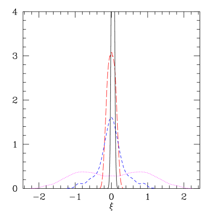
Figure 2: Comparison of marginalized probability distributions, using CMB, 2dF and HST data, for lepton degeneracy ($\xi$) when lepton number is created by curvaton decay (short-dashes), for lepton number created after curvaton decay (dotted) and for lepton number created before curvaton decay (long dashes). The BBN constraint on $\xi$ is also plotted (solid line).

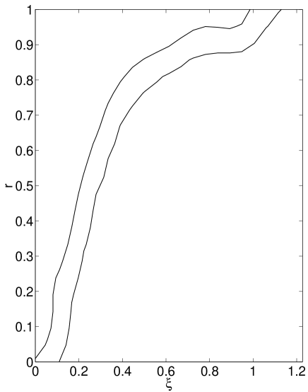
Figure 3: One and two sigma contours for the 2D marginalized probability distribution, using CMB, 2dF and HST data, of the lepton degeneracy ($\xi$) and the curvaton density proportion at time of curvaton decay ($r$) for the case when lepton number is created by curvaton decay.

V Conclusions

We have examined the current cosmological constraints on the neutrino degeneracy $\xi$, in the curvaton scenario, using WMAP, ACBAR, CBI, 2dF, HST and BBN data. The expressions for the isocurvature perturbations were evaluated to all orders in $\xi$ and the effects of the induced baryon and CDM isocurvature perturbations were accounted for. Analytical formulas were given for the modification of the Sachs-Wolfe effect on large scales.

Comparisons were made with the BBN constraint which results from the effect of the neutrino degeneracy on the pre-BBN proton to neutron ratio and using the large mixing angle solution in which the neutrino degeneracies of the different species take on the same value. It was found that the constraint on $\xi$ was comparable to that from BBN when the lepton number was created before curvaton decay. As seen in Fig. 1, a non-zero $\xi$ affects the acoustic peaks whose data will dramatically improve in the future. So the CMB constraints on $\xi$ may also improve dramatically. Without the BBN constraint, the neutrino isocurvature perturbation was found to be smaller than 10% the size of the adiabatic mode (95% CI), while including the BBN constraint reduced this by a factor of a few. In the case where the lepton number is created by curvaton decay, there is a degeneracy between the value of the curvaton energy density at the time of curvaton decay and $\xi$. However, this does not stop the BBN data strengthening the constraint on the isocurvature perturbation as the value of the curvaton energy density at the time of curvaton decay is constrained by the limits on the non-Gaussianity parameter from WMAP. So in this case, the neutrino isocurvature mode is less than about 5% (95% CI) of the adiabatic mode. Unless the BBN constraints on $\xi$ become tighter around zero, the case of the lepton number being created by curvaton decay would be unlikely if future observations found $f_{\rm nl}<-10$, as this would imply a larger isocurvature perturbation than is observed.

- (1) A. R. Liddle and D. H. Lyth, “Cosmological Inflation And Large-Scale Structure,” Cambridge, UK: Univ. Pr. (2000) 400 p.
- (2) D. H. Lyth and D. Wands, Phys. Lett. B 524, 5 (2002) [arXiv:hep-ph/0110002].
- (3) D. H. Lyth, C. Ungarelli and D. Wands, Phys. Rev. D 67, 023503-1-13 (2003) [arXiv:astro-ph/0208055].
- (4) T. Moroi and T. Takahashi, Phys. Lett. B 522, 215 (2001) [Erratum-ibid. B 539, 303 (2002)] [arXiv:hep-ph/0110096]; K. Enqvist and M. S. Sloth, Nucl. Phys. B 626, 395 (2002) [arXiv:hep-ph/0109214]; Phys. Rev. D 66, 063501 (2002) [arXiv:hep-ph/0206026]; K. Enqvist, S. Kasuya and A. Mazumdar, Phys. Rev. Lett. 90, 091302 (2003) [arXiv:hep-ph/0211147]; N. Bartolo and A. R. Liddle, Phys. Rev. D 65 (2002) 121301 [arXiv:astro-ph/0203076]. T. Moroi and T. Takahashi, Phys. Rev. D 66 (2002) 063501 [arXiv:hep-ph/0206026]. M. Fujii and T. Yanagida, Phys. Rev. D 66 (2002) 123515 [arXiv:hep-ph/0207339]. M. S. Sloth, Nucl. Phys. B 656 (2003) 239 [arXiv:hep-ph/0208241]. A. Hebecker, J. March-Russell and T. Yanagida, Phys. Lett. B 552 (2003) 229 [arXiv:hep-ph/0208249]. R. Hofmann, arXiv:hep-ph/0208267. T. Moroi and H. Murayama, Phys. Lett. B 553 (2003) 126 [arXiv:hep-ph/0211019]. K. Dimopoulos, G. Lazarides, D. Lyth and R. Ruiz de Austri, arXiv:hep-ph/0308015. K. Dimopoulos, D. H. Lyth, A. Notari and A. Riotto, JHEP 0307 (2003) 053 [arXiv:hep-ph/0304050]. K. Dimopoulos, G. Lazarides, D. Lyth and R. Ruiz de Austri, JHEP 0305 (2003) 057 [arXiv:hep-ph/0303154]. K. Dimopoulos, arXiv:astro-ph/0212264. M. Axenides and K. Dimopoulos, arXiv:hep-ph/0310194. K. Enqvist, A. Jokinen, S. Kasuya and A. Mazumdar, arXiv:hep-ph/0303165. M. Postma, Phys. Rev. D 67 (2003) 063518 [arXiv:hep-ph/0212005]. M. Postma, arXiv:astro-ph/0305101. A. R. Liddle and L. A. Urena-Lopez, Phys. Rev. D 68 (2003) 043517 [arXiv:astro-ph/0302054]. B. Feng and M. z. Li, Phys. Lett. B 564 (2003) 169 [arXiv:hep-ph/0212213]. J. McDonald, arXiv:hep-ph/0308295. J. McDonald, Phys. Rev. D 68 (2003) 043505 [arXiv:hep-ph/0302222]. M. Postma and A. Mazumdar, arXiv:hep-ph/0304246. S. Kasuya, M. Kawasaki and F. Takahashi, arXiv:hep-ph/0305134. K. Hamaguchi, M. Kawasaki, T. Moroi and F. Takahashi, arXiv:hep-ph/0308174. D. H. Lyth and D. Wands, arXiv:astro-ph/0306500. M. Bastero-Gil, V. Di Clemente and S. F. King, Phys. Rev. D 67, 103516 (2003) [arXiv:hep-ph/0211011]. M. Endo, M. Kawasaki and T. Moroi, Phys. Lett. B 569, 73 (2003) [arXiv:hep-ph/0304126]. M. Giovannini, arXiv:hep-ph/0310024.
- (5) K. A. Malik, D. Wands and C. Ungarelli, Phys. Rev. D 67 (2003) 063516 [arXiv:astro-ph/0211602].
- (6) D. H. Lyth and D. Wands, arXiv:astro-ph/0306498.
- (7) C. Gordon and A. Lewis, Phys. Rev. D 67 (2003) 123513 [arXiv:astro-ph/0212248].
- (8) S. Mollerach, Phys. Rev. D 42 (1990) 313.
- (9) A. D. Linde and V. Mukhanov, Phys. Rev. D 56, 535 (1997) [arXiv:astro-ph/9610219].
- (10) G. Dvali, A. Gruzinov and M. Zaldarriaga, arXiv:astro-ph/0305548; L. Kofman, arXiv:astro-ph/0303614; K. Enqvist, A. Mazumdar and M. Postma, Phys. Rev. D 67, 121303 (2003) [arXiv:astro-ph/0304187]; G. Dvali and S. Kachru, arXiv:hep-th/0309095;M. Axenides and K. Dimopoulos, arXiv:hep-ph/0310194;A. Mazumdar, arXiv:hep-th/0310162;G. Dvali and S. Kachru, arXiv:hep-ph/0310244; S. Tsujikawa, Phys. Rev. D 68, 083510 (2003) [arXiv:astro-ph/0305569]; C. Armendariz-Picon, astro-ph/0310512.
- (11) K. Dimopoulos and D. H. Lyth, arXiv:hep-ph/0209180.
- (12) D. H. Lyth, arXiv:hep-th/0308110.
- (13) S. Hannestad, Phys. Rev. D 65, 083006 (2002) [arXiv:astro-ph/0111423], A. D. Dolgov, S. H. Hansen, S. Pastor, S. T. Petcov, G. G. Raffelt and D. V. Semikoz, Nucl. Phys. B 632, 363 (2002) [arXiv:hep-ph/0201287]. Y. Y. Wong, Phys. Rev. D 66, 025015 (2002) [arXiv:hep-ph/0203180]. K. N. Abazajian, J. F. Beacom and N. F. Bell, Phys. Rev. D 66, 013008 (2002) [arXiv:astro-ph/0203442].
- (14) P. Crotty, J. Lesgourgues and S. Pastor, Phys. Rev. D 67, 123005 (2003) [arXiv:astro-ph/0302337]. E. Pierpaoli, Mon. Not. Roy. Astron. Soc. 342, L63 (2003) [arXiv:astro-ph/0302465]. S. Hannestad, JCAP 0305, 004 (2003) [arXiv:astro-ph/0303076].
- (15) A. Cuoco, F. Iocco, G. Mangano, G. Miele, O. Pisanti and P. D. Serpico, arXiv:astro-ph/0307213.
- (16) P. Crotty, J. Garcia-Bellido, J. Lesgourgues and A. Riazuelo, arXiv:astro-ph/0306286.
- (17) M. Bucher, K. Moodley and N. Turok, Phys. Rev. D 66, 023528 (2002) [arXiv:astro-ph/0007360]. M. Bucher, K. Moodley and N. Turok, Phys. Rev. Lett. 87, 191301 (2001) [arXiv:astro-ph/0012141]. R. Trotta, A. Riazuelo and R. Durrer, Phys. Rev. D 67, 063520 (2003) [arXiv:astro-ph/0211600].
- (18) J. M. Bardeen, P. J. Steinhardt and M. S. Turner, Phys. Rev. D 28, 679 (1983).
- (19) J. M. Bardeen, DOE/ER/40423-01-C8 Lectures given at 2nd Guo Shou-jing Summer School on Particle Physics and Cosmology, Nanjing, China, Jul 1988.
- (20) D. Wands, K. A. Malik, D. H. Lyth and A. R. Liddle, Phys. Rev. D 62 (2000) 043527 [astro-ph/0003278].
- (21) J. M. Bardeen, Phys. Rev. D 22 (1980) 1882.
- (22) H. Kodama and M. Sasaki, Prog. Theor. Phys. Suppl. 78 (1984) 1.
- (23) A. D. Dolgov, Phys. Rept. 370 (2002) 333 [arXiv:hep-ph/0202122].
- (24) D. A. Dicus et al. Phys.Rev. D26 (1982) 2694; S. Dodelson and M. S. Turner Phys.Rev. D46 (1992) 3372; S. Hannestad and J. Madsen Phys.Rev.D52:1764-1769,1995.
- (25) R. K. Sachs and A. M. Wolfe, Astrophys. J. 147 (1967) 73.
- (26) H. Kodama and M. Sasaki, Int. J. Mod. Phys. A 1 (1986) 265.
- (27) N. Bartolo, S. Matarrese and A. Riotto, arXiv:astro-ph/0309692.
- (28) E. Komatsu et al., Astrophys. J. Suppl. 148, 119 (2003) [arXiv:astro-ph/0302223].
- (29) S. Bashinsky and U. Seljak, arXiv:astro-ph/0310198.
- (30) D. N. Spergel et al., Astrophys. J. Suppl. 148, 175 (2003) [arXiv:astro-ph/0302209].
- (31) A. Lewis and S. Bridle, Phys. Rev. D 66, 103511 (2002) [arXiv:astro-ph/0205436]; A. Lewis, A. Challinor and A. Lasenby, Astrophys. J. 538, 473 (2000) [arXiv:astro-ph/9911177]; U. Seljak and M. Zaldarriaga, Astrophys. J. 469, 437 (1996) [arXiv:astro-ph/9603033].
- (32) G. Hinshaw et al., Astrophys. J. Suppl. 148, 135 (2003) [arXiv:astro-ph/0302217]; L. Verde et al., Astrophys. J. Suppl. 148, 195 (2003) [arXiv:astro-ph/0302218]; A. Kogut et al., Astrophys. J. Suppl. 148, 161 (2003) [arXiv:astro-ph/0302213].
- (33) C. l. Kuo et al. [ACBAR collaboration], arXiv:astro-ph/0212289.
- (34) T. J. Pearson et al., Astrophys. J. 591, 556 (2003) [arXiv:astro-ph/0205388].
- (35) W. J. Percival et al. [The 2dFGRS Team Collaboration], Mon. Not. Roy. Astron. Soc. 337 (2002) 1068 [arXiv:astro-ph/0206256].
- (36) W. L. Freedman et al., Astrophys. J. 553, 47 (2001) [arXiv:astro-ph/0012376].
- (37) A. Kosowsky, M. Milosavljevic and R. Jimenez, Phys. Rev. D 66, 063007 (2002) [arXiv:astro-ph/0206014].
- (38) E. Komatsu and D. N. Spergel, Phys. Rev. D 63, 063002 (2001) [arXiv:astro-ph/0005036].