The H$\alpha$ Galaxy Survey

We discuss the selection and observations of a large sample of nearby galaxies, which we are using to quantify the star formation activity in the local Universe. The sample consists of 334 galaxies across all Hubble types from S0/a to Im and with recession velocities of between 0 and 3000 km s^-1. The basic data for each galaxy are narrow band H$\alpha+$[Nii] and $R$-band imaging, from which we derive star formation rates, H$\alpha+$[Nii] equivalent widths and surface brightnesses, and $R$-band total magnitudes. A strong correlation is found between total star formation rate and Hubble type, with the strongest star formation in isolated galaxies occurring in Sc and Sbc types. More surprisingly, no significant trend is found between H$\alpha+$[Nii] equivalent width and galaxy $R$-band luminosity. More detailed analyses of the data set presented here will be described in subsequent papers.

1 Introduction

Knowledge of the star formation histories of both the Universe and of individual galaxies provides the foundation for our understanding of the evolution of the Universe we see today. Substantial advances have been made in our understanding of high-redshift star formation, (e.g. Madau et al. madau96 (1996); Madau et al. madau98 (1998); Steidel et al. stei (1999); Hopkins et al. hopk (2000); Lanzetta et al. lanz (2002)). This has resulted in an anomalous situation in which the star formation history of the Universe appears to be more fully quantified at high redshift than it is locally. This results at least partly from the relative ease with which a representative volume of the Universe can be observed at high redshift, since only a small area of the sky need be observed. Star formation rates have been determined for many local galaxies using a range of different techniques, e.g. emission-line fluxes (e.g., Kennicutt & Kent ken83 (1983); Young et al. young (1996); Gallego et al. gallego95 (1995); Gallego et al. gallego96 (1996)), far-infrared luminosities (e.g., Kennicutt et al. ken87 (1987)), radio luminosities (e.g., Condon condon (1992), Cram et al. cram (1998)) or direct ultraviolet emission from hot stars (e.g. Bell & Kennicutt bell (2001)). However, in the main these studies have looked at the brightest and most rapidly star-forming galaxies, and most spectroscopic studies are biased towards galaxies with large equivalent width (EW) in the line concerned. In this study, one focus will be on the star formation properties across the full range of the numerically dominant dwarf galaxies, and the global star formation rate from this population. A further consequence of the observational limitations on areal coverage is that galaxy clusters are easier to study than the field environment, and hence local field galaxy star formation rates are relatively poorly constrained compared with their cluster counterparts.

In the present study, we attempt to quantify star formation activity across the full range of star-forming galaxies, down to the faintest dwarf irregular types, by using narrow-band imaging through filters centred on the redshifted Balmer H$\alpha$ line. The advantages of this technique are that it is sensitive to low levels of star formation even in faint, low surface brightness galaxies, and that it traces high mass stars, and hence recent star formation. Given suitable assumptions, principally about extinction and the stellar initial mass function (IMF), it yields quantitative measurements of the star formation rate. The method can be applied to a sensitive level using relatively modest integration times on small telescopes, which is an important consideration given that this project must be done one object at a time, to ensure that each target galaxy is observed with the correct filter. The resulting data not only give estimates of the total star formation rate for each galaxy, but also detailed information on the star formation distribution, enabling, for example, the separation of nuclear and disk activity in spiral galaxies. Finally, the large format of current CCDs gives a reasonable probability of detecting nearby star-forming companion galaxies which lie in the same field as target galaxies, and which have similar recession velocities.

The principal drawbacks of narrow-band H$\alpha$ imaging are the need for large and uncertain extinction corrections; the need to assume an IMF to extrapolate from the quantity of high mass stars, responsible for the ionising flux, to the total mass of the young stellar population; contamination in most of the filters used by the [Nii] 6548 and 6584 Å lines, necessitating a further correction to the derived star formation rates; and possible contributions to the line emission by central active galactic nuclei (AGN). All of these assumptions and corrections have been investigated in detail, principally by Kennicutt and his collaborators (Kennicutt & Kent ken83 (1983); Kennicutt ken98 (1998)); we will re-examine some of the corrections they derived in Paper II of this series (James et al. jame (2003)). The final disadvantage of using narrow-band filters is that a comprehensive survey of a contiguous area (c.f. Sloan, IRAS) cannot be completed in a reasonable amount of time, due to the small recession velocity coverage of each of the narrow-band filters, and hence a pre-existing galaxy catalogue must be used to provide a target list for specific pointed observations with the appropriate filters.

Any discussion of previous work in this area must first acknowledge the extensive studies undertaken by Kennicutt and collaborators in defining the techniques for H$\alpha$ measurement and deriving star formation rates from such measurements (Kennicutt & Kent ken83 (1983)), and in applying these measurements to studies of bright spiral and irregular galaxies (e.g., Kennicutt et al. ken94 (1994)) and interacting galaxies (Kennicutt et al. ken87 (1987)). All of this work was comprehensively reviewed by Kennicutt (ken98 (1998)). Ryder & Dopita made a detailed study of 34 nearby southern spirals in H$\alpha$, $V$ and $I$ band emission, demonstrating that star formation can be much more asymmetric than the underlying stellar distribution (Ryder & Dopita ryde93 (1993)) and that the H$\alpha$ scale length tends to be longer than that of the stellar light distribution (Ryder & Dopita ryde94 (1994)). These observations were used to derive a form for the star formation law in spiral galaxies (Dopita & Ryder dopi94 (1994)). Young et al. (young (1996)) undertook a major study of 120 spiral galaxies using similar techniques to those used in the present work, to look at trends in H$\alpha$ surface brightness with Hubble type and at the dependence of star formation rate on gas mass and interactions. Koopman et al. (koopman (2001)) looked at the H$\alpha$ total emission and light profiles for 63 bright spiral galaxies in the Virgo cluster, again using narrow-band imaging techniques.

The Universidad Complutense de Madrid (UCM) emission-line survey (Gallego et al. gallego95 (1995), Gallego et al. gallego96 (1996)) adopted a different and in many ways complementary strategy of searching areas of sky for all emission-line galaxies over a wide range of recession velocities, using the objective prism technique to detect candidates, and follow-up spectroscopy for confirmation and derivation of detailed spectroscopic parameters. Gallego et al. (gallego96 (1996)) present H$\alpha$ and H$\beta$ fluxes and EWs for over 200 galaxies detected in this way, and Gallego et al. (gallego95 (1995)) use this dataset to determine the total star formation rate in the Local Universe. One of the aims of the present study is to rederive this parameter using a sample with very different selection criteria which are not dependent on H$\alpha$ line strengths. This will be presented in a later paper in this series. Finally, an important recent study with which the current work should be compared is that of Charlot and collaborators (e.g. Charlot et al. char02 (2002)), who used spectroscopic data from the Stromlo-APM survey to study a representative sample of star-forming galaxies with H$\alpha$ EW down to 0.2 nm, compared with a limit of 1.0 nm for Gallego et al. (gallego95 (1995)). The corresponding limit for the current survey is about 0.4 nm EW, although a few detections of line emission below this level are made.

The sample selection for the H$\alpha$ Galaxy Survey is described in Sect. 2 of this paper. The observational strategy and the data reduction process are detailed in Sections 3 and 4 respectively. Sect. 5 contains the data for the 334 galaxies, and Sect. 6 a discussion of some of the first results of this study. Sect. 7 contains our conclusions and a summary of planned future publications.

2 Sample selection

The sample was selected using the Uppsala Galaxy Catalogue (Nilson nilson (1973), henceforth UGC) as the parent catalogue. The UGC was chosen because of the uniform selection criteria used for its compilation (all galaxies to a limiting diameter of 1$\aas@@fstack{\prime}$0 and/or to a limiting apparent magnitude of 14.5 on the blue prints of the Palomar Observatory Sky Survey), its uniform coverage of the entire northern sky, its inclusion of galaxies of all Hubble types (including faint and low-surface-brightness dwarfs), and because it provides consistent diameters and classifications. The principal drawback of the UGC is that it does not contain recession velocities for many galaxies. This deficiency has largely been filled by studies since the publication of the UGC, and a search using the NASA Extragalactic Database (NED) shows that at least 85% of all UGC galaxies now have measured recession velocities. However, the remaining 15% cannot be selected for observation in our study, and this represents a possible source of bias which should be kept in mind when interpreting the results.

UGC galaxies were selected, using the NED ‘Advanced All-Sky Search For Objects By Parameters’ facility, within 5 recession velocity shells: 0–1000 km s^-1, 1000–1500 km s^-1, 1500–2000 km s^-1, 2000–2500 km s^-1, and 2500–3000 km s^-1. The galaxies were required to be spiral or irregular galaxies, with Hubble types from S0/a to Im inclusive, and to have $D_{25}$ diameters of 1$\aas@@fstack{\prime}$7–6$\aas@@fstack{\prime}$0. This last criterion ensures that all galaxies will fit on the field of the CCD camera used, and the different shells effectively sample different parts of the galaxy diameter function. Thus the central shell is dominated by dwarf Im and Sm galaxies, whilst the outer shells sample the rarer S0/a-Sc galaxies. The well-defined selection criteria, and the large total number of galaxies observed (334), mean that it is possible to combine the data for all shells such that galaxies with a wide range of luminosities, diameters and surface brightnesses are represented.

3 Observations

The primary data for this study are narrow-band H$\alpha+$[Nii] and Johnson $R$ band imaging. These observations were made using the 1.0 metre Jacobus Kapteyn Telescope (JKT), operated by the Isaac Newton Group of Telescopes (ING) situated on La Palma in the Canary Islands. This project was allocated 100 nights of observing time on the JKT, between February 2000 and January 2002. Of these nights, 78 produced usable data for the project and 52 were photometric. The instrument used was the facility 2048$\times$2048 pixel SITe CCD camera, with 0$\aas@@fstack{\prime\prime}$33 pixels, giving a total field of view of over 11^′$\times$11^′, of which the central area of 10^′$\times$10^′ is unvignetted. The CCD has a good quantum efficiency ($>$60%) in the $R$ band, and a read noise of about 7 electrons.

The filters used for this project are listed in Table 1. The relative throughputs are given, normalised to the $R$-band filter. The redshifted H$\alpha$ filters and the Harris $R$ filter are from the standard ING filter set, whereas the H$\alpha$Cont filter is an off-the-shelf item purchased for this project. The benefit of using this filter is that it accurately samples the galaxy continuum flux close to the H$\alpha$ line, but has a broader bandpass than the narrow H$\alpha$ filters, thus reducing the time overhead in taking continuum observations compared with using ‘off-line’ narrow H$\alpha$ filters. The H$\alpha$Cont filter proved useful in bright sky conditions (moonlight or dark twilight), but for fully dark skies it was found that scaled $R$-band exposures gave excellent continuum subtraction. The much greater speed of using the broad $R$ filter more than offsets the small loss in effective throughput to H$\alpha$ light that results from having the H$\alpha$ line within the passband of the $R$ filter. Standard exposure times used were 3$\times$1200 seconds in the appropriate narrow band filter, chosen to maximise throughput at the wavelength of the redshifted H$\alpha$ line; 300 seconds at $R$; and 3$\times$600 seconds in the H$\alpha$Cont filter if the $R$ image was not obtained in fully dark sky conditions. Additional calibrating $R$-band exposures were taken during a photometric night if there were any doubts about the sky conditions for the original observations. The very narrow [Nii] filter centred on 6584 Å was not used for general survey observations, but was useful for isolating just the H$\alpha$ line, and excluding [Nii] emission, for galaxies with recession velocities of approximately 1000 km s^-1. Such images will be used in a later paper for an examination of the effects of [Nii] contamination in our H$\alpha$ imaging, but are not used in the present paper. Hence all line fluxes presented here are for H$\alpha+$[Nii].

Table 1: Filters used. Filter throughput curves can be found on the ING webpages.

$$\begin{array}[]{lccc}\hline\cr\vskip 3.0pt plus 1.0pt minus 1.0pt\cr$Filter name$&$Central wavelength (\AA)$&$Passband width (\AA)$&$Normalised throughput$\\ \vskip 3.0pt plus 1.0pt minus 1.0pt\cr\hline\cr\vskip 3.0pt plus 1.0pt minus 1.0pt\cr$Harris R$&6373&1491&1\\ $H$\alpha$6570$&6570&55&0.019\\ $H$\alpha$6594$&6594&44&0.018\\ $H$\alpha$6607$&6607&50&0.021\\ $H$\alpha$6626$&6626&44&0.020\\ $N{\sc ii}6584$&6584&21&0.0084\\ $H$\alpha$Cont$&6471&115&0.050\\ \vskip 3.0pt plus 1.0pt minus 1.0pt\cr\hline\cr\end{array}$$

The photometric calibration strategy was to observe at least one spectrophotometric standard from the ING standards list in all filters at the start and end of the night to check for any changes in filter transmission. Changes in sky transparency through the night were monitored by regular observations of standard stars selected from the lists of Landolt (landolt (1992)) in the $R$ filter only.

The other calibration observations were the usual bias frames, taken at the beginning and end of each night, and twilight sky flat fields in all filters used, again taken at the beginning and end of each night whenever possible. Occasionally, weather conditions precluded twilight observations, and flats from other nights were found to be satisfactory, and in every case gave better flat fielding than dome flats, so the latter were never used. All galaxy observations were autoguided.

Figure 1 illustrates the morphological makeup of both the observed sample (filled histograms) and the parent sample (empty histograms), where the latter is defined as all galaxies from the UGC satisfying our selection criteria. The x-axes display the galaxies’ T-types (where T is as defined such that T=0 represents an S0/a galaxy, T=1 is an Sa galaxy, and so on up to T=10 for Im classifications). The first 5 plots show the breakdown for each velocity shell. The final plot combines the data for the entire sample. The predominance of the Sm (T=9) and Im galaxies at low redshift can clearly be seen, as can the emergence of the Sc (T=5) class as the dominant detectable galaxy type at higher redshifts. The final plot in Fig. 1 shows that these Sc galaxies have been undersampled in the observations.

Figure 1: The morphological make up of the parent sample (empty histograms) and the observed sample (filled histograms). See Sect. 3 for details.

In order to calculate intrinsic diameters and absolute magnitudes, it is necessary to have reliable galaxy distances. These were calculated using NED heliocentric recession velocities and a Virgocentric infall model for the local Hubble flow. The model used assumes a global Hubble constant of 75 kms^-1Mpc^-1, and accounted for Virgo infall using the method of Schechter (schechter (1980)). Calculated distances were checked against those in the Nearby Galaxies Catalogue (Tully tully (1988)) with excellent agreement in almost all cases. This catalogue was also used to resolve ambiguities in the triple-valued region around the Virgo cluster, where we either directly took the value preferred by Tully or, for galaxies not in his catalogue, associated them with groups which he had identified.

Figure 2 shows the distribution of galaxy diameters in the original sample (empty histograms) and the observed sample (filled histograms). These diameters represent the intrinsic sizes of the galaxies in kpc. They are converted from the $D_{25}$ major axis values quoted on NED (in arcminutes), using the Virgo-infall corrected distances. As expected, the lowest-redshift shell samples the smallest galaxies, whereas the intrinsically largest objects are found in the higher-redshift bins. The final plot shows the distribution for the entire sample and demonstrates that there is very good coverage of the previously undersampled dwarf population. The modal galaxy sizes of $\sim$15-25 kpc are somewhat under-represented in the observed sample.

Figure 2: The distribution of galaxy D₂₅ major-axis diameters in the parent sample (empty histograms) and the observed sample (filled histograms). See Sect. 3 for details.

The distributions of absolute $R$-band magnitudes are shown in Fig. 3 for the observed galaxy sample. These magnitudes are calculated from the measured $R$-band fluxes, again using Virgo-infall corrected distances. The corresponding histograms for the parent sample, thus, cannot be shown. The $R$-band fluxes have been measured in a consistent way, unlike the $B$-band magnitudes quoted on NED, and are thus preferable. As expected, only intrinsically-bright galaxies were selected in the high-redshift bins. The vast majority of the observed galaxies with magnitudes fainter than –17.5 are to be found in the innermost shell. These data show that a wide range of luminosities is represented in this survey.

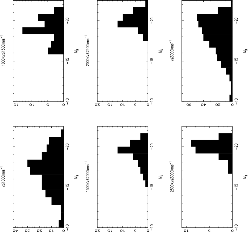
Figure 3: The distribution of total $R$-band absolute magnitudes for the observed galaxies. See Sect. 3 for details.

4 Data reduction

4.1 Flux measurements

The majority of the data reduction was performed using the Starlink package CCDPACK, with the rest making use of the Starlink KAPPA and FIGARO packages. The relevant commands were assembled into a set of executable scripts, streamlining the reduction process and ensuring that all data were treated in an objective and reproducible way. CCDPACK was used to perform bias subtraction, flat fielding by a median sky flat taken through the appropriate filter, image registration and co-addition (by median stacking to remove cosmic rays) for the multiple narrow-band images, and alignment of images taken in different filters, to remove systematic offsets which were found between different filters. All galaxy and standard star images were scaled to an effective integration time of 1 second to simplify photometric calculations.

One of the most critical stages of data reduction is the removal of the continuum contribution to the flux in the images taken through the narrow-band H$\alpha$ filters. The key parameter is the scaling factor applied to the image used for continuum subtraction (either an $R$-band or a H$\alpha$Cont image), which depends on the relative effective throughputs of the narrow-band and continuum filters to continuum light. These scaling factors were estimated in three ways. The first was to integrate numerically under the scanned, digitised filter profiles, which were already available for all the ING broad- and narrow-band filters; the ING kindly scanned the profile of the new H$\alpha$Cont filter in the same way. The ratio of these integrals for the narrow and continuum filters used for a specific galaxy observation then gives the scaling factor to be applied to the continuum image before it is subtracted from the narrow-band image. The second method was to use photometry of standard spectrophotometric stars through the pairs of filters in question, and using the ratio of counts per second detected to give the scaling factor. The third method was to calculate the ratio from foreground stars in the narrow-band and continuum images of each galaxy, thereby deriving a scaling factor which forces the cancellation of stellar images, at least in a statistical sense, in the continuum-subtracted images. This latter method has the advantage of accommodating any changes in the sky transparency between the two images, and can make use of several stars giving a statistical improvement in precision compared with using the standard stars. The drawback of this final method is that the colours of the stars used are not known, and may well be significantly bluer on average than the galaxy continuum, which would lead to a systematic error in the scaling factor. However, in practice it was found that the three methods gave very consistent values for the scaling factors, and the differences between them give good estimates of the likely errors in the continuum subtraction process. For non-photometric data, the final method (stars in the galaxy fields) was used to allow for sky transparency changes, but in photometric conditions standard ratios, calculated for every narrow/continuum filter pair from a combination of standard stars and field stars, were used, with the integrated filter profiles giving a strong consistency check. Good estimates of the scaling factors can be quickly obtained from the throughputs of the filters listed in the final column of Table 1, where the values are quoted as fractions of the $R$-band filter throughput.

Galactic extinction corrections were derived with the aid of NED, which uses data and methods from Schlegel et al. (schlegel (1998)) and Cardelli et al. (cardelli (1989)). These corrections were applied to the H$\alpha+$[Nii] fluxes prior to calculating star formation rates, but have not been applied to fluxes and magnitudes presented in this paper.

There is a known problem of light leaks with the JKT. This was only found to give significant problems when the moon was above the horizon, but did lead to some minor problems with gradients in the sky background. These were removed using a 2-dimensional polynomial fit to the background light, after removal of all stars and galaxies, using the KAPPA routine surfit. The fitted function was then subtracted from the original image, achieving both gradient removal and sky subtraction.

An extensive study was made into the dominant sources of errors on derived line fluxes and equivalent widths. The typical errors in total H$\alpha+$[Nii] fluxes due to background sky subtraction are 1%, with a worst-case error of 10%; filter throughput uncertainties are 9% (typical) or 15% (worst-case); continuum subtraction 10% (typical) or 35% (worst-case); and photometric errors from standard star observations 1.5% (typical) or 5% (worst-case). In calculating errors on H$\alpha+$[Nii] fluxes on a galaxy by galaxy basis, it was found that only the continuum subtraction and filter throughput errors contributed significantly to the totals, and given the importance of the first of these, the errors are strongly dependent on the EW of the H$\alpha+$[Nii] emission. For high EW ($>$2 nm) the total flux errors were calculated to be 10% or 15%, with the lower value being for the lower redshift galaxies. For low EW galaxies ($<$2 nm) the corresponding errors were calculated to be 25% and 35% respectively. The same percentage errors were allocated the the EW measurements, as in all cases the fractional errors on the continuum flux levels are much smaller than the fractional errors on line fluxes. The minimum detectable H$\alpha+$[Nii] EW is 0.2 nm, and the minimum line flux is 10^-17W m^-2.

Photometric calibration for the $R$-band images was quite straightforward, with the observations of Landolt standards being used to define zero-points and airmass corrections for each night in the usual way. Airmass corrections were generally very small, as most of the galaxy observations were made at airmass $<$1.5. Photometric calibration of the narrow-band continuum subtracted images is inevitably more involved, and the interested reader is referred to Shane (shane (2002)) for full details. In outline, the procedure was to tie the calibration of the H$\alpha$ fluxes to the Landolt standards observed on the same night, taking into account the transmission profiles of the filters used to both normalise the response to continuum sources through the $R$ filter, and to normalise the throughput of the narrow-band filter to the H$\alpha$ line. This latter is a function of the recession velocity of the galaxy, and it was assumed that all the line emission occurred at a wavelength corresponding to 6563 Å redshifted by the systemic recession velocity of the galaxy as listed in NED. This value will be slightly in error for the satellite [Nii] lines, and for specific Hii regions due to galaxy rotation, but such effects are small. This calculation thus accounts for overall transmission differences between filters used, and for the effect of the transmission profile on the specific line of interest. The latter has not been done in several previous studies, due to the lack of sufficiently accurate filter transmission data. The derived value for H$\alpha$ transmission was corrected, where appropriate, for the effective subtraction of a small part of the line flux along with the continuum, when the $R$-band filter was used to derive the continuum. The effect of this was minor, reducing the throughput to H$\alpha$ by about 3%. All line fluxes quoted in this paper have been corrected for this effect.

The net result of the calibration process is that the detected counts second^-1 in the $R$-band frames can be converted into either $R$-band magnitudes or flux densities in W m^-2 nm^-1, and in the H$\alpha$ continuum subtracted frames they can be directly converted to line fluxes in W m^-2. Both calibrations include all airmass, telescope, instrumental and filter transmission corrections.

The errors given on apparent $R$ magnitudes in this paper include contributions from the photometric zero point error for the given night, calculated from the scatter in standard star magnitudes, and from the error in determining the sky level on each image. This latter effect gives an error that varies as a function of galaxy magnitude and surface brightness. As a result we find that the total errors range from a of 0.04 mag for the brightest galaxies to 0.10 mag for low-surface-brightness dwarfs. Even for these latter galaxies, the errors due to photon shot noise are negligible and were not included in the error estimation.

Initial galaxy photometry was obtained within the Starlink GAIA package, using a set of between 30 and 60 concentric apertures ranging from 3$\aas@@fstack{\prime\prime}$3 up to between 100^′′ and 200^′′ in radius/semi-major axis, with the upper limit depending on the angular size of the galaxy. All apertures used, and hence all profiles calculated, are centred on the R-band galaxy centres. For irregular galaxies and face-on spiral galaxies, circular apertures were used, and for inclined spiral galaxies, elliptical apertures were used to obtain the data presented here. The ellipse parameters (ellipticity and major axis) were taken from the UGC, and checked by eye to ensure that they were a good fit to the present images. From this photometry, growth curves were constructed, both in $R$-band and H$\alpha+$[Nii] light. Dividing the H$\alpha+$[Nii] aperture fluxes by the corresponding $R$-band flux densities enables an estimate to be made of the H$\alpha+$[Nii] EW, assuming that the average continuum level within the $R$ filter is equal to the continuum level at 6563 Å.

Line fluxes and R-band magnitudes quoted in this paper are total values, where the apertures were set by requiring that the enclosed flux varied by less than 0.5% over 3 consecutive points in the H$\alpha+$[Nii] growth curves. Inspection of the apertures thus defined showed this to be a conservative criterion which encompassed all visible Hii regions; examples of these apertures are shown in figures later in this paper.

4.2 Comparison with literature measurements

Table 2: Repeat observations; asterisks indicate the adopted measurements for these galaxies.

$$\begin{array}[]{lcc|lcc}\hline\cr\vskip 3.0pt plus 1.0pt minus 1.0pt\cr${\bf Name}$&&&${\bf Name}$&&\\ $Obs. date $&$H$\alpha+$[N{\sc ii}] flux$&$H$\alpha+$[N{\sc ii}] EW$&$Obs. date $&$H$\alpha+$[N{\sc ii}] flux$&$H$\alpha+$[N{\sc ii}] EW$\\ &$(10$^{-16}$\leavevmode\nobreak\ W\leavevmode\nobreak\ m$^{-2}$)$&$(nm)$&&$(10$^{-16}$\leavevmode\nobreak\ W\leavevmode\nobreak\ m$^{-2}$)$&$(nm)$\\ \vskip 3.0pt plus 1.0pt minus 1.0pt\cr\hline\cr\vskip 3.0pt plus 1.0pt minus 1.0pt\cr${\bf UGC\leavevmode\nobreak\ 2023}$&&&${\bf UGC\leavevmode\nobreak\ 4115}$&&\\ 22/11/00*&3.440&3.7&19/11/00*&2.450&3.4\\ 18/12/00&2.610&2.4&20/11/00&2.299&3.4\\ \hline\cr${\bf UGC\leavevmode\nobreak\ 4173}$&&&${\bf UGC\leavevmode\nobreak\ 4469}$&&\\ 22/11/00*&2.041&5.8&17/02/01&8.948&2.7\\ 17/12/00&1.339&4.0&20/10/01*&9.771&4.5\\ \hline\cr${\bf UGC\leavevmode\nobreak\ 4484}$&&&${\bf UGC\leavevmode\nobreak\ 6251}$&&\\ 14/02/01&8.781&2.0&28/03/01*&1.795&4.7\\ 22/10/01*&6.057&1.7&11/05/01&1.391&4.6\\ \hline\cr${\bf UGC\leavevmode\nobreak\ 7232}$&&&${\bf UGC\leavevmode\nobreak\ 8188}$&&\\ 19/01/01*&4.685&2.0&09/05/00*&8.479&4.0\\ 03/04/01&7.004&3.2&28/03/01&5.657&2.0\\ \hline\cr${\bf UGC\leavevmode\nobreak\ 11331}$&&&${\bf UGC\leavevmode\nobreak\ 11332}$&&\\ 18/05/01&1.013&2.7&18/05/01&10.34&6.2\\ 22/10/01*&0.927&2.9&22/10/01*&10.57&5.0\\ \hline\cr${\bf UGC\leavevmode\nobreak\ 12294}$&&&${\bf NGC2604b}$&&\\ 04/08/01&25.57&4.2&14/02/01&0.490&1.4\\ 23/10/01*&31.63&4.4&20/10/01*&0.682&2.4\\ \vskip 3.0pt plus 1.0pt minus 1.0pt\cr\hline\cr\end{array}$$

In order to test our photometry, extensive internal and external comparison tests were performed. Table 2 shows the total measured H$\alpha+$[Nii] fluxes and line EWs for galaxies observed by us on more than one occasion, as a test of the internal reliability of the photometry in this study. These repeats give a conservative indication of the internal errors in the photometry for this study, as many of the measurements in the table were repeated due to doubts about the observing conditions for the first set of observations. UGC 2023 (18/12/00 observation) and UGC 7232 (03/07/01) both suffer from an unexplained ‘creased’ pattern in the narrow-band filter images. The observations of UGC 8188 (28/03/01), UGC 11331 (18/05/01) and UGC 11332 (18/05/01) for various reasons only resulted in two usable H$\alpha$ integrations, instead of the three needed to achieve a good signal-to-noise ratio and to remove cosmic-ray contamination. The mean variations shown by the 12 pairs of repeats are 29% in H$\alpha+$[Nii] flux, and 38% in EW. For the three galaxies which were observed on two photometric nights with no major problems (UGC 4115, UGC 6251 and UGC 12294), the agreements between the two sets of measurements are much better (a mean difference of 17% in the H$\alpha+$[Nii] flux, and of only 2% in the EW).

Figure 4: Comparison of literature values for total galaxy H$\alpha+$[Nii] fluxes with values from the present study.

Figure 5: Comparison of literature values for total galaxy H$\alpha+$[Nii] EWs with values from the present study.

Figure 4 illustrates a comparison of 105 literature measurements of H$\alpha+$[Nii] fluxes with the equivalent values from the present study for the same galaxies. The literature data are taken from the following papers: Kennicutt & Kent (ken83 (1983), KK83); Gallagher et al. (gal84 (1984), GHT84); Kennicutt et al. (ken87 (1987), KKHHR87); Kennicutt ken92 (1992), K92; Romanishin (rom90 (1990), R90); Young et al. (young (1996), YAKLR96); and Lehnert & Heckman (lehn96 (1996), LH96). All of these studies quote H$\alpha+$[Nii] fluxes which are total or near total values using either CCD photometry or large aperture spectrophotometry, with apertures in the following ranges: KK83, most fluxes in a 3^′ aperture, remainder 2^′, 5^′ or 7^′; GHT84) fluxes in 2^′ apertures; KKHHR87, total fluxes within an observed field of 2$\aas@@fstack{\prime}$3 square or 2$\aas@@fstack{\prime}$7 square; K92, 4 objects in 0$\aas@@fstack{\prime}$75 apertures, remainder in range 1–2^′; R90, apertures from 1$\aas@@fstack{\prime}$3 to 4$\aas@@fstack{\prime}$8, with most close to 2^′; YAKLR96), apertures not quoted, but measured from CCD images with a field of 6^′ by 6^′ or 7^′ by 4^′ ; and LH96, no apertures quoted but they state that these are total fluxes, measured from CCD images. Where specific apertures are quoted, these tend to be somewhat smaller than the software apertures used in the present study for deriving total fluxes, and the CCD-based studies use cameras with smaller fields than that of the JKT CCD. This will tend to offset points somewhat to the right of the one-to-one correspondence, indicated by the diagonal solid line. Data from the present study shown in Fig. 4 have been corrected for Galactic extinction, where this was done in the comparison study (GHT84, KK83, KKHHR87 and LH96), but not otherwise, and no corrections for extinction internal to the galaxy concerned have been applied. The mean offset in Fig. 4 is 0.11 dex (0.21 dex relative to KK83 and KKHHR87; 0.055 dex relative to R90 and YAKLR96), in the sense that this study finds higher fluxes than literature studies, possibly due to the larger effective apertures used. The plotted points have an RMS scatter of 0.16 dex about the best-fit regression line, or 0.20 dex about the line representing perfect agreement. Given the above uncertainties and differences in reduction procedures, the agreement found in Fig. 4 is generally good, and uncertainties in the internal extinction corrections to H$\alpha$ fluxes probably dominate over photometric errors as the main error in derived star formation rates.

Figure 5 shows a comparison of the H$\alpha+$[Nii] EWs for 88 galaxies from the present study with literature values for the same galaxies, again showing reasonable agreement overall, but with significant scatter, particularly for low EW galaxies. These objects are often early-type galaxies where uncertainties in H$\alpha+$[Nii] flux measurements are high due to low H$\alpha$ emission and the presence of H$\alpha$ absorption. The mean offset in Fig. 5 is 0.10 dex, in the sense that this study finds rather higher EWs than literature studies. The plotted points have an RMS scatter of 0.21 dex about the best-fit regression line, or 0.36 dex about the line representing perfect agreement.

4.3 Calculation of star formation rates

For the present paper, we calculate star formation rates from total H$\alpha+$[Nii] luminosities using the same relationship as Kennicutt et al. (ken94 (1994)):

$${\rm SFR}(M_{\odot}\leavevmode\nobreak\ {\rm yr}^{-1})=7.94\times 10^{-35}L_{{\rm H\alpha}}({\rm W})$$

This transformation is appropriate under the assumption of solar abundances and a Salpeter initial mass function (Salpeter sal55 (1955)) over a range of stellar masses from 0.1–100 M_⊙, and does not include the effect of dust attenuation on measured line fluxes. The H$\alpha$ luminosities in the present study were corrected for internal extinction assuming a constant value of 1.1 mag for each galaxy, independent of type and inclination. This value was found to be appropriate for local galaxies in studies by Kennicutt & Kent (ken83 (1983)) although Niklas et al. (nikl97 (1997)) found a rather smaller value of A${}_{\rm H\alpha}=$0.8 mag. Corrections for contamination by the [Nii] lines which lie within the passband of our filters were applied using the H$\alpha$/(H$\alpha+$[Nii]) ratios derived spectrophotometrically by Kennicutt & Kent (ken83 (1983)): 0.75$\pm$0.12 for spiral galaxies and 0.93$\pm$0.05 for irregular galaxies. However, it should be noted that Tresse et al. (tres99 (1999)), in a very large spectroscopic study of local galaxies, find that this ratio varies systematically as a function of EW(H$\alpha+$[Nii]), in the sense that [Nii] is less significant in high-EW galaxies. These corrections can also be affected by the possible presence of high-excitation emission-line regions around AGN. The [Nii] and extinction corrections are applied only when calculating star formation rates in the present paper; hence any H$\alpha$ EW values and line fluxes presented here are in fact for H$\alpha+$[Nii], uncorrected for internal and Galactic extinction. All of these corrections will be examined in more detail in a later paper, but initial analysis of our data shows a good general agreement with the values obtained by Kennicutt and coworkers.

The errors on the star formation rates were derived from line flux errors discussed above, added in quadrature with errors resulting from distance uncertainties, and in most cases the latter was the dominant contribution. The distance error was taken as $\pm$25% for galaxies closer than 8 Mpc (corresponding to a 56% error in star formation rate), and as $\pm$2 Mpc for galaxies outside this distance.

5 Results

The main results in this paper are listed in Table 3, which contains the photometric data and derived star formation rates for the full sample of 334 galaxies. Column 1 contains the number of each galaxy in the Uppsala Galaxy Catalogue; col. 2 the Hubble type, taken from NED; col. 3 the heliocentric recession velocity from NED; col. 4 the distance in Mpc of the galaxy, assuming a Hubble constant of 75 km s^-1Mpc^-1 and after corrections from a Virgo infall model; col. 5 the galaxy major axis in minutes of arc, from NED; col. 6 the major-to-minor axis ratio, from NED; col. 7 the total $R$ magnitude derived from this study, with errors in brackets; col. 8 the total H$\alpha+$[Nii] flux, after all corrections described in the previous section except those for [Nii] contamination, Galactic extinction and internal extinction, in units of 10^-16W m^-2, and with errors given in brackets; col. 9 the EW in nm of the H$\alpha+$[Nii] lines, with errors in brackets; col. 10 contains the total star formation rate, based on the total measured H$\alpha+$[Nii] line flux corrected for [Nii] contamination, Galactic extinction and internal extinction, with the conversion factor as described in Sect. 4.3, and errors in brackets; and col. 11 contains H$\alpha+$[Nii] surface brightnesses within Petrosian radii, calculated as described in section 6.2, and with errors in brackets. The galaxies are listed in Right Ascension order, within each of the five recession velocity shells, starting with the lowest velocity shell (up to 1000 km s^-1). Serendipitously discovered galaxies are listed at the end of the table. Data for the different recession velocity shells are separated by a horizontal line in the table.

Table 3: *

Table 3. Photometric, distance and star formation data for 334 galaxies.
UGC	Class	$v_{\rm{rec}}$	Dist.	Dia	$a/b$	$m_{R}$	F(H$\alpha+$[Nii])	EW	SFR	SB$\times$10-20
		kms-1	Mpc	′		mag	10-16W m-2	nm	M⊙ yr-1	Wm-2/′′2
17	Sm	878	9.9	2.5	1.5	14.49(0.06)	2.1(0.21)	6.0(0.6)	0.0448(0.0204)	2.4(0.34)
75	IBm	865	9.7	2.8	1.3	12.33(0.04)	4.2(1.05)	1.6(0.4)	0.1167(0.0606)	5.2(1.40)
655	Sm	836	10.6	2.5	1.0	14.05(0.06)	0.9(0.22)	1.6(0.4)	0.0224(0.0108)	1.1(0.29)
891	SABm	643	7.2	2.3	2.3	14.05(0.06)	0.5(0.13)	1.0(0.3)	0.0059(0.0036)	0.6(0.17)
1176	Im	633	7.3	4.6	1.3	14.29(0.06)	1.8(0.18)	4.3(0.4)	0.0275(0.0156)	1.3(0.19)
1195	Im	774	8.8	3.4	3.1	13.35(0.05)	1.7(0.43)	1.8(0.4)	0.0386(0.0218)	1.8(0.47)
1200	IBm	808	9.2	2.0	1.4	13.19(0.05)	3.4(0.34)	3.0(0.3)	0.0795(0.0391)	7.4(1.05)
1865	Sm:	580	7.5	2.8	1.3	14.42(0.06)	1.1(0.11)	3.1(0.3)	0.0149(0.0085)	1.1(0.15)
1983	SAb:	609	8.0	2.4	1.8	11.49(0.04)	17.1(1.71)	3.1(0.3)	0.2471(0.1412)	19.5(2.76)
2002	Sdm:	597	7.8	2.3	1.6	12.00(0.04)	10.3(1.03)	3.0(0.3)	0.1467(0.0834)	6.8(0.96)
2017	Im	985	12.1	2.3	1.4	15.27(0.10)	0.2(0.10)	1.4(0.4)	0.0111(0.0060)	0.3(0.15)
2014	Im:	565	7.5	2.0	3.3	14.69(0.06)	0.9(0.10)	3.1(0.3)	0.0138(0.0078)	1.4(0.19)
2023	Im:	603	7.8	1.7	1.0	13.42(0.05)	3.5(0.35)	3.8(0.4)	0.0662(0.0377)	2.3(0.33)
2141	S0/a	987	12.2	2.5	2.3	12.02(0.04)	15.6(1.56)	4.6(0.5)	0.6539(0.2410)	10.9(1.54)
2193	SAc	518	6.9	3.0	1.1	11.08(0.04)	30.6(3.06)	3.8(0.4)	0.3330(0.1894)	21.7(3.06)
2455	IBm	375	4.9	3.3	1.3	11.91(0.04)	27.6(2.76)	7.4(0.7)	0.2800(0.1593)	36.8(5.20)
2684	Im	350	4.6	1.8	2.0	16.19(0.10)	0.2(0.10)	2.9(0.3)	0.0015(0.0010)	0.4(0.20)
2947	SBm	863	10.8	3.6	4.0	11.99(0.04)	12.9(1.29)	3.7(0.4)	0.4413(0.1839)	1.3(0.18)
3174	IABm:	670	9.2	1.7	1.5	15.36(0.10)	0.8(0.10)	5.3(0.5)	0.0214(0.0106)	1.3(0.19)
3371	Im:	816	13.3	4.6	1.3	14.73(0.06)	0.7(0.10)	2.4(0.2)	0.0418(0.0141)	0.6(0.10)
3429	SBab	893	14.5	6.0	1.8	10.06(0.04)	51.2(5.12)	2.5(0.2)	2.6773(0.8337)	11.3(1.60)
3711	IBm	436	7.6	2.2	1.3	12.29(0.04)	13.4(1.34)	5.1(0.5)	0.2339(0.1330)	26.1(3.69)
3734	SAc:	974	15.9	1.7	1.0	11.60(0.04)	3.4(0.85)	0.7(0.2)	0.2144(0.0785)	2.9(0.77)
3817	Im:	438	8.3	1.8	2.0	15.16(0.10)	0.8(0.10)	4.3(0.4)	0.0175(0.0096)	1.3(0.19)
3847	IRR	70	2.9	1.7	1.5	14.75(0.06)	9.2(0.92)	33.9(3.4)	0.0207(0.0118)	19.7(2.78)
3851	IBm	100	2.9	8.1	2.5	11.76(0.04)	101.7(10.2)	23.6(2.4)	0.2277(0.1295)	24.8(3.51)
3876	SAd	860	14.5	2.2	1.7	12.97(0.04)	3.5(0.35)	2.5(0.3)	0.1630(0.0508)	2.6(0.37)
3966	Im	361	6.2	1.7	1.0	14.51(0.06)	0.8(0.10)	2.4(0.2)	0.0087(0.0050)	0.9(0.12)
4115	IAm	338	5.8	1.8	1.8	13.70(0.05)	2.5(0.25)	3.5(0.3)	0.0221(0.0125)	2.3(0.32)
4165	SBd	514	9.0	2.9	1.1	11.51(0.04)	20.0(2.00)	3.7(0.4)	0.3518(0.1773)	9.9(1.40)
4173	Im:	860	14.3	1.9	3.2	14.48(0.06)	2.1(0.21)	6.0(0.6)	0.1122(0.0354)	1.5(0.21)
4274	SBm	447	7.7	1.7	1.1	11.40(0.04)	24.7(2.47)	4.1(0.4)	0.3280(0.1866)	43.5(6.15)
4325	SAm	524	9.2	3.5	1.5	12.59(0.04)	6.6(0.66)	3.3(0.3)	0.1222(0.0601)	3.9(0.55)
4426	Im:	397	6.7	2.0	2.0	14.72(0.06)	0.8(0.10)	3.0(0.3)	0.0100(0.0057)	0.9(0.12)
4499	SABd	691	12.2	2.6	1.4	13.06(0.05)	6.4(0.64)	4.9(0.5)	0.2047(0.0754)	5.0(0.70)
4514	SBcd	691	12.2	2.1	2.3	13.18(0.05)	3.4(0.34)	2.9(0.3)	0.1072(0.0395)	1.6(0.23)
4645	SAB0/a	692	12.3	3.6	1.1	10.04(0.04)	18.1(4.53)	0.9(0.2)	0.5675(0.2449)	11.3(3.05)
4879	IAm	600	10.5	1.7	1.3	13.18(0.05)	0.2(0.10)	0.2(0.2)	0.0050(0.0024)	0.1(0.05)
5139	IABm	143	2.3	3.6	1.2	13.71(0.05)	4.0(0.40)	5.5(0.6)	0.0058(0.0033)	0.7(0.10)
5221	SAc	3	2.1	5.9	2.2	10.21(0.04)	62.4(6.24)	3.5(0.3)	0.0641(0.0365)	12.8(1.82)
5272	Im	520	7.7	2.1	2.6	13.78(0.05)	4.1(0.41)	6.2(0.6)	0.0629(0.0358)	4.5(0.64)
5340	Im	503	7.2	2.7	2.7	14.14(0.06)	2.6(0.26)	5.3(0.5)	0.0339(0.0193)	2.6(0.36)
5336	Im	46	3.4	2.5	1.3	13.88(0.05)	1.1(0.27)	1.8(0.4)	0.0035(0.0022)	0.4(0.10)
5364	IBm	20	1.0	5.1	1.6	13.58(0.05)	3.3(0.33)	4.1(0.4)	0.0008(0.0005)	1.7(0.24)
5373	Im	301	3.9	5.1	1.5	12.58(0.04)	7.3(0.73)	3.6(0.4)	0.0291(0.0165)	4.0(0.57)
5398	I0	14	2.1	5.4	1.2	10.35(0.04)	66.2(6.62)	4.2(0.4)	0.0838(0.0477)	40.6(5.74)
5414	IABm	603	9.5	3.2	1.5	13.07(0.05)	6.4(0.64)	4.9(0.5)	0.1443(0.0687)	4.0(0.56)
5637	IBm	753	10.8	5.0	1.5	11.07(0.04)	49.9(4.99)	6.2(0.6)	1.5315(0.6384)	19.2(2.71)
5672	Sab	531	6.8	1.8	3.6	13.72(0.05)	1.5(0.15)	2.2(0.2)	0.0147(0.0083)	1.3(0.18)
5692	Sm:	180	2.9	3.2	1.8	13.67(0.05)	1.8(0.18)	2.5(0.2)	0.0034(0.0019)	1.9(0.27)
5721	SABd	537	6.9	2.1	2.1	12.16(0.04)	12.2(1.22)	4.1(0.4)	0.1213(0.0690)	7.5(1.06)
5719	SBdm:	941	17.1	2.9	2.4	13.14(0.05)	7.1(0.71)	5.9(0.6)	0.4179(0.1116)	2.5(0.35)
5740	SABm	649	10.9	1.7	1.4	13.67(0.05)	2.3(0.23)	3.1(0.3)	0.0558(0.0231)	1.8(0.25)
5761	SABdm	641	8.1	2.2	1.3	12.20(0.04)	3.7(0.92)	1.3(0.3)	0.0506(0.0308)	2.8(0.75)
5764	IBm:	586	7.8	2.0	1.8	14.57(0.06)	1.5(0.15)	4.6(0.5)	0.0234(0.0133)	2.6(0.37)
5786	SABbc	993	18.2	3.1	1.3	10.40(0.04)	163.4(16.3)	10.9(1.1)	11.231(2.8359)	477.6(7.54)
5829	Im	629	8.6	4.7	1.1	13.13(0.05)	15.0(1.50)	12.3(1.2)	0.2859(0.1512)	3.7(0.53)
5848	Sm:	822	14.9	2.1	2.1	14.09(0.06)	1.4(0.14)	2.8(0.3)	0.0624(0.0189)	1.3(0.18)
5889	SABm	572	6.9	2.2	1.0	13.63(0.05)	1.2(0.30)	1.5(0.4)	0.0120(0.0074)	0.9(0.24)
5918	Im:	340	5.4	2.4	1.0	14.52(0.06)	0.7(0.10)	2.0(0.2)	0.0050(0.0029)	0.5(0.07)
6123	SBb	979	20.9	3.4	1.2	10.80(0.04)	40.5(4.05)	3.9(0.4)	3.6838(0.8255)	18.6(2.63)
6161	SBdm	756	12.3	2.6	2.2	13.52(0.05)	2.9(0.29)	3.4(0.3)	0.0881(0.0322)	1.6(0.22)
6251	SABm:	927	17.1	1.8	1.1	14.39(0.06)	1.8(0.18)	4.6(0.5)	0.1050(0.0280)	1.8(0.26)
6272	SA0/a:	628	7.1	5.2	2.7	10.70(0.04)	29.4(2.94)	2.6(0.3)	0.3052(0.1736)	11.0(1.55)
6399	Sm:	805	14.4	2.8	3.5	13.27(0.05)	2.6(0.26)	2.5(0.2)	0.1122(0.0352)	0.9(0.13)
6439	SAb	770	12.2	5.9	1.9	10.08(0.04)	35.2(8.80)	1.8(0.4)	1.0789(0.4682)	7.0(1.90)
6446	SAd	645	10.5	3.5	1.5	13.88(0.05)	4.9(0.49)	8.0(0.8)	0.1095(0.0470)	6.7(0.95)
6565	Irr	229	3.1	2.5	1.3	11.68(0.04)	16.1(1.61)	3.5(0.3)	0.0388(0.0221)	17.3(2.45)
6572	Im	229	2.9	2.0	1.8	13.77(0.05)	4.4(0.44)	6.6(0.7)	0.0097(0.0055)	8.0(1.14)
6595	SBb:	732	11.8	3.1	3.1	11.69(0.04)	13.3(1.33)	2.9(0.3)	0.3855(0.1469)	5.3(0.75)
6618	SABcd:	739	11.7	1.7	1.5	12.55(0.04)	11.1(1.11)	5.3(0.5)	0.3120(0.1199)	9.8(1.39)
6628	SAm	850	15.2	2.9	1.0	12.38(0.04)	5.8(0.58)	2.4(0.2)	0.2811(0.0837)	2.1(0.29)
6644	SAc	993	16.9	4.3	1.4	10.39(0.04)	67.3(6.73)	4.4(0.4)	4.2056(1.1351)	20.6(2.92)
6670	IBm	922	17.6	3.0	3.3	12.63(0.04)	12.0(1.20)	6.2(0.6)	0.9595(0.2496)	13.6(1.92)
6778	SABc:	977	18.5	4.5	1.6	10.35(0.04)	79.4(7.94)	5.0(0.5)	5.6248(1.3999)	30.2(4.27)
6781	SB0/a:	905	18.5	1.4	1.4	13.05(0.05)	2.0(0.51)	1.5(0.4)	0.1432(0.0484)	4.4(1.17)
6782	Im	525	5.7	2.0	1.0	15.71(0.10)	0.6(0.10)	4.9(0.5)	0.0047(0.0027)	1.1(0.15)
6797	SBd	961	18.2	1.9	1.1	12.33(0.04)	6.8(0.68)	2.7(0.3)	0.4688(0.1184)	7.7(1.09)
6813	SAd:	954	17.7	2.6	1.0	12.60(0.04)	4.9(0.49)	2.5(0.2)	0.3105(0.0804)	5.5(0.78)
6815	SAcd:	968	18.1	5.1	3.9	11.58(0.04)	7.6(1.89)	1.5(0.4)	0.5124(0.1752)	0.4(0.12)
6818	SBb	819	14.0	2.0	2.0	13.58(0.05)	2.2(0.22)	2.8(0.3)	0.0913(0.0294)	0.5(0.07)
6817	Im	243	2.9	4.1	2.7	13.90(0.05)	3.6(0.36)	6.0(0.6)	0.0078(0.0044)	2.0(0.28)
6824	S0/a	906	16.9	1.7	2.1	12.28(0.04)	1.2(0.30)	0.4(0.2)	0.0710(0.0251)	1.5(0.40)
6833	SABc	919	17.6	3.2	1.3	12.67(0.04)	25.0(2.50)	13.5(1.4)	1.6029(0.4170)	13.7(1.94)
6869	SAbc:	807	13.9	2.9	1.7	10.70(0.04)	60.2(6.02)	5.3(0.5)	2.4053(0.7800)	54.3(7.68)
6900	Sd	590	6.8	2.1	1.6	13.93(0.05)	0.6(0.15)	1.0(0.3)	0.0056(0.0034)	0.4(0.11)
6904	SAbc	842	15.4	3.9	3.5	11.94(0.04)	9.8(0.98)	2.7(0.3)	0.4702(0.1383)	1.1(0.16)
6917	SBm	910	17.0	3.5	1.8	13.20(0.05)	1.9(0.47)	1.6(0.4)	0.1143(0.0404)	1.4(0.37)
6930	SABd	778	13.2	4.4	1.6	12.46(0.04)	8.6(0.86)	3.8(0.4)	0.3173(0.1082)	5.3(0.75)
6956	SBm	917	17.1	2.2	1.0	14.43(0.06)	1.1(0.11)	2.9(0.3)	0.0642(0.0171)	0.8(0.12)
6955	IBm:	905	16.5	5.0	1.9	13.32(0.05)	2.0(0.50)	2.0(0.5)	0.1372(0.0492)	1.1(0.30)
6962	SABcd	784	11.8	2.3	1.2	11.89(0.04)	13.8(1.38)	3.6(0.4)	0.3969(0.1512)	9.1(1.29)
6973	Sab:	701	9.7	2.6	2.2	11.28(0.04)	17.2(1.72)	2.6(0.3)	0.3340(0.1555)	20.4(2.88)
7002	SBb:	932	17.5	2.5	1.3	12.09(0.04)	6.2(1.56)	2.0(0.5)	0.4029(0.1401)	3.5(0.94)
7007	Sm:	774	9.4	1.7	1.1	14.14(0.06)	0.3(0.10)	0.7(0.2)	0.0063(0.0034)	0.3(0.10)
7030	SABbc	725	10.6	5.2	1.3	10.05(0.04)	66.3(6.63)	3.2(0.3)	1.5093(0.6413)	14.2(2.01)
7047	IAm	210	2.8	3.3	1.9	12.59(0.04)	9.0(0.90)	4.5(0.5)	0.0182(0.0103)	5.7(0.80)
7045	SAc	769	9.1	4.1	2.4	10.70(0.04)	22.3(5.57)	2.0(0.5)	0.3850(0.2111)	2.2(0.61)
7054	SBa:	913	17.6	4.4	2.6	11.04(0.04)	10.8(2.70)	1.3(0.3)	0.6917(0.2398)	3.1(0.83)
7075	SABc:	752	12.6	2.8	3.5	11.86(0.04)	21.7(2.17)	5.6(0.6)	0.7076(0.2526)	2.4(0.34)
7081	SABbc	760	12.9	5.8	2.6	10.08(0.04)	89.1(8.91)	4.4(0.4)	3.0566(1.0660)	14.7(2.09)
7096	SABb	837	15.2	3.0	1.8	10.47(0.04)	36.5(3.65)	2.6(0.3)	1.7388(0.5178)	22.5(3.18)
7134	SABc	609	6.8	4.0	1.1	11.27(0.04)	15.0(1.50)	2.2(0.2)	0.1423(0.0809)	5.9(0.83)
7151	SABcd	265	3.3	6.0	4.6	11.32(0.04)	23.2(2.32)	3.6(0.4)	0.0514(0.0292)	9.8(1.39)
7199	IAm	165	1.9	1.8	1.1	12.87(0.04)	1.3(0.32)	0.8(0.2)	0.0012(0.0007)	1.6(0.42)
7215	SBdm	378	3.9	5.1	2.8	11.09(0.04)	37.0(3.70)	4.6(0.5)	0.1181(0.0672)	2.5(0.35)
7216	SBcd:	-183	17.4	1.9	2.4	13.69(0.05)	2.5(0.25)	3.5(0.3)	0.1657(0.0436)	1.6(0.23)
7232	Im	228	2.6	1.7	1.1	12.42(0.04)	4.8(0.48)	2.0(0.2)	0.0085(0.0048)	5.2(0.74)
7261	SBdm	861	9.0	3.6	1.2	12.43(0.04)	16.4(1.64)	7.1(0.7)	0.2835(0.1428)	5.1(0.72)
7267	Sdm:	472	6.6	2.1	2.6	13.73(0.05)	1.2(0.31)	1.8(0.4)	0.0111(0.0068)	1.1(0.29)
7271	SBd:	546	7.0	2.0	3.3	13.89(0.05)	1.1(0.28)	1.9(0.5)	0.0112(0.0069)	0.4(0.12)
7315	SABbc	867	17.6	2.1	1.6	11.18(0.04)	13.2(3.30)	1.8(0.4)	0.8649(0.2998)	10.8(2.91)
7323	SABdm	517	6.8	5.0	1.3	11.29(0.04)	11.6(2.90)	1.8(0.4)	0.1088(0.0667)	1.9(0.51)
7326	Im:	-164	17.4	1.9	3.2	15.29(0.10)	1.2(0.12)	7.3(0.7)	0.0963(0.0253)	2.3(0.32)
7328	SB0/a:	890	10.4	2.9	1.3	10.82(0.04)	9.0(2.24)	0.9(0.2)	0.2001(0.0981)	9.0(2.42)
7405	SB0/a	893	17.6	5.6	2.2	10.25(0.04)	11.6(2.89)	0.7(0.2)	0.7765(0.2692)	2.2(0.59)
7414	SABdm:	232	2.4	1.7	1.1	12.03(0.04)	25.5(2.55)	7.6(0.8)	0.0312(0.0178)	32.3(4.56)
7523	SBb	922	17.5	3.6	1.1	10.52(0.04)	13.6(3.40)	1.0(0.3)	0.8852(0.3078)	5.3(1.42)
7539	SAc	716	8.2	3.6	1.8	9.61(0.04)	72.1(7.21)	2.3(0.2)	0.9977(0.5551)	30.0(4.24)
7559	IBm	218	2.5	3.2	1.6	13.62(0.05)	4.0(0.40)	5.1(0.5)	0.0063(0.0036)	2.1(0.29)
7561	SBa:	439	4.6	3.6	2.0	11.80(0.04)	9.4(0.94)	2.3(0.2)	0.0410(0.0233)	7.3(1.04)
7622	SB0/a	508	18.8	3.8	2.9	11.14(0.04)	6.1(1.53)	0.8(0.2)	0.4439(0.1490)	1.8(0.47)
7690	Im:	537	6.8	1.7	1.1	12.45(0.04)	5.6(0.56)	2.5(0.2)	0.0681(0.0387)	5.8(0.82)
7753	SBb	486	18.1	5.4	1.3	9.95(0.04)	18.7(4.68)	0.8(0.2)	1.3205(0.4514)	2.9(0.78)
7826	SABb	631	18.0	1.7	1.5	11.80(0.04)	7.7(1.92)	1.9(0.5)	0.5352(0.1835)	8.7(2.35)
7866	IABm	359	4.2	3.4	1.1	13.80(0.05)	3.3(0.33)	5.0(0.5)	0.0148(0.0084)	3.4(0.48)
7874	SABdm:	291	3.0	2.1	2.3	13.10(0.05)	4.9(0.49)	3.9(0.4)	0.0092(0.0053)	2.4(0.34)
7901	SAc	805	17.8	4.0	1.5	10.33(0.04)	37.1(3.71)	2.3(0.2)	2.4632(0.6344)	21.4(3.02)
7971	Sm:	467	6.5	2.2	1.0	13.45(0.05)	3.0(0.30)	3.3(0.3)	0.0255(0.0145)	1.8(0.25)
7985	SABd	652	6.8	2.7	1.6	11.29(0.04)	41.0(4.10)	6.2(0.6)	0.3985(0.2267)	24.4(3.45)
8024	IBm	376	4.1	3.0	1.4	13.46(0.05)	4.2(0.42)	4.7(0.5)	0.0177(0.0101)	2.4(0.34)
8034	Im	915	17.6	1.7	1.9	13.61(0.05)	6.3(0.63)	8.0(0.8)	0.5142(0.1338)	10.1(1.42)
8054	SAcd:	778	20.7	2.8	2.5	11.46(0.04)	30.5(3.05)	5.4(0.5)	2.8064(0.6340)	19.3(2.73)
8098	SBm:	847	11.0	4.0	2.7	12.35(0.04)	45.6(4.57)	18.2(1.8)	1.1130(0.4553)	6.2(0.88)
8116	SBc	969	17.1	2.2	1.0	10.96(0.04)	38.0(3.80)	4.2(0.4)	2.3140(0.6179)	33.2(4.70)
8188	SAm	321	3.7	6.0	1.1	12.53(0.04)	8.7(0.87)	4.1(0.4)	0.0242(0.0138)	1.2(0.17)
8201	Im	37	2.8	3.5	1.8	13.06(0.05)	1.3(0.32)	1.0(0.2)	0.0025(0.0015)	0.6(0.16)
8256	SABbc	946	18.9	5.8	2.1	9.46(0.04)	44.1(11.0)	1.2(0.3)	3.1988(1.0713)	8.4(2.25)
8303	IABm	944	18.9	2.2	1.2	13.11(0.05)	7.8(0.78)	6.3(0.6)	0.7073(0.1728)	6.2(0.87)
8313	SBc	625	8.3	1.7	4.3	13.52(0.05)	3.3(0.33)	3.9(0.4)	0.0463(0.0254)	2.2(0.30)
8320	IBm	195	2.4	3.6	2.6	12.82(0.04)	6.0(0.60)	3.7(0.4)	0.0087(0.0049)	3.8(0.53)
8331	IAm	260	3.3	2.7	3.0	13.79(0.05)	1.7(0.17)	2.6(0.3)	0.0046(0.0026)	1.7(0.24)
8396	SBd	946	18.6	1.7	3.4	13.06(0.05)	10.7(1.07)	8.3(0.8)	0.7517(0.1862)	9.8(1.39)
8403	SBcd	965	19.1	4.0	1.4	11.49(0.04)	29.0(2.90)	5.2(0.5)	2.1315(0.5159)	7.7(1.09)
8490	SAm	201	2.8	5.0	1.7	11.44(0.04)	31.3(3.13)	5.4(0.5)	0.0496(0.0282)	7.1(1.01)
8508	IAm	62	2.7	1.7	1.7	13.41(0.05)	3.6(0.36)	3.8(0.4)	0.0065(0.0037)	4.7(0.66)
8565	SABdm	232	3.1	1.7	1.2	13.24(0.05)	4.0(0.40)	3.6(0.4)	0.0077(0.0044)	3.3(0.47)
8760	Im	193	2.3	2.2	3.1	13.80(0.05)	0.7(0.19)	1.1(0.3)	0.0010(0.0006)	0.5(0.14)
8837	IBm	144	3.9	4.3	3.3	12.07(0.04)	4.5(1.12)	1.4(0.3)	0.0172(0.0105)	1.4(0.36)
8839	Im	957	20.5	4.0	1.5	14.01(0.06)	0.2(0.10)	0.5(0.2)	0.0271(0.0140)	2.6(1.30)
9013	SAcd	273	3.8	4.8	1.1	10.80(0.04)	22.8(2.28)	2.2(0.2)	0.0664(0.0378)	5.6(0.79)
9018	SAm	304	4.3	1.7	1.3	13.64(0.05)	7.0(0.70)	9.2(0.9)	0.0261(0.0148)	8.2(1.15)
9128	Im	154	2.2	1.7	1.3	13.86(0.05)	0.4(0.10)	0.6(0.2)	0.0005(0.0003)	0.3(0.10)
9179	SABd	305	4.5	5.8	1.6	11.21(0.04)	28.5(2.86)	4.0(0.4)	0.1179(0.0671)	5.3(0.75)
9211	Im:	686	11.2	1.7	1.2	15.00(0.10)	3.6(0.91)	—	0.1129(0.0522)	—
9219	Im:	663	10.2	2.6	2.0	13.17(0.05)	4.7(0.47)	4.0(0.4)	0.1220(0.0539)	8.3(1.18)
9240	IAm	150	3.7	1.8	1.0	12.98(0.04)	3.7(0.37)	2.7(0.3)	0.0128(0.0073)	3.5(0.49)
9405	Im	222	3.2	1.7	2.8	14.24(0.06)	0.8(0.20)	1.8(0.4)	0.0020(0.0012)	0.9(0.23)
9649	SBb	447	7.7	3.7	1.7	11.77(0.04)	8.7(0.87)	2.0(0.2)	0.1083(0.0616)	3.1(0.44)
9753	SAbc:	772	13.8	4.2	3.2	11.42(0.04)	16.7(1.67)	2.8(0.3)	0.6413(0.2094)	8.9(1.26)
9769	SABdm:	841	15.1	2.7	1.4	13.34(0.05)	1.9(0.46)	1.9(0.5)	0.0861(0.0325)	1.0(0.27)
9866	SAbc	435	7.4	2.2	2.2	11.78(0.04)	9.6(0.96)	2.3(0.2)	0.1089(0.0620)	7.4(1.05)
9906	Sc	656	11.6	3.3	1.3	12.18(0.04)	13.0(1.30)	4.4(0.4)	0.3515(0.1363)	49.7(7.03)
10075	SAcd	835	14.7	5.4	2.6	10.96(0.04)	27.4(2.74)	3.1(0.3)	1.1993(0.3686)	4.6(0.66)
10310	SBm	716	12.7	2.8	1.3	13.08(0.05)	8.0(0.80)	6.3(0.6)	0.2610(0.0924)	4.0(0.57)
10445	SBc	963	16.9	2.8	1.6	12.89(0.04)	7.8(0.78)	5.1(0.5)	0.4732(0.1277)	10.7(1.52)
10521	SAc	852	15.0	3.0	2.3	11.24(0.04)	36.7(3.67)	5.3(0.5)	1.6847(0.5079)	17.3(2.45)
10606	SBcd:	919	15.9	3.6	2.4	14.21(0.06)	3.9(0.39)	8.7(0.9)	0.2017(0.0576)	1.0(0.14)
10736	SABdm	490	8.6	3.1	3.4	13.92(0.05)	1.0(0.24)	1.6(0.4)	0.0153(0.0088)	0.6(0.16)
10806	SBdm	932	15.7	2.1	2.3	12.76(0.04)	6.7(0.67)	3.9(0.4)	0.3469(0.1002)	2.2(0.31)
11300	SBcd	490	8.4	3.8	2.9	12.29(0.04)	7.6(0.76)	2.9(0.3)	0.1241(0.0673)	1.1(0.16)
12048	IBm	986	12.2	2.1	1.2	12.15(0.04)	16.6(1.66)	5.6(0.6)	0.7043(0.2596)	16.2(2.30)
12082	Sm	802	10.1	2.6	1.2	13.47(0.05)	2.7(0.27)	3.1(0.3)	0.0694(0.0310)	1.5(0.21)
12101	SAd	786	9.9	2.2	2.0	12.63(0.04)	7.2(0.72)	3.7(0.4)	0.1671(0.0762)	7.0(0.99)
12613	Im	-183	1.0	5.0	1.9	14.89(0.06)	0.1(0.10)	0.4(0.2)	.00002(.00002)	.01(0.01)
12732	Sm:	749	8.9	3.0	1.1	13.70(0.05)	6.3(0.63)	8.8(0.9)	0.1220(0.0622)	5.7(0.80)
12754	SBcd	751	8.9	4.4	1.5	11.45(0.04)	26.5(2.64)	4.6(0.5)	0.4936(0.2516)	6.9(0.98)
12893	SAdm	1108	12.5	1.7	1.0	13.33(0.05)	0.4(0.10)	0.4(0.2)	0.0121(0.0051)	0.4(0.11)
763	SABm	1162	12.7	5.1	1.4	11.38(0.04)	19.4(1.94)	3.2(0.3)	0.6567(0.2326)	9.9(1.40)
2053	Im	1029	12.7	2.0	2.0	14.40(0.06)	0.4(0.10)	1.0(0.3)	0.0205(0.0087)	0.4(0.10)
2210	SBc	1211	13.9	4.9	1.1	11.57(0.04)	26.3(2.63)	5.1(0.5)	1.0953(0.3552)	6.1(0.86)
2275	Sm:	1025	11.9	7.5	1.4	17.52(0.10)	0.2(0.10)	11.1(1.1)	0.0081(0.0031)	0.2(0.10)
2302	SBm:	1104	12.8	4.8	1.3	14.37(0.06)	8.0(0.80)	20.5(2.1)	0.3119(0.1096)	7.1(1.00)
2855	SABc	1202	17.5	4.4	2.2	11.11(0.04)	26.5(2.65)	3.4(0.3)	9.7830(2.5583)	9.4(1.33)
3384	Sm:	1089	17.0	1.7	1.0	14.68(0.06)	1.3(0.13)	4.6(0.5)	0.1229(0.0330)	1.8(0.25)
3403	SBcd	1264	19.2	2.7	3.4	13.02(0.05)	3.3(0.33)	2.5(0.2)	0.4179(0.1007)	1.3(0.18)
3439	SABc:	1494	22.3	3.3	2.7	12.81(0.04)	2.8(0.71)	1.7(0.4)	0.3503(0.1094)	1.1(0.31)
3574	SAcd	1441	21.8	4.2	1.2	12.21(0.04)	6.1(0.61)	2.2(0.2)	0.6487(0.1404)	3.4(0.47)
3580	SAa:	1201	18.8	3.6	2.3	12.44(0.04)	6.7(0.67)	2.9(0.3)	0.5300(0.1301)	6.5(0.92)
4097	SAa	1442	22.5	1.9	1.3	11.33(0.04)	4.6(1.15)	0.7(0.2)	0.5461(0.1701)	8.6(2.31)
4121	Sm:	1092	18.0	2.0	2.5	15.14(0.10)	0.4(0.10)	1.9(0.5)	0.0243(0.0083)	0.3(0.08)
4637	SAB0/a	1404	21.8	4.9	1.2	11.20(0.04)	2.0(0.49)	0.3(0.2)	0.1961(0.0618)	—
4781	Scd:	1443	24.3	1.7	2.8	14.40(0.06)	1.4(0.14)	3.7(0.4)	0.1794(0.0356)	1.2(0.17)
4779	SAc:	1289	21.3	3.2	1.9	11.15(0.04)	15.9(1.59)	2.1(0.2)	1.5585(0.3438)	3.8(0.54)
5349	Sdm:	1381	24.4	2.5	2.8	13.30(0.05)	3.3(0.33)	3.2(0.3)	0.4020(0.0795)	1.5(0.21)
5393	SBdm:	1448	25.5	1.9	1.7	13.54(0.05)	2.7(0.27)	3.2(0.3)	0.3498(0.0669)	3.4(0.49)
5589	SBcd	1154	20.3	3.0	1.6	12.28(0.04)	10.1(1.01)	3.8(0.4)	0.8439(0.1938)	3.7(0.52)
5731	SAab	1408	25.9	1.9	1.1	11.36(0.04)	4.6(1.15)	0.7(0.2)	0.6457(0.1918)	11.0(2.96)
6023	Sd	1334	25.5	1.9	2.4	12.49(0.04)	11.3(1.13)	5.1(0.5)	1.5203(0.2908)	14.2(2.00)
6077	SBb:	1434	27.4	2.3	1.1	11.82(0.04)	10.5(1.05)	2.6(0.3)	1.6135(0.2926)	13.1(1.86)
6112	Sd	1036	22.0	2.2	2.8	13.21(0.05)	1.9(0.47)	1.6(0.4)	0.1854(0.0582)	0.8(0.22)
6923	Im:	1066	19.8	2.0	2.5	12.91(0.04)	4.4(0.44)	3.0(0.3)	0.4532(0.1063)	5.0(0.71)
9036	SAm:	1390	24.0	1.5	1.7	12.94(0.04)	5.0(0.50)	3.5(0.3)	0.5984(0.1199)	4.3(0.60)
9465	SABdm	1491	26.4	2.3	1.9	13.19(0.05)	4.7(0.47)	4.1(0.4)	0.6677(0.1244)	3.7(0.52)
9645	SABb	1359	24.5	3.5	1.8	11.10(0.04)	12.3(3.07)	1.6(0.4)	1.6406(0.4959)	6.2(1.68)
9824	SBbc	1480	25.6	4.5	1.1	10.79(0.04)	23.6(2.36)	2.2(0.2)	3.3419(0.6372)	9.3(1.31)
9935	SBd	1447	24.8	4.5	1.3	12.10(0.04)	11.6(1.16)	3.7(0.4)	1.6163(0.3157)	3.4(0.48)
9987	SBd:	1108	20.0	2.9	3.6	12.24(0.04)	6.8(0.68)	2.5(0.2)	0.5963(0.1387)	2.8(0.39)
10470	SBbc	1362	21.2	3.0	1.2	11.10(0.04)	29.8(2.98)	3.8(0.4)	2.9252(0.6478)	31.9(4.52)
10546	SABcd	1280	20.4	2.8	1.6	12.51(0.04)	8.2(0.82)	3.8(0.4)	0.7296(0.1669)	3.8(0.53)
10564	SBd	1129	18.4	2.6	2.2	13.27(0.05)	5.3(0.53)	4.9(0.5)	0.3802(0.0951)	2.6(0.37)
10762	SA0/a	1198	19.1	3.7	1.1	10.69(0.04)	3.5(0.89)	0.3(0.2)	0.2869(0.0956)	2.3(0.61)
10792	Im	1233	19.4	1.8	1.0	14.37(0.06)	1.6(0.16)	4.1(0.4)	0.1592(0.0380)	1.2(0.17)
10876	Scd:	1164	18.6	2.7	3.4	12.87(0.04)	5.7(0.57)	3.7(0.4)	0.4271(0.1058)	1.6(0.22)
10897	SAc	1324	20.5	2.5	1.1	11.40(0.04)	19.1(1.91)	3.2(0.3)	1.7315(0.3944)	12.1(1.71)
11218	SAc	1484	22.2	3.6	2.1	10.72(0.04)	37.8(3.78)	3.4(0.3)	4.2349(0.9029)	11.2(1.59)
11557	SABdm	1390	19.7	2.2	1.3	12.62(0.04)	6.8(0.68)	3.5(0.3)	0.9242(0.2178)	4.8(0.67)
11604	SABbc	1424	20.2	3.9	1.2	10.54(0.04)	21.7(5.43)	1.6(0.4)	4.2698(1.3881)	6.6(1.77)
11782	SBm	1112	13.4	2.3	1.6	13.53(0.05)	2.6(0.26)	3.1(0.3)	0.1020(0.0343)	1.3(0.18)
11820	Sm	1104	13.3	2.0	1.1	14.43(0.06)	1.0(0.10)	2.8(0.3)	0.0479(0.0162)	1.2(0.17)
11861	SABdm	1481	20.9	3.5	1.3	12.51(0.04)	11.1(1.11)	5.1(0.5)	4.2181(0.9452)	4.9(0.69)
11868	SBm	1093	13.2	1.9	1.2	13.10(0.05)	2.3(0.57)	1.8(0.5)	0.0956(0.0393)	1.4(0.37)
11872	SABb	1150	13.2	2.7	1.4	10.68(0.04)	13.5(3.38)	1.2(0.3)	0.5739(0.2358)	16.5(4.44)
12043	S0/a	1008	12.4	1.6	2.7	13.06(0.05)	3.1(0.31)	2.4(0.2)	0.1084(0.0393)	3.2(0.45)
806	SABcd:	1761	19.3	3.5	1.2	11.94(0.04)	19.4(1.94)	5.3(0.5)	1.5643(0.3752)	7.9(1.12)
1356	SABa	1733	19.3	2.3	1.1	16.11(0.10)	0.2(0.10)	2.4(0.2)	0.0150(0.0075)	0.2(0.10)
1670	Sm:	1601	18.1	2.2	1.0	14.43(0.06)	1.1(0.11)	3.0(0.3)	0.0792(0.0201)	0.9(0.13)
1736	SABc	1562	17.6	5.2	1.4	11.00(0.04)	19.6(1.96)	2.3(0.2)	1.3405(0.3488)	6.1(0.86)
1888	SABc:	1507	17.5	3.8	1.7	11.56(0.04)	9.8(2.44)	1.9(0.5)	1.3707(0.4766)	2.7(0.72)
1954	SABc	1608	18.1	3.3	1.3	12.20(0.04)	7.8(0.78)	2.7(0.3)	0.5464(0.1387)	4.6(0.65)
2045	Sab	1543	18.5	4.0	2.0	10.94(0.04)	25.4(2.54)	2.8(0.3)	2.2182(0.5521)	15.4(2.18)
2183	Sa:	1545	18.6	1.9	1.3	11.93(0.04)	8.5(0.85)	2.3(0.2)	0.8304(0.2057)	19.1(2.70)
2245	SABc	1519	17.3	3.8	1.4	10.78(0.04)	50.2(5.02)	4.7(0.5)	3.2074(0.8475)	21.5(3.04)
2345	SBm:	1506	17.2	3.5	1.2	14.06(0.06)	2.3(0.23)	4.5(0.5)	0.1615(0.0429)	1.7(0.23)
2392	Scd	1548	19.0	1.9	3.8	14.53(0.06)	0.4(0.11)	1.3(0.3)	0.0404(0.0135)	0.7(0.20)
2729	S0/a	1940	26.1	3.5	1.4	13.24(0.05)	1.5(0.38)	1.4(0.3)	1.3883(0.4114)	0.7(0.19)
3546	SBa:	1871	26.9	2.6	1.9	11.16(0.04)	6.1(1.53)	0.8(0.2)	1.0344(0.3039)	2.4(0.66)
3496	Im:	1581	23.4	2.1	1.4	15.42(0.10)	0.6(0.10)	4.3(0.4)	0.1062(0.0217)	0.9(0.13)
3598	IBm	1991	28.4	2.0	1.7	13.07(0.05)	6.4(0.64)	4.9(0.5)	1.4924(0.2639)	5.0(0.70)
3685	SBb	1797	26.3	3.3	1.2	11.69(0.04)	7.3(1.82)	1.6(0.4)	1.1441(0.3383)	7.3(1.96)
3826	SABd	1733	25.7	3.5	1.2	12.63(0.04)	3.5(0.87)	1.8(0.5)	0.5355(0.1594)	1.4(0.36)
4238	SBd	1544	23.5	2.6	1.7	12.97(0.04)	3.2(0.32)	2.3(0.2)	0.3783(0.0771)	2.1(0.29)
4533	Sdm	1939	29.8	1.9	2.7	12.93(0.04)	3.6(0.36)	2.5(0.2)	0.6875(0.1176)	3.4(0.47)
4659	SAdm:	1756	27.6	1.7	3.4	14.59(0.06)	0.4(0.11)	1.3(0.3)	0.0675(0.0197)	0.4(0.10)
4680	Sbc	1631	26.2	1.7	3.4	12.63(0.04)	6.9(0.69)	3.6(0.4)	0.9718(0.1821)	2.3(0.33)
4708	SBb:	1815	28.5	3.0	2.0	11.66(0.04)	9.6(0.96)	2.0(0.2)	1.6147(0.2848)	4.1(0.59)
4922	SAm	1991	30.7	3.5	1.8	13.18(0.05)	0.5(0.12)	0.4(0.2)	0.0935(0.0266)	0.2(0.05)
5015	SABdm	1650	27.3	1.7	1.1	13.74(0.05)	1.1(0.27)	1.5(0.4)	0.1789(0.0523)	1.1(0.29)
5688	SBm:	1920	29.2	3.5	1.8	13.57(0.05)	3.5(0.35)	4.3(0.4)	0.6340(0.1099)	1.2(0.17)
5717	SABbc:	1686	26.8	2.0	2.0	12.50(0.04)	6.2(0.62)	2.9(0.3)	0.9099(0.1677)	9.6(1.35)
6506	SBd	1580	29.1	1.7	3.0	14.74(0.06)	0.5(0.12)	1.7(0.4)	0.0852(0.0245)	0.4(0.11)
7656	SAa	1774	32.3	1.7	1.1	11.50(0.04)	3.0(0.76)	0.6(0.2)	0.6595(0.1851)	2.1(0.55)
9576	SABd	1567	27.4	3.0	1.2	12.09(0.04)	16.6(1.66)	5.2(0.5)	2.7147(0.4924)	5.8(0.82)
9579	SBc	1681	28.8	4.2	4.2	10.71(0.04)	27.8(2.78)	2.5(0.2)	5.0033(0.8760)	9.5(1.34)
9926	SAc	1958	31.2	2.8	1.4	10.97(0.04)	29.1(2.92)	3.3(0.3)	6.3637(1.0554)	20.9(2.96)
10805	SBm	1554	23.8	1.7	1.1	14.10(0.06)	1.6(0.16)	3.2(0.3)	0.2331(0.0470)	2.0(0.29)
11124	SBcd	1613	23.7	2.5	1.1	12.38(0.04)	4.8(0.48)	2.0(0.2)	0.5879(0.1189)	3.2(0.45)
11238	SB0/a	1821	26.2	2.9	1.3	11.36(0.04)	1.0(0.24)	0.2(0.2)	0.1509(0.0447)	0.5(0.15)
11283	SBdm	1959	27.5	1.8	1.2	12.79(0.04)	10.6(1.06)	6.4(0.6)	1.8206(0.3293)	9.9(1.40)
11331	Sm:	1554	22.9	1.5	1.3	14.58(0.06)	0.9(0.10)	3.0(0.3)	0.1156(0.0240)	2.3(0.33)
11332	SBd	1558	23.0	2.5	2.8	12.88(0.04)	10.2(1.02)	6.7(0.7)	1.2521(0.2594)	4.0(0.56)
11921	IBm	1678	19.6	1.7	2.4	13.49(0.05)	3.8(0.38)	4.3(0.4)	0.4092(0.0968)	6.8(0.96)
11944	Im:	1734	20.3	2.4	3.0	15.44(0.10)	1.0(0.10)	7.0(0.7)	0.1138(0.0261)	5.0(0.71)
12178	SABdm	1931	21.8	3.1	1.9	12.19(0.04)	8.3(0.83)	2.9(0.3)	0.9887(0.2139)	2.2(0.32)
19	SAbc:	2309	26.1	3.6	3.6	11.40(0.04)	9.2(3.23)	1.5(0.5)	1.4206(0.5462)	4.0(1.46)
858	SAb	2374	26.3	3.1	1.6	11.59(0.04)	14.5(2.17)	2.9(0.4)	2.1483(0.4678)	9.8(1.76)
859	SAB0/a	2134	24.0	2.4	1.6	12.14(0.04)	3.6(1.26)	1.2(0.4)	0.5082(0.1985)	5.9(2.16)
895	Sdm	2247	25.0	2.0	2.9	13.23(0.05)	4.1(0.62)	3.7(0.6)	0.5869(0.1315)	2.5(0.46)
907	SAb	2272	24.0	5.6	1.3	9.87(0.04)	5.8(2.03)	0.2(0.2)	0.7085(0.2768)	2.2(0.81)
914	SABcd:	2338	25.8	4.3	2.9	12.13(0.04)	8.5(1.27)	2.8(0.4)	1.2032(0.2648)	1.9(0.33)
1211	Im:	2408	27.1	2.3	1.2	14.62(0.06)	0.1(0.10)	0.5(0.2)	0.0300(0.0300)	0.2(0.20)
1554	SAc:	2101	23.9	2.8	2.3	12.11(0.04)	4.7(1.16)	1.5(0.4)	0.5934(0.1809)	1.7(0.46)
3504	SABcd	2100	29.5	2.8	1.1	12.00(0.04)	14.9(1.49)	4.3(0.4)	3.1049(0.5347)	8.5(1.20)
3530	SBcd:	2101	29.6	2.5	1.9	12.49(0.04)	6.8(0.68)	3.1(0.3)	1.3995(0.2404)	2.2(0.32)
3522	S0/a	2132	30.0	1.8	1.6	13.99(0.05)	1.0(0.35)	1.8(0.6)	0.2093(0.0787)	0.9(0.33)
3653	SABbc	2222	31.1	3.7	1.5	11.20(0.04)	18.5(2.78)	2.6(0.4)	4.1224(0.8258)	9.7(1.75)
3740	SABc	2410	33.2	2.8	1.0	11.08(0.04)	48.7(7.31)	6.1(0.9)	13.482(2.6248)	24.6(4.44)
3834	SABc:	2042	29.1	3.5	2.5	12.56(0.04)	6.4(0.64)	3.1(0.3)	1.1374(0.1977)	2.3(0.32)
3994	SABab:	2080	29.5	2.7	1.9	12.11(0.04)	3.4(0.84)	1.1(0.3)	0.6951(0.1992)	2.1(0.56)
4066	Scd:	2296	32.2	1.7	1.0	13.26(0.05)	3.3(0.50)	3.1(0.5)	0.7516(0.1483)	4.5(0.81)
4260	Im:	2254	32.8	1.6	1.1	13.81(0.05)	4.7(0.70)	7.2(1.1)	1.3670(0.2675)	6.5(1.17)
4273	SBb	2471	35.4	2.7	2.3	11.84(0.04)	9.4(1.42)	2.4(0.4)	2.7481(0.5214)	5.3(0.95)
4270	SABbc	2479	35.1	1.6	1.5	13.28(0.05)	0.3(0.10)	0.3(0.2)	0.0726(0.0268)	0.4(0.15)
4375	SABc:	2061	30.9	2.5	1.5	11.92(0.04)	5.9(1.48)	1.6(0.4)	1.2345(0.3500)	3.6(0.96)
4362	SA0/a	2344	33.1	1.9	1.4	11.96(0.04)	2.8(0.98)	0.8(0.3)	0.6446(0.2395)	5.4(1.95)
4393	SBc	2124	31.5	2.2	1.5	13.26(0.05)	5.8(0.87)	5.4(0.8)	1.2495(0.2489)	7.9(1.42)
4390	SBd	2169	31.1	1.9	1.2	13.69(0.05)	2.2(0.33)	3.0(0.4)	0.4454(0.0892)	2.9(0.52)
4444	SBcd	2081	31.3	1.5	1.7	13.31(0.05)	3.2(0.32)	3.1(0.3)	0.6724(0.1113)	8.2(1.17)
4469	SBcd	2094	31.5	2.1	1.0	12.50(0.04)	10.1(1.01)	4.6(0.5)	2.1677(0.3573)	11.2(1.58)
4484	SBb:	2135	32.1	2.0	1.5	11.94(0.04)	6.0(2.10)	1.6(0.6)	1.3340(0.4974)	5.0(1.82)
4541	Sa	2060	31.4	3.6	3.0	11.37(0.04)	1.5(0.36)	0.2(0.2)	0.2992(0.0845)	2.0(0.54)
4574	SBb	2160	31.1	2.7	1.7	11.26(0.04)	21.1(3.17)	3.1(0.5)	4.2332(0.8480)	20.9(3.76)
5056	Sa	2146	33.4	2.2	2.0	11.80(0.04)	2.6(0.91)	0.6(0.2)	0.6646(0.2466)	4.0(1.44)
5102	SABb:	2432	36.9	1.7	2.8	12.55(0.04)	6.1(0.91)	2.9(0.4)	1.7413(0.3253)	3.6(0.65)
6517	Sbc	2491	38.8	1.7	1.8	13.19(0.05)	2.2(0.77)	1.9(0.7)	0.6982(0.2553)	3.1(1.13)
7563	Im	2350	38.4	2.1	2.1	13.69(0.05)	1.7(0.26)	2.4(0.4)	0.6662(0.1227)	2.3(0.42)
11113	SABd	2331	32.0	1.9	1.1	13.68(0.05)	1.7(0.25)	2.3(0.3)	0.4412(0.0873)	1.6(0.28)
12221	SAd	2057	28.4	2.2	2.8	13.09(0.05)	3.4(0.34)	2.7(0.3)	1.0863(0.1921)	0.9(0.13)
12270	SABd	2116	24.0	1.8	1.0	12.65(0.04)	3.3(1.16)	1.8(0.6)	0.4141(0.1618)	3.2(1.16)
12294	SAbc	2194	25.0	2.3	2.3	11.29(0.04)	29.5(4.42)	4.4(0.7)	4.1612(0.9322)	14.5(2.61)
12343	SBc	2381	26.9	4.0	1.2	10.83(0.04)	35.5(5.32)	3.5(0.5)	6.6349(1.4274)	10.3(1.86)
12350	Sm	2140	24.3	2.8	3.1	13.72(0.05)	1.5(0.22)	2.1(0.3)	0.2236(0.0509)	0.4(0.07)
550	Sb	2674	30.3	1.8	2.2	13.58(0.05)	1.9(0.29)	2.4(0.4)	0.3924(0.0796)	3.6(0.66)
1192	Sb	2988	33.6	3.3	1.9	12.17(0.04)	7.8(1.18)	2.7(0.4)	1.9408(0.3760)	7.6(1.38)
1276	SBdm	2749	31.3	1.9	2.1	13.15(0.05)	2.7(0.41)	2.3(0.3)	0.6411(0.1280)	1.5(0.27)
1305	SAbc	2665	30.5	3.7	1.4	11.43(0.04)	4.1(1.42)	0.7(0.2)	0.8810(0.3306)	1.5(0.54)
1313	SABc	2931	33.5	3.0	1.9	13.30(0.05)	3.6(0.54)	3.5(0.5)	0.9472(0.1837)	4.0(0.72)
1378	SBa:	2935	37.6	3.5	2.5	12.15(0.04)	1.2(0.41)	0.4(0.2)	1.0700(0.3923)	0.4(0.14)
1547	IBm	2640	30.3	2.2	1.0	13.25(0.05)	2.7(0.40)	2.5(0.4)	0.7895(0.1600)	1.1(0.19)
2081	SABcd	2616	29.6	2.5	1.4	13.76(0.05)	0.9(0.32)	1.3(0.5)	0.1673(0.0631)	0.8(0.30)
2124	SBa:	2631	29.7	2.6	1.0	11.83(0.04)	1.9(0.65)	0.5(0.2)	0.3492(0.1315)	1.9(0.68)
2247	SBbc	2758	31.3	4.5	2.3	11.85(0.04)	6.1(2.14)	1.5(0.5)	1.2730(0.4761)	1.3(0.46)
2603	Im	2516	33.7	1.7	1.2	14.59(0.06)	0.6(0.21)	1.9(0.6)	0.3970(0.1472)	0.7(0.25)
3463	SABbc	2692	36.2	2.7	1.4	11.85(0.04)	11.8(1.77)	3.0(0.4)	3.8858(0.7310)	6.7(1.20)
3701	SAcd:	2915	39.2	1.8	1.0	13.65(0.05)	2.5(0.37)	3.3(0.5)	0.8725(0.1596)	2.8(0.50)
3804	Scd:	2887	39.0	1.9	1.5	12.15(0.04)	7.1(1.07)	2.4(0.4)	2.2694(0.4158)	6.6(1.18)
4705	SBb	2526	36.4	2.2	2.0	12.75(0.04)	3.9(0.59)	2.3(0.3)	1.0742(0.2017)	3.4(0.61)
6157	SAdm	2958	44.4	1.9	1.1	13.67(0.05)	2.4(0.37)	3.3(0.5)	0.9936(0.1749)	2.5(0.45)
7308	Sd	2762	39.9	1.7	3.4	13.33(0.05)	3.4(0.51)	3.4(0.5)	1.1421(0.2077)	2.1(0.38)
11269	SABab	2582	35.0	2.5	1.9	12.10(0.04)	2.6(0.92)	0.8(0.3)	0.7265(0.2682)	0.9(0.34)
12118	Sab	2825	32.1	2.0	2.9	12.66(0.04)	2.9(1.01)	1.5(0.5)	0.7141(0.2663)	2.1(0.77)
12442	SAbc:	2674	29.8	2.1	3.7	12.98(0.04)	6.0(0.90)	4.3(0.6)	1.2383(0.2530)	4.7(0.84)
12447	SBbc:	2678	29.9	3.3	3.0	11.35(0.04)	21.3(3.19)	3.4(0.5)	4.4121(0.9001)	3.5(0.63)
12690	SBm:	2605	28.9	2.0	1.1	15.41(0.10)	0.7(0.11)	4.7(0.7)	0.1292(0.0268)	1.5(0.27)
12699	SBb:	2798	31.0	1.9	1.4	11.90(0.04)	36.6(5.48)	9.6(1.4)	7.8490(1.5745)	129.8(3.41)
12700	Im	2770	31.0	2.6	5.2	13.00(0.05)	0.0(0.10)	0.0(0.2)	0.0000(0.0210)	0.0(0.10)
12788	SAc	2956	32.8	2.2	1.2	12.51(0.04)	9.3(1.40)	4.3(0.6)	2.1975(0.4300)	8.6(1.56)
N2604B	Im	2104	31.7	0.7	1.8	14.71(0.06)	0.7(0.07)	2.4(0.2)	0.1667(0.0274)	3.2(0.45)
060-036	Sc	2115	32.0	0.9	4.5	14.39(0.06)	2.7(0.40)	7.0(1.1)	0.5354(0.1059)	13.0(2.35)
74.0041	Im	2160	31.1	0.5	1.7	14.37(0.06)	0.6(0.22)	1.6(0.6)	0.1467(0.0549)	4.8(1.74)
809+363	SBm	2471	35.4	0.4	2.0	15.02(0.10)	0.2(0.10)	0.7(0.2)	0.0369(0.0180)	1.6(0.57)
Shane1	Sm	—	10.9	0.6	3.0	17.13(0.10)	0.5(0.10)	15.0(1.5)	0.0107(0.0044)	6.3(0.89)
N3769A	SBm:	761	12.6	1.1	2.8	14.38(0.06)	2.8(0.28)	7.2(0.7)	0.0859(0.0307)	14.0(1.98)
N4810	Im:	912	17.7	1.9	2.4	14.08(0.06)	3.6(0.36)	7.0(0.7)	0.2706(0.0701)	22.0(3.11)

6 Initial analysis of survey data

6.1 Individual galaxy descriptions

We will now consider some representative examples of the galaxies in this sample in more detail, to illustrate the information which can be gleaned from this dataset. Future papers will explore the issues raised here in greater depth. In the accompanying Figs. (6–11), the graph in the top frame shows the H$\alpha+$[Nii] growth curve (circles), the $R$-band growth curve (asterisks) and the H$\alpha+$[Nii] EW (crosses) as a function of aperture size. The vertical scale relates to the EW plots, and is in nm; the H$\alpha+$[Nii] and $R$-band fluxes are normalised arbitrarily to fit in these plots, but the calibration can be derived from the total H$\alpha+$[Nii] fluxes and $R$ magnitudes given in Table 3, which correspond to the ‘plateau’ levels in these plots. The horizontal scale is the semi-major axis (or radius, for circular apertures) of the apertures used, in units of 0$\aas@@fstack{\prime\prime}$33 pixels. The images show the $R$-band (central frame) and continuum-subtracted H$\alpha+$[Nii] images (bottom frame), and are oriented with North upwards and East to the left. Galaxies were chosen for these figures to illustrate both ‘typical’ examples of the galaxy types and data quality of this survey, and some of the interesting or extreme objects.

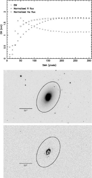
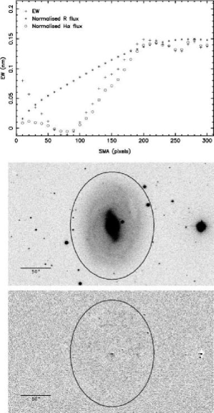
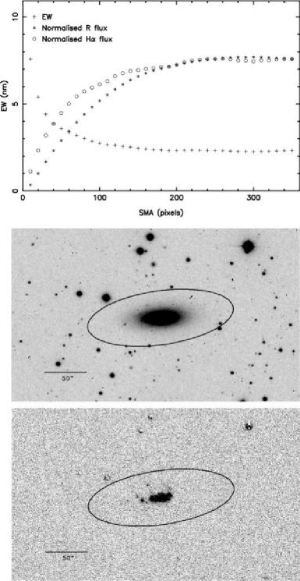
Figure 6: UGC 859, SAB0/a (left); UGC 11238, SB0/a (centre); and UGC 12043, S0/a (right). For each galaxy, the top frame shows the H$\alpha+$[Nii] growth curve (circles), the $R$-band growth curve (asterisks) and the H$\alpha+$[Nii] EW (crosses) as a function of aperture size. The vertical scale relates to the EW plots, and is in nm; the H$\alpha+$[Nii] and $R$-band fluxes are normalised arbitrarily. The horizontal scale is the semi-major axis or radius of the apertures used, in units of 0$\aas@@fstack{\prime\prime}$33 pixels. The images show the $R$-band (central frame) and continuum-subtracted H$\alpha+$[Nii] images (bottom frame), with superposed ellipses to show the apertures used for total line fluxes and $R$ magnitudes.

Figure 6 shows three galaxies classified as extreme early types. Despite their similar classifications and optical appearances, these galaxies show widely differing star formation morphologies. UGC 859 shows strong star formation in a very regular ring, around the edge of the bulge (also described by Pogge & Eskridge pogg (1987)). This is reflected in the EW curve, which exhibits a deep central dip due to the strong continuum from the central bulge, a peak at the radius of the star-forming ring, and a steady drop at larger radii due to the presence of only old stars outside the ring, to an overall value of about 1 nm. This is typical of moderately star-forming bright spiral galaxies. UGC 12043 shows more centrally-concentrated star formation, with just a central peak in the EW curve and a monotonic decline with radius, at least at the resolution of the present data. The overall EW of $\sim$2 nm is high for such an early type galaxy, and both UGC 859 and UGC 12043 are much stronger emission-line sources than were found in the early-type galaxy samples studied by Caldwell et al. (cal91 (1991),cal94 (1994)). UGC 11238, in contrast, has barely detectable line emission, and is included here to highlight the fact that there is no selection bias in favour of star-forming galaxies in the sample, and any statistical analysis will include undetected or barely-detected galaxies like this one. This figure illustrates how well the continuum subtraction removes the light from the old stellar population in the galaxy images.

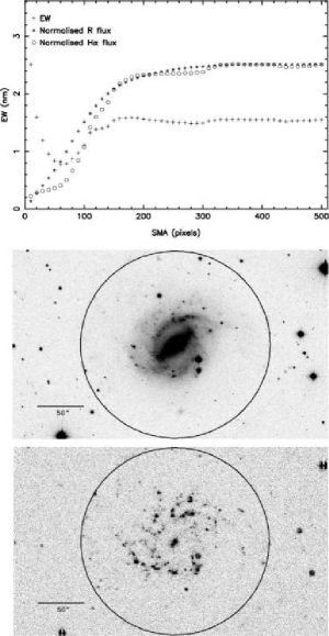
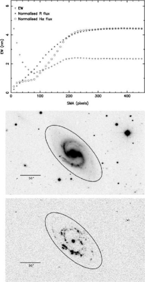
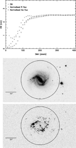
Figure 7: UGC 3685, SBb (left): UGC 4273, SBb (centre); and UGC 6077, SBb (right). See Fig. 6 for details.

The galaxies illustrated in Fig. 7, UGC 3685, UGC 4273 and UGC 6077 are all classified as SBb, and all show qualitatively similar H$\alpha+$[Nii] distributions, with a significant central peak, a star formation ‘desert’ in the region swept out by the bar, and substantial star formation in Hii regions scattered around the disk. This results in an EW curve with a strong central peak, a broad dip, and a gentle outer rise to the plateau level at 1.5–3 nm. The frequency of central peaks in strongly-barred spiral galaxies may reflect the bar-driven feeding of gas into the central regions of galaxies predicted by several authors (e.g., Arsenault arsenau (1989); Quillen et al. quil (1995)). This feeding has been used to explain the high star formation rates generally found in strongly-barred galaxies (e.g., Hawarden et al. hawa (1986); Dressel dres (1988); Huang et al. huan (1996); Martinet & Friedli mart (1997)) via nuclear starbursts.

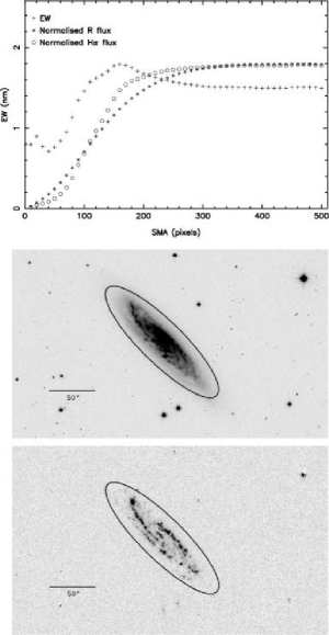
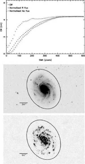
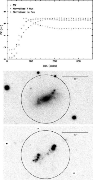
Figure 8: UGC 19, Sbc (left); UGC 6644, Sc (centre); and UGC 3711, IBm (right). See Fig. 6 for details.

Figure 8 shows UGC 19, which is an Sbc with a marked ring of star formation, and is a good example of how this is revealed by a local maximum in the EW at intermediate radii (100-200 pixels semi-major axis, or 4–8 kpc at the adopted distance for this galaxy). UGC 6644, on the other hand, exhibits a monotonically increasing EW curve, showing that the stellar population becomes increasingly dominated by young stars with radius. This is to be expected in the central regions, where the old bulge population is bright in the $R$ band and has little associated line emission, but in UGC 6644 there is evidence that the star formation regions are more widely distributed than the old stellar population even in the disk. This question of the relative distributions of young and old stars, including the effects of inclination on these distributions, will be studied systematically across all Hubble types in a later paper in this series.

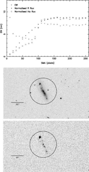
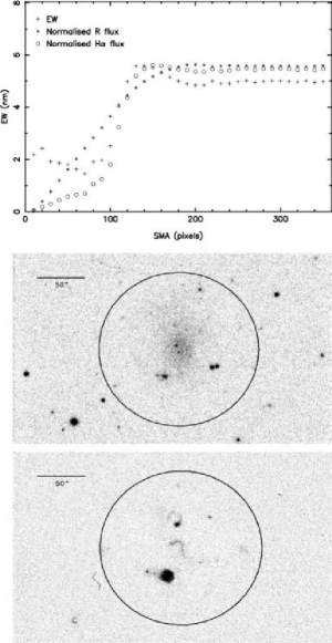
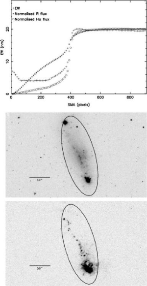
Figure 9: UGC 7326, Im (left); UGC 7866, IABm (centre); and UGC 8098, SBm (right). See Fig. 6 for details.

The sample contains a large number of Magellanic irregular galaxies, and these show an interesting variety in star formation morphologies. UGC 7326 (classified Im), UGC 7866 (an IABm) and UGC 8098 (an SBm, also named NGC 4861; see also Conselice et al. cons (2000) who present ground-based and Hubble Space Telescope imaging of this galaxy) all show highly asymmetric or ‘cometary’ morphologies (Fig. 9) in their continuum-subtracted H$\alpha+$[Nii] images, with extremely intense star formation centres which are displaced very significantly from the centres of the old stellar distributions. This is reflected in long central troughs in the EW curves, with sharp rises to very high values when the star formation centres are reached (all growth curves are centred on the peaks of the old stellar light in the $R$-band images). The decoupling between the smooth old stellar distribution and the highly clumped and asymmetric sites of ongoing star formation is particularly marked in these galaxies. The overall EW values for these three galaxies lie in the range 5–20 nm, much higher than is typical for even late-type spiral galaxies. Local EW values in apertures centred on the Hii complexes lie in the range 50-100 nm for these galaxies. Similarly intense star formation is found in the strongly-barred IBm UGC 3711 (Fig. 8), but in this case the star formation complexes are found in two off-nuclear regions, which appear to be associated with the bar ends.

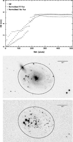
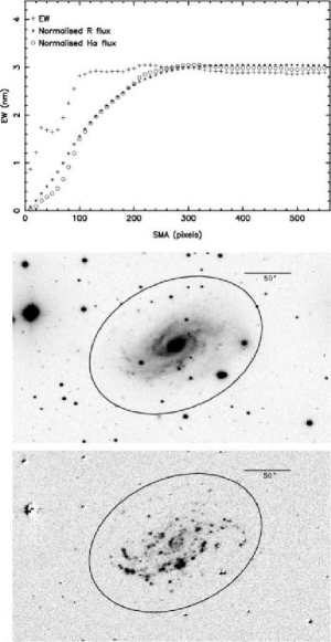
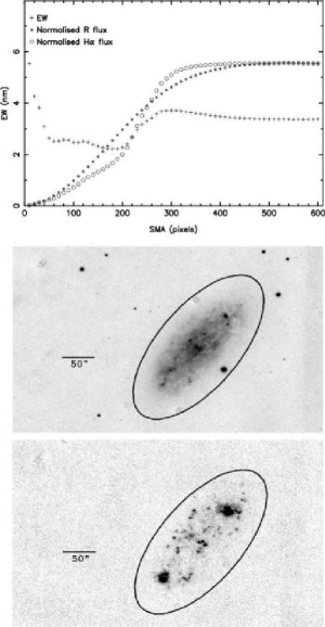
Figure 10: UGC 806, SABcd (left); UGC 3463, SABbc (centre); and UGC 5221, Sc (right). See Fig. 6 for details.

Significant asymmetry in H$\alpha+$[Nii] distributions is also apparent in some of the spiral galaxies. A particularly striking example of this is UGC 806 (Fig. 10), classified SABcd, which contains 3 extremely bright star formation complexes to the east of the bulge. Schaerer et al. (scha (1999)) refer to this object as a Wolf-Rayet galaxy, and note that it may be part of NGC 450 (UGC 806) which appears likely given the close agreement in recession velocity (1693 km s^-1 for the star formation complexes c.f. 1761 km s^-1 systemic). However, even with these three bright regions removed, the Hii region distribution is significantly asymmetric, with a substantial deficit to the north and west. A less marked asymmetry is shown by the SABbc galaxy UGC 3463 (Fig. 10), where most of the bright Hii regions lie south of the nucleus. However, in this case the line of asymmetry coincides with the major axis of this inclined spiral, and it is tempting to ascribe the asymmetry to differential extinction effects, possibly due to systematic offsets between the dust lanes and the star formation centres in spiral arms. The underlying galaxy appears highly symmetric, as shown by the near-IR K-band image of UGC 3463 presented by Peletier et al. (pele (1999)), with no obvious differences between the upper and lower spiral arms in the light emitted by the old stellar population. The question of extinction in arms and asymmetries in H$\alpha$ morphologies will be examined further in a later paper of this series.

UGC 5221 (Fig. 10) is an Sc spiral, possibly in the M81 group, with an unusual star formation morphology in that the bulk of the H$\alpha+$[Nii] emission comes from two regions symmetrically placed along the major axis of the galaxy. If the galaxy elongation is interpreted as an inclined disk (and we note that, for example, Bronkalla & Notni (bron (1990)) cite UGC 5221 as a prime example of a ‘pure-disk’ galaxy), this morphology must be seen as a coincidental alignment, but it does suggest the possibility that the main body of UGC 5221 should be seen as a bar. In this case, the star formation is occurring at the bar ends, as is commonly seen in strongly barred galaxies (e.g., UGC 3711, UGC 4273 and UGC 4708 in this paper).

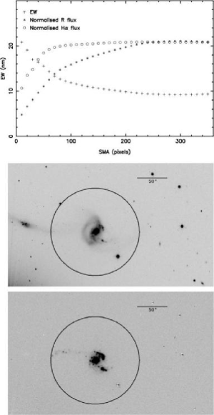
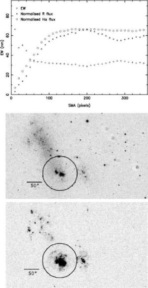
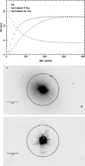
Figure 11: UGC 12699, SBb pec (left); UGC 3847, Irr (centre); and UGC 5398, I0 (right). See Fig. 6 for details.

The sample includes some interacting galaxies, including UGC 12699 (Fig. 11), better known as the prototypical starburst (Weedman et al. weedman (1981)) NGC 7714 or Arp 284. As expected, our data show extremely intense central star formation in NGC 7714, but interestingly none at all from the small companion NGC 7715 (as was also noted by González-Delgado et al. gonz (1995) from their H$\alpha$ imaging), although there are some H$\alpha+$[Nii] knots from the tail apparently joining the two galaxies. This is despite the classification of Im for NGC 7715 and its very disturbed, knotty appearance, which may be due at least in part to foreground stars. Another possible interaction which is worthy of comment is UGC 3847 and UGC 3851 (NGC 2363 and NGC 2366, shown in Fig. 11), both irregular galaxies, with the 2 highest H$\alpha+$[Nii] EWs of all 334 galaxies observed in this study. Drissen et al. (dris (2000)) consider UGC 3847 to be an outlying Hii region of UGC 3851, and note that UGC 3847 is the highest surface brightness Hii region in the entire sky. UGC 3851 is not actually part of the statistical sample, since it is too large to satisfy the selection criteria, but is included in this discussion of individual objects due to its proximity to UGC 3847.

Finally, we include UGC 5398 (Fig. 11) as a cautionary example of the difficulties in interpreting H$\alpha$ emission in a uniform manner. The morphology of the line emission in UGC 5398 is very different to that of most of the sample, showing plumes and possible bubble structures. This galaxy was interpreted by Martin (martin (1998)) as an example of the ‘supershell’ phenomenon, where large numbers of supernovae in a short time interval create large-scale galactic winds, which blow shell structures of this types. However, this morphology is also similar to the Extended Nuclear Emission-line Regions (ENERs) found by Hameed & Devereux (hameed (1999)) in H$\alpha$ imaging of the central regions of early type galaxies, which they ascribe to gas that is either shock-ionized or photoionized by UV radiation from bulge post asymptotic giant branch stars. This, and the likely contribution of AGN line emission from the central regions of at least some of our sample galaxies, are reminders that not all line emission need be related to star formation. These effects will be studied in more detail in later papers in this series.

6.2 Global properties of the sample

The full sample of 334 galaxies provides an excellent database for quantifying star formation activity as a function of galaxy type and luminosity. Some of the most fundamental correlations and distributions are illustrated in the remaining figures in this section.

Figure 12: Distribution of star formation rates as a function of Hubble T type.

Figure 12 shows the distribution of individual galaxy star formation rates as a function of Hubble T-type. The main result from these distributions is that, as expected, spiral galaxies of types Sbc and Sc have the highest individual star formation rates. Barred (SAB and SB types) and unbarred distributions are shown separately, showing that bars appear to be related to moderately higher star formation rates, and the 5 galaxies with the highest star formation rates are all barred. This is not surprising as we have already found that bars can induce circumnuclear star formation (see Fig. 7). For all Hubble types, the modal values of the distributions lie close to zero star formation rate, i.e. very low star formation rates are extremely common for all types.

Figure 13: Mean and median star formation rates as a function of Hubble T type.

Figure 13 shows mean star formation rates (filled points) as a function of Hubble type, with error bars showing the standard error on the mean of the distribution for each type. The open circles show the median star formation rates for each type, to demonstrate that the trends are not dominated by the few outliers at high star formation rates seen in Hubble types Sb–Sc inclusive.

Figures 12 and 13 can be compared directly with the results presented by Kennicutt (k83 (1983)), where we have converted the latter from an assumed Hubble constant of H${}_{0}=$ 50 to our assumed value of 75 km s^-1Mpc^-1. The majority of Kennicutt’s sample (59/97) are of type Sc, and the mean star formation rate for these 59 galaxies is 2.3 M_⊙ yr^-1, with a standard error on the mean of 0.3 M_⊙ yr^-1, in excellent agreement with the value shown in fig. 13. For the 13 Sbc galaxies in Kennicutt’s study, the mean star formation rate is 3.1 M_⊙ yr^-1, standard error 0.4 M_⊙ yr^-1, slightly larger than the mean we find for this type. For the 9 Sb galaxies in Kennicutt’s study, the mean star formation rate is 1.5 M_⊙ yr^-1, standard error 0.3 M_⊙ yr^-1, in excellent agreement with our value. All the other Hubble types have 5 or fewer galaxies in Kennicutt’s study, ruling out a statistically meaningful comparison on a type-by-type basis, but the overall agreement with our fig. 12 is essentially perfect. For example, every one of Kennicutt’s 97 measured star formation rates lies within the range of rates determined in the present study for galaxies of that T-type.

Less good agreement is found with the star formation rates in early-type spirals presented by Caldwell et al. (cal91 (1991), cal94 (1994)). These authors find uniformly low star formation rates in the 5 S0/a galaxies they study (the highest being 0.004 M_⊙ yr^-1, 2 galaxies having measured rates of 0.001 M_⊙ yr^-1 and the remaining 2 upper limits only), while for 6 Sa galaxies the mean rate was found to be 0.17 M_⊙ yr^-1, with a standard error of 0.06 M_⊙ yr^-1 and a maximum of 0.4 M_⊙ yr^-1. For reasons that are not clear, the present study find examples of S0/a and Sa galaxies with much higher star formation rates; for example UGC 859, a type S0/a spiral shown in Fig. 6, has a prominent ring of star formation and a star formation rate of 0.5 M_⊙ yr^-1.

Figure 14: Mean star formation rates as a function of Hubble T type, separated into barred and unbarred types.

Figure 14 again shows mean star formation rates as a function of Hubble type, but this time separated into barred and unbarred types. Again it is clear that bars can enhance star formation, although the effect is only significant in the intermediate Hubble types, and possibly in the extreme late-type galaxies.

Figure 15: Distribution of H$\alpha+$[Nii] EWs as a function of Hubble T type.

Figure 16: Mean and median H$\alpha+$[Nii] EW as a function of Hubble T type.

Equivalent width values provide a measure of star formation efficiency, being normalised by the luminosity of the older stellar population of the galaxy. Figures 15 and 16 show the distribution of individual galaxy H$\alpha$ $+$ [Nii] EWs, and the mean values of this parameter, as a function of Hubble type. It is clear that the highest EWs are seen in the late type spiral galaxies and the irregular galaxies, with the five highest values belonging to Sm or Im galaxies. However, the apparent dependence of mean EW on Hubble type is surprisingly weak for types later than Sbc. It should also be noted that the EW values for the earliest Hubble types may be depressed by the H$\alpha$ absorption from the stars in the dominant bulges in these galaxies.

Figure 15 can be compared with Fig. 3 of Kennicutt (ken98 (1998)), which gives H$\alpha$ $+$ [Nii] EWs for a large sample of nearby spiral galaxies, with the majority of the data being taken from Kennicutt & Kent (ken83 (1983)). For the later-type spirals (Sc–Sm), the agreement in the distributions of EW is good, with marginal evidence for higher EWs in the present sample ($\sim$3.5 nm average over these types, cf. 2.9 nm for the same types in Kennicutt & Kent ken83 (1983)), consistent with the measurement offset noted in the comparison with Kennicutt’s data in section 4.2. However, for the earliest types (S0/a–Sab), the agreement is less good, with the present sample containing several early-type galaxies with H$\alpha$ $+$ [Nii] EWs several times larger than those found in Kennicutt’s compilation. This is most marked for the S0/a type galaxies, where all 11 of Kennicutt’s galaxies lie well below 0.5 nm EW, compared to a mean of 1.7 nm for the 16 galaxies in the present sample. Even for the Sb type galaxies, the present study finds a mean EW approximately twice that of Kennicutt (ken98 (1998)). Apart from this discrepancy, the overall pattern of EW with increasing T-type is very similar in the two studies, with Kennicutt (ken98 (1998)) also finding mean EW to increase from type S0/a to type Sc, and then to remain approximately constant for the later types.

Loveday et al. (love99 (1999)) present histograms of H$\alpha$ EW for large numbers of galaxies from the Stromlo-APM redshift survey. Since their data are spectroscopic with a resolution of $\sim$5Å, they have resolved the H$\alpha$ and [Nii] lines and present EWs for H$\alpha$ only. Over all spiral types, their median H$\alpha$ EW is 1.06 nm, and for irregulars it is 1.69 nm. These values are significantly lower than those for both the present study and Kennicutt (k83 (1983)). The median H$\alpha$ $+$ [Nii] EWs for the present study are 2.80 nm for spirals and 3.75 nm for irregulars, which reduce to 2.2 and 3.5 nm respectively after application of the standard Kennicutt correction for [Nii] contamination, still approximately double the EW values found by Loveday et al. (love99 (1999)). The median H$\alpha$ $+$ [Nii] EWs for the 114 spirals observed by Kennicutt (k83 (1983)), and for the 110 spirals observed by Romanishin (rom90 (1990)), are both 2.4 nm, or 1.8 nm after correction for [Nii] emission. The reasons for the lower values found by Loveday et al. (love99 (1999)) are not clear at present, but seem unlikely to be due entirely to differences in galaxy classifications, since all types later than Sab in the present study have median EW values higher than the overall mean found by Loveday et al. (love99 (1999)). Other factors that may play a part are different surface brightness selection criteria between the APM survey and the nearby galaxy catalogues used by the other studies, and possibly aperture effects, although all of these studies present EWs which should be close to total values.

Figure 17: Log H$\alpha+$[Nii] EW as a function of total $R$-band absolute magnitude. The dashed line shows the EW completeness limit of 0.4 nm.

Figure 17 shows the distribution of individual galaxy H$\alpha$ $+$ [Nii] EWs, where the decimal logarithm is plotted to better show separate points, as a function of total $R$ magnitude. This again shows a surprising lack of dependence of EW on the properties of the underlying galaxy. The diagram mainly shows a large scatter in EW at any given luminosity. Any trend in EW with luminosity is due to a population of very low EW galaxies seen in the brightest spiral galaxies only (and these are the galaxies most likely to have EWs reduced by H$\alpha$ absorption), but apart from this the distribution is completely flat as a function of luminosity. This lack of correlation has been found by previous studies, but over a smaller range in absolute magnitude. For example, Kennicutt & Kent (ken83 (1983)) find no luminosity dependence in the H$\alpha$ $+$ [Nii] EW of Sc spirals over a 5 mag range in M_B. Tresse and Maddox (tres98 (1998)) find no correlation in an identical plot for 138 galaxies out to $z=$0.3 from the Canada-France Redshift Survey (CFRS), over a 6 mag range in M_B. However, Tresse et al. (tres02 (2002)) do find a trend in the closely related parameter, Log(L(H$\alpha$)/L_B), when plotted against M_B, for CFRS galaxies between redshift 0 and 1.1. This trend is in the sense that the most luminous galaxies have higher H$\alpha$-to-continuum flux ratios than the lower luminosity galaxies, although the strength of the correlation depends on the reddening correction applied, and the interpretation of this result is complicated by the fact that the most luminous galaxies also tend to be the most distant.

An alternative way to prevent size effects from masking trends in star formation rate is to normalise by galaxy surface area, giving an H$\alpha+$[Nii] surface brightness, or equivalently a star formation rate per unit surface area. Figures 18 and 19 present such data for the present galaxy sample, where the surface brightness used is a hybrid value, plotted in arbitrary units. This hybrid surface brightness is based on the total detected H$\alpha+$[Nii] flux, divided by the square of the $R$-band Petrosian radius of the galaxy. This latter radius is defined to be independent of galaxy distance and photometric errors, and is basically the radius at which the local surface brightness is a given factor lower than the mean surface brightness within that radius. We adopt the definition of Petrosian radius used by Shimasaku et al. (shim (2001)), who adopt a value of 0.2 for the $\eta$ parameter used to define the Petrosian radius (see Petrosian petr (1976) for the original explanation of this parameter). This radius is much better defined for the smooth $R$-band profiles than for the H$\alpha+$[Nii] images, hence the use of the hybrid surface brightnesses. Figure 18 shows the distributions of this surface brightness parameter as a function of galaxy Hubble type, showing that the distributions are essentially independent of galaxy type, although the range in surface brightness is broad at all Hubble types. In particular, it is noteworthy that the irregular galaxies (T$=$10) have a very similar distribution to the spiral galaxies, even though their overall star formation rates are much lower.

This conclusion is emphasised by Fig. 19, which shows H$\alpha+$[Nii] surface brightness as a function of total $R$-band galaxy magnitude. Again the distribution is essentially flat, with the only obvious outliers being two bright spiral galaxies with high H$\alpha+$[Nii] surface brightnesses.

Figure 18: H$\alpha+$[Nii] surface brightness as a function of galaxy type.

Figure 19: H$\alpha+$[Nii] surface brightness as a function of total $R$-band absolute magnitude.

7 Conclusions and future work

We have presented new narrow-band H$\alpha+$[Nii] line and $R$-band imaging data photometry, of a sample of 334 galaxies carefully selected to span all star-forming types in the local Universe. The galaxies were taken from the UGC, and hence are subject to the selection criteria of that catalogue, and in addition we have required a measured recession velocity less than 3000 km s^-1, D₂₅ diameters between 1$\aas@@fstack{\prime}$7 and 6$\aas@@fstack{\prime}$0, and Hubble types between S0/a and Im.

The new data have been used to quantify the distributions of star formation activity as a function of galaxy type and luminosity. We find a strong correlation between galaxy Hubble type and total star formation rate, in the expected sense that the most strongly star-forming galaxies are those of Hubble types Sbc and Sc, although even within these types there is a wide range in star formation rates. H$\alpha+$[Nii] EW values, averaged over entire galaxies, give a measure of star formation activity normalised by the stellar luminosity of the galaxy; these also show a trend with galaxy type, with early-type spiral galaxies having low EW values, and irregular galaxies the highest EWs, at least in the mean. However, the distribution of EW as a function of galaxy luminosity is surprisingly flat, both in terms of median EW and the scatter in this parameter.

In this paper we have only skimmed the surface of the science to be undertaken in this project. A key area for further study concerns the corrections which need to be applied to H$\alpha$ fluxes derived from narrow-band imaging to account for [Nii] line contamination and extinction internal to the galaxies under study, since these dominate the uncertainties in the derived star formation rates (see also the detailed examination of this question by Charlot et al. char02 (2002), and work by Buat et al. buat02 (2002) and Rosa-González et al. gonz02 (2002)). The spatial dependence of the [Nii] correction will be investigated, since the [Nii] line strength depends on metallicity and requires a harder radiation field than H$\alpha$, suggesting that the relative strengths of the two lines may be very different in the disk and circumnuclear environments. We will also look at the type dependence of the H$\alpha$ extinction correction in detail, building on the work of Kennicutt & Kent (ken83 (1983)), since our sample contains many late-type and low-luminosity galaxies which were not well represented in their study.

Sect. 6.1 of the present paper illustrates that the H$\alpha$ images contain substantial information on the distribution of line-emitting gas within galaxies, as well as on the total quantity. We will use this information to compare the distributions of star formation regions with the old stellar populations (as represented by $R$-band light) in galaxy disks and in irregular galaxies, with a key question being whether new stars are produced with a distribution similar to that of the old stars, or whether there is any evidence for disks and irregular galaxies being constructed ‘inside-out’ or ‘outside-in’. The distributions of both new and old stellar populations will be quantified for this analysis by concentration indices.

Whilst the present H$\alpha$ sample has been constructed to sample the field population, i.e. avoiding the centres of rich galaxy clusters, it still samples a range of galaxy environments, including completely isolated galaxies, galaxies in known pairs or groups, and some interacting systems. We will thus study the effects of environment (local galaxy density) and interactions with very close neighbours on star formation rate, surface density and distribution in spiral and irregular galaxies, for comparison with results obtained by Kennicutt et al. (ken87 (1987)), Loveday et al. (love99 (1999)), Carter et al. (cart01 (2001)) and Koopman et al. (koopman (2001)).

A final aim for this study is to determine the total star formation rate in the local Universe, by correcting the observed galaxy sample for the known selection effects to represent a volume-limited sample. This will yield a galaxy luminosity function, from which we can estimate the total star formation rate per unit volume of the local Universe, and the contribution to this total from different galaxy luminosities and Hubble types. We believe this to be a complementary approach to previous studies in this area, e.g. those by Gallego et al. (gallego95 (1995)) who looked at 176 star-forming galaxies out to $z\sim$0.045, and Tresse & Maddox (tres98 (1998)), 138 galaxies to $z\sim$0.3. Our study is much more local than these, raising concerns about how representative a volume it may sample, but intensively samples that volume given the large sample size. The proximity of the galaxies also enables us to include the faintest star-forming dwarfs, and gives us excellent spatial resolution within the galaxies, thus disentangling nuclear and disc contributions to the total star formation rate.

- (1) Arsenault, R. 1989, A&A, 217, 66
- (2) Bell, E.F., & Kennicutt, R.C. 2001, ApJ, 548, 681
- (3) Bronkalla, W., & Notni, P. 1990, AGAb, 5, 85
- (4) Buat, V., Boselli, A., Gavazzi, G., Bonfanti, C. 2002, A&A, 383, 801
- (5) Caldwell, N., Kennicutt, R.C., Phillips, A.C., & Schommer, R.A. 1991, ApJ, 370, 526
- (6) Caldwell, N., Kennicutt, R.C. & Schommer, R.A. 1994, AJ, 108, 1186
- (7) Cardelli, J.A., Clayton, G.C., & Mathis, J.S. 1989, ApJ, 345, 245
- (8) Carter, B.J., Fabricant, D. G., Geller, M. J., Kurtz, M. J., McLean, B. 2001, ApJ, 559, 606
- (9) Charlot, S., Kauffman, G., Longhetti, M., Tresse, L., White, S.D.M., Maddox, S.J., & Fall, S.M. 2002, MNRAS, 330, 876
- (10) Condon, J.J. 1992, ARAA, 30, 575
- (11) Conselice, C.J., Gallagher, J.S., Calzetti, D., Homeier, N., & Kinney, A. 2000, AJ, 119, 79
- (12) Cram, L., Hopkins, A., Mobasher, B., & Rowan-Robinson, M. 1998, ApJ, 507, 155
- (13) Dopita, M.A., & Ryder, S.D. 1994, ApJ, 430, 163
- (14) Dressel, L.L. 1988, ApJ, 329, L69
- (15) Drissen, L., Roy, J.R., Robert, C., Devost, D., Doyon, R., 2000, AJ, 119, 688
- (16) Gallagher, J.S., Hunter, D.A., & Tutukov, A.V. 1984, ApJ, 284, 544
- (17) Gallego, J., Zamorano, J., Aragón-Salamanca, A., & Rego, M. 1995, ApJ, 455, L1
- (18) Gallego, J., Zamorano, J., Rego, M., Alonso, O., & Vitores, A.G. 1996, A&AS, 120, 323
- (19) González-Delgado, R. M., Perez, E., Diaz, A., et al. 1995, ApJ, 439, 604
- (20) Hameed, S., & Devereux, N. 1999, AJ, 118, 730
- (21) Hawarden, T.G., Mountain, C.M., Leggett, S.K., & Puxley, P.J. 1986, MNRAS, 221, 41P
- (22) Hopkins, A.M., Connolly, A.J., & Szalay, A.S. 2000, AJ, 120, 2843
- (23) Huang, J.H., Gu, Q.S., Hawarden, T.G., Liao, X.H., & Wu, G.X. 1996, A&A, 313, 13
- (24) James, P.A., Shane, N.S., Knapen, J.H., Etherton, J., & Percival, S.M. 2003, in preparation
- (25) Kennicutt, R.C. 1983, ApJ, 272, 54
- (26) Kennicutt, R.C., & Kent, S.M. 1983, AJ, 88, 1094
- (27) Kennicutt, R.C., Keel, W.C., van der Hulst, J.M., Hummel, E., & Roettiger, K.A. 1987, AJ, 93, 1011
- (28) Kennicutt, R.C. 1992, ApJ, 388, 310
- (29) Kennicutt, R.C., Tamblyn, P., & Congdon, C.W. 1994, ApJ, 435, 22
- (30) Kennicutt, R.C. 1998, ARA&A, 36, 189
- (31) Koopman, R.A., Kenney, J.D.P., & Young, J. 2001, ApJS, 135, 125
- (32) Landolt, A.U. 1992, AJ, 104, 340
- (33) Lanzetta, K.M., Yahata, N., Pascarelle, S., Chen, H.-W., & Fernández-Soto, A. 2002, ApJ, 570, L492
- (34) Lehnert, M.D., & Heckman, T.M. 1996, ApJ, 472, 546
- (35) Loveday, J., Tresse, L., & Maddox, S. 1999, MNRAS, 310, 281
- (36) Madau, P., Ferguson, H. C., Dickinson, et al. 1996, MNRAS, 283, 1388
- (37) Madau, P., Pozetti, L., & Dickinson, M. E. 1998, ApJ, 498, 106
- (38) Martin, C.L. 1998, ApJ, 506, 222
- (39) Martinet, L., & Friedli, D. 1997, A&A, 323, 363
- (40) Niklas, S., Klein, U., & Wielebinski, R. 1997, A&A, 322, 19
- (41) Nilson, P. 1973, Uppsala general catalogue of galaxies, Uppsala Obs. Ann., vol. 6 (UGC)
- (42) Peletier, R. F., Knapen, J. H., Shlosman, I., et al. 1999, ApJS, 125, 363
- (43) Petrosian, V. 1976, ApJ, 209, L1
- (44) Pogge, R.W., & Eskridge, P.B. 1987, AJ, 93, 29
- (45) Quillen, A.C., Frogel, J.A., Kenney, J.D.P., Pogge, R.W., & Depoy, D.L. 1995, ApJ, 441, 549
- (46) Romanishin, W. 1990, AJ, 100, 373
- (47) Rosa-González, D., Terlevich, E., Terlevich, R. 2002, MNRAS, 332,283
- (48) Ryder, S.D., & Dopita, M.A. 1993, ApJS, 88, 415
- (49) Ryder, S.D., & Dopita, M.A. 1994, ApJ, 430, 142
- (50) Salpeter, E.E. 1955, ApJ, 121, 161
- (51) Schaerer, D., Contini, T., & Pindao, M. 1999, A&AS, 136, 35
- (52) Schechter, P.L. 1980, AJ, 85, 801
- (53) Schlegel, D.J., Finkbeiner, D.P., & Davis, M. 1998, ApJ, 500, 525
- (54) Shane, N.S. 2002, PhD thesis, Liverpool John Moores University.
- (55) Shimasaku K., et al. 2001, AJ, 122, 1238
- (56) Steidel, C.C., Adelberger, K.L., Giavalisco, M., Dickinson, M., & Pettini, M. 1999, ApJ, 519, 1
- (57) Tresse, L., & Maddox, S.J. 1998, ApJ, 495, 697
- (58) Tresse, L., Maddox, S., Loveday, J., & Singleton, C. 1999, MNRAS, 310, 262
- (59) Tresse, L., Maddox, S.J., Le Fèvre, O., & Cuby, J.-G. 2002, MNRAS, 337, 369
- (60) Tully, R.B. 1988, Nearby Galaxies Catalogue (Cambridge: Cambridge Univ. Press)
- (61) Weedman, D. W., Feldman, F. R., Balzano, V. A., et al. 1981, ApJ, 248, 105
- (62) Young, J.S., Allen, L., Kenney, J.D.P., Lesser, A., & Rownd, B. 1996, AJ, 112, 1903
- (63)