On Solar Radius Variation with magnetic Activity

Abstract

In response to the claim by Dziembowski et al. (2001) that the solar radius decreases with magnetic activity at the rate of 1.5 km yr^-1, we consider the theoretical question whether a radius variation is expected with the solar cycle. If the radius variation is caused by the magnetic pressure of toroidal flux tubes at the bottom of the convection zone, then the dynamo model of Nandy and Choudhuri (2002) would suggest a radius decrease with magnetic activity, in contrast to other dynamo models which would suggest a radius increase. However, the radius decrease is estimated to be only of the order of hundreds of metres.

1 Introduction

By analyzing the f-mode frequency data from MDI for the period 1996–2001, Dziembowski et al. (2001) claimed that the Sun shrinks in radius from the solar minimum to the solar maximum, at the rate of about 1.5 km per year. If correct, then this will certainly be a most dramatic discovery in solar physics. However, this claim has not yet been supported by other researchers, who often present conflicting results. Antia (2003) provides a review of the subject and concludes that there is no compelling evidence for solar radius change. It may be noted that some earlier studies (Nöel, 1997; Emilio et al., 2000) reported much larger radius variation (up to 700 km) based on other (non-helioseismic) methods. It is clear that more work is needed before a definitive conclusion can be reached. The aim of this paper is to discuss whether on theoretical grounds we expect a solar radius variation with solar cycle. Other than some early work by Spruit (1982, 1994), we have not been able to find any other theoretical analysis of this problem. In the light of recent developments of solar physics, this theoretical question certainly needs revisiting.

There are two ways in which a magnetic field present in the solar interior may lead to an increase of solar radius.

1. The pressure of the magnetic field embedded in the gas may cause the gas to expand, thereby inflating the size of the Sun.

2. The inhibition of convection by the magnetic field may cause a piling up of heat below the magnetic field. This would result in heating of the surrounding regions, leading to an expansion.

From both of these arguments, it appears that the radius of the Sun should increase when more magnetic fields are present. Since we normally think of the solar maximum as being the time when the Sun has more magnetic fields in the interior, we would expect the Sun to be larger in size during the solar maximum. Shrinking of the Sun with increasing magnetic activity, therefore, would seem improbable at the first sight.

We shall argue that the recent solar dynamo model of Nandy and Choudhuri (2002), in principle, allows for the possibility of shrinking of the Sun during the solar maximum. The important theoretical question is whether the theoretically expected radius decrease agrees with the claim of Dziembowski et al. (2001). Spruit (1982, 1994) studied the effect of heat blocking by magnetic fields and concluded that the total radius variation cannot be more than 0.14 km. We mainly look at the other effect of magnetic pressure and present order-of-magnitude estimates, suggesting that the radius variation, for reasonable assumptions, cannot be as large as what Dziembowski et al. (2001). We have also made a mathematical formulation of the problem, to go beyond order-of-magnitude estimates. To our surprise, we found that the mathematical problem is much more difficult to solve than what we anticipated. Although our mathematical analysis so far has not yielded very definite results, we present a brief account of it to help future researchers who may wish to analyze this problem in greater depth.

Section 2 addresses the question whether we expect the radius to increase or decrease during the solar maximum. An order-of-magnitude estimate is presented in Section 3, showing that a much smaller variation of radius is expected than what is reported by Dziembowski et al.  (2001). Our incomplete mathematical analysis is given in Section 4. Finally, our conclusions are summarized in Section 5.

2 Increase or decrease of radius with magnetic activity?

Both the effects listed above—expansion due to magnetic pressure and heat blocking by inhibition of convection—would lead to an increase of the solar radius when there is more magnetic flux. So it appears that the Sun can shrink with increasing magnetic activity only if there is less magnetic flux inside the Sun at the time of solar maximum. We know that the Sun has much more magnetic flux near the surface in the form of sunspots during the solar maximum. It used to be tacitly assumed that the magnetic flux in the interior of the Sun should also have a peak during the solar maximum. Some recent dynamo models, however, raise doubts about this assumption.

It has been realized for some time that the meridional circulation plays an important role in the solar dynamo (Choudhuri et al.,  1995). This meridional circulation is poleward near the surface and must be equatorward at the bottom of the solar convection zone (SCZ). With the mapping of angular velocity distribution in the solar interior by helioseismology, it is clear that the strongest gradient of angular velocity occurs at high latitudes within the tachocline and that is the most likely region for the creation of toroidal field. To explain why active regions appear at low latitudes, Nandy and Choudhuri (2002) have developed a solar dynamo model in which the meridional flow penetrates a little bit below the tachocline and advects the strong toroidal field (created at high latitudes inside the tachocline) to low latitudes through convectively stable layers below the tachocline. Only when the meridional circulation rises in the low latitudes, the toroidal fields are brought within the SCZ and rise quickly due to magnetic buoyancy to form sunspots. In the model of Nandy and Choudhuri (2002), therefore, the toroidal flux which erupts at the solar surface was created a few years earlier at high latitudes within the tachocline, since it took time for the flux to be transported from there. If the meridional flow speed at the base of the SCZ is taken to be of order 1.2 m s^-1 (Hathaway et al., 2003), then the time taken for flux transport should be in the range 5-10 yr. Hence the flux should have been created a few years before the solar maximum. In this scenario, the solar maximum is the time when the Sun merely gets rid of the flux stored below the SCZ. In contrast to the traditional dynamo models in which during the solar maximum the Sun generates the strong toroidal field and the interior flux has a peak value, the model of Nandy and Choudhuri (2002) suggests the solar maximum to be the time when the magnetic flux in the Sun is reduced after being created a few years earlier. Although the solar maximum is the period when the magnetic flux near the surface in the form of sunspots peaks, it may also be a time when the magnetic flux at the bottom of the SCZ actually decreases. So, to settle the question whether a magnetic effect would lead to increase of decrease of the solar radius, we need to ascertain whether the magnetic effect is caused by the magnetic flux near the surface or the magnetic flux at the bottom of the SCZ. We point out that several simulations of active region formation (Choudhuri and Gilman, 1987; Choudhuri, 1989; D’Silva and Choudhuri, 1993; Fan et al.,  1993; D’Silva and Howard, 1993; Caligari et al.,  1995) have pinned down the value of the magnetic field at the bottom of SCZ to be around $10^{5}$ G.

We first make a few remarks on Spruit’s analysis of the heat blocking problem (Spruit, 1982, 1994). If the magnetic field is sufficiently strong to suppress convection, the effects of heat blocking become independent of the magnetic field (i.e. it does not matter if the magnetic is just strong enough to suppress the convection or much stronger than that). On the other hand, results of radius variation due to magnetic pressure depend critically on the value of the magnetic field, as we shall see below. Spruit (1982) mainly considered heat blocking by vertical flux tubes near the solar surface. Although we believe in the existence of strong toroidal flux tubes with $10^{5}$ G magnetic field at the bottom of SCZ, heat blocking by these flux tubes will not have much effect for two reasons. Firstly, due to the high concentration of magnetic field inside these flux tubes, the flux tubes would occupy a smaller volume compared to the volumes of flux tubes below the sunspots. Hence convection would be suppressed in much smaller volumes. Secondly, the bottom of the SCZ is the region where convective heat transport just begins to win over the radiative transport. A suppression of convection there is not expected to have as much effect as it would have in the interior of SCZ. We thus conclude that we can still trust Spruit’s results and his conclusion that the radius variation can at most be of order $2\times 10^{-7}R_{\odot}$, which is only $0.14$ km. It is not only considerably less than what is reported by Dziembowski et al.  (2001), it also has the wrong sign. More heat blocking below sunspots takes place during the solar maximum and the radius should increase at that time.

If magnetic flux decreases at the bottom of SCZ during the solar maximum, as suggested by the model of Nandy and Choudhuri (2002), then the magnetic pressure is reduced and it is possible that the Sun shrinks due to this at the time of the solar maximum. We now turn to making an estimate of how much this radius decrease is expected to be.

3 Basic considerations and rough estimates

We now consider radius variations due to magnetic pressure of the concentrated flux tubes at the bottom of SCZ. When the magnetic flux is created, it disturbs the hydrostatic equilibrium. It is well known that the time scale for restoration of hydrostatic equilibrium is very short (see, for example, Schwarzschild, 1958, p. 32). As Schwarzschild (1958) comments: “There is no doubt that punishment would follow swiftly for any disobedience of the hydrostatic law.” We, therefore, assume that the Sun would fairly quickly adjust itself to a new hydrostatic equilibrium when the magnetic field is created. So we shall basically compare hydrostatic equilibria with and without magnetic fields embedded inside, without bothering about the adjustment time scales. Our approach thus is going to be quite different from the approach of Spruit (1982) while studying the heat blocking problem, in which two time scales (the diffusion time and the Kelvin-Helmholtz time) play important roles.

To calculate the expansion of a flux tube due to magnetic pressure, we need to specify the thermodynamic conditions. If the temperature in the interior of the flux tube is the same as the outside temperature, then certainly the flux tube expands due to magnetic pressure (see, for example, Choudhuri, 1998, §14.7). However, such a flux tube also tends to be buoyant and to rise against gravity. The flux tubes are believed to be stored in the mildly sub-adiabatic region immediately below the bottom of the SCZ. If a buoyant flux tube rises in a region of sub-adiabatic temperature gradient, it can be easily shown that it becomes less buoyant (Parker, 1979, §8.8; Moreno-Insertis, 1983). One expects that the flux tube would rise until it becomes neutrally buoyant, i.e. until the interior temperature decreases sufficiently to make the density inside and outside exactly equal. If the flux tube is neutrally buoyant, then its density is no different from the outside density and there is no increase in the overall size of the system. Thus, if all the magnetic flux inside the Sun remained neutrally buoyant, then there would be no change in the solar radius at all. In view of our lack of understanding of the physics of flux tubes at the bottom of SCZ, let us allow for the possibility that this may not be the case. The penetrating meridional circulation proposed in the model of Nandy and Choudhuri (2002) would drag the flux tubes downward, making them hotter and not allowing them to come up by magnetic buoyancy. Considering a favourable circumstance that the flux tubes are not colder than the surroundings, let us see if we can have sufficient radius increase of the Sun.

We now make a rough estimate by considering a one-dimensional atmosphere in rectangular geometry. Suppose a horizontal magnetic field $B$ is created within this atmosphere in a layer between $z$ and $z+L$. Because of the magnetic pressure inside this layer, the gas pressure would be less than the pressure $p$ that would exist there if the magnetic field were not present. To find the corresponding density decrease, we assume the region with the magnetic field to have the same temperature as the surrounding region. Then we can give the same arguments which we give for flux tubes in thermal equilibrium with surroundings (see, for example, Choudhuri, 1998, §14.7) and conclude that the density decrease is given by

$$\frac{\delta\rho}{\rho}\approx\frac{B^{2}}{8\pi p}.$$

In a one-dimensional atmosphere, such a density decrease implies that the magnetic layer would be inflated by an amount $\delta L$ compared to thickness which the gas in this layer would have in the absence of the magnetic field. Hence, when the magnetic field is created, the overlying atmosphere will be pushed up by this amount $\delta L$, which is given by

$$\frac{\delta L}{L}\approx\frac{\delta\rho}{\rho}.$$

Note that we are not bothering about the signs of $\delta\rho$ and $\delta L$. Then from (1),

$$\frac{\delta L}{L}\approx\frac{B^{2}}{8\pi p}.$$

Since

$$F=BL$$

is the magnetic flux through the magnetic layer (per unit length of the layer measured in a direction perpendicular to $B$ in the layer), we can write (2) as

$$\delta L\approx\frac{F^{2}}{8\pi pL}.$$

It is clear from (3) that the rise of the atmosphere is more if the same flux $F$ is concentrated in a narrower layer (i.e. if the magnetic field is stronger).

Taking $p=5\times 10^{13}$ dyn cm^-2 at the bottom of the SCZ, (2) tells us that for magnetic field created there we must have

$$\delta L\approx 7.7\times 10^{-6}\left(\frac{B}{10^{5}}\right)^{2}L.$$

For magnetic field of order $10^{5}$ G, we expect $\delta L/L$ to be only of order $10^{-5}$.

We now estimate the radius shrinkage of the Sun due to the release of magnetic flux from the interior during the solar maximum. Assume that there are about $10^{4}$ eruptions during the maximum and each eruption brings out flux in the range from $10^{20}$ Mx to $10^{21}$ Mx. Then the total flux coming out of the interior of the Sun is about $10^{24}$ – $10^{25}$ Mx. This flux comes from the bottom of SCZ, where the magnetic field is $10^{5}$ G. This gives a cross-sectional area of $10^{19}$ – $10^{20}$ cm². To compare with the one-dimensional model, we distribute this flux in a uniform shell at the bottom of SCZ. Taking $L$ to be the thickness of this shell, the cross-sectional area through which the magnetic field passes should be equal to $\pi R_{\rm bot}L$, where $R_{\rm bot}$ is the radial distance of the bottom of SCZ. Equating this cross-sectional area to $10^{19}$ – $10^{20}$ cm², we get $L$ in the range from about $10^{8}$ cm to $10^{9}$ cm (i.e. from about 1000 km to 10,000 km). It follows from (4) that the expected maximum shrinkage of the Sun can only be in the range from 0.1 km to 1 km. If this radius shrinkage takes place over 5 years, then even the most favourable value 1 km of radius shrinkage will give a shrinkage rate of only 0.2 km per year. According to (3), the magnetic field at the bottom of SCZ has to be squeezed in a layer narrower by one order of magnitude if the radius shrinkage rate had to be as large as what Dziembowski et al. (2001) find. This would imply the horizontal magnetic field at the bottom of SCZ should be of order $10^{6}$ G. Such a strong field would create problems with the theoretical explanation of Joy’s law (D’Silva and Choudhuri 1993).

It should be kept in mind that the radius shrinkage rate estimated above is an over-estimate. If the magnetic flux tends to become neutrally buoyant in some regions, then certainly the radius variation will be less. Additionally, Choudhuri (2003) has argued that magnetic flux would exist in concentrated form only in limited regions at the bottom of SCZ, the field being more diffuse in other regions. Since diffuse magnetic field would not cause much radius variation, in accordance with (3), the actual radius variation would be smaller if concentrated magnetic field regions are intermittent.

4 A hydrostatic model with a magnetic layer

After the order-of-magnitude estimate, we now try to construct hydrostatic models of the SCZ, with and without magnetic fields in the interior, to determine the distance by which the outer surface shifts between these two models. After considering a hydrostatic model without magnetic fields, we shall assume that the magnetic field is created in a shell $r_{b}<r<r_{t}$ and calculate the new equilibrium. To our great surprise, we found this problem to be much more complicated than what we expected. Although we have not been able obtain very definite results, we discuss the formulation of the problem to provide guidance for future researchers who may wish to tackle the problem with more realistic models.

Let us first consider the case without the magnetic field and construct a hydrostatic model from the bottom of the overshoot layer at $R_{BCZ}=0.67R_{\odot}$ to the surface at $R_{\odot}$. Let $p_{0}(r),\rho_{0}(r),T_{0}(r)$ be the pressure, density and temperature structures in this case. The equation for hydrostatic equilibrium is given by

$$\frac{d{p_{0}(r)}}{d{r}}=-\frac{\rho_{0}(r)GM_{\odot}}{r^{2}}.$$ (5)

The temperature gradient is slightly sub-adiabatic in the overshoot layer and slightly super-adiabatic in the SCZ. We assume an adiabatic stratification throughout and use the equation of state

$$p_{0}(r)=\kappa{\rho_{0}(r)}^{\gamma}.$$ (6)

Substituting (6) in (5) and solving the resulting ODE with the boundary condition $\rho_{0}(R_{\odot})=0$, we have the following expressions for $\rho_{0}(r),p_{0}(r)$, and $T_{0}(r)$. To compute the temperature we have used the ideal gas law $p=\rho R_{gas}T$.

$$\begin{pmatrix}\rho_{0}(r)\\ p_{0}(r)\\ T_{0}(r)\\ \end{pmatrix}=\begin{pmatrix}[\frac{\gamma-1}{\gamma}\frac{GM}{\kappa}\{\frac{1}{r}-\frac{1}{R_{\odot}}\}]^{\frac{1}{\gamma-1}}\\ \kappa[\frac{\gamma-1}{\gamma}\frac{GM}{\kappa}\{\frac{1}{r}-\frac{1}{R_{\odot}}\}]^{\frac{\gamma}{\gamma-1}}\\ \frac{\gamma-1}{\gamma}GM\{\frac{1}{r}-\frac{1}{R_{\odot}}\}\\ \end{pmatrix}$$ (7)

We now consider that a magnetic field $B(r)$ is created in the shell $r_{b}<r<r_{t}$, i.e. the magnetic field remains zero in the layers below and above. The hydrostatic equation is satisfied piecewise in all the three layers. The subscript ’$1$’ indicates quantities below the magnetic shell, the subscript ’$2$’ denotes quantities inside the magnetic layer, whereas ’$3$’ indicates those above. In the field-free regions ’1’ and ’3’, pressure and density should satisfy the hydrostatic equation (5) and the adiabatic equation (6) (with the subscripts ’1’ and ’3’ replacing the subscript ’0’). Then the solutions also will be similar to (7). We can assume the layer below to remain unchanged after the introduction of the magnetic field. So $\rho_{1}(r)$, $p_{1}(r)$ and $T_{1}(r)$ are equal to $\rho_{0}(r)$, $p_{0}(r)$ and $T_{0}(r)$ below $r=r_{b}$. In the case of the upper layer, we assume that outer radius is now $R$ instead of $R_{\odot}$. So $\rho_{3}(r)$, $p_{3}(r)$ and $T_{3}(r)$ can simply be obtained from (7) by replacing $R_{\odot}$ by $R$ (which essentially means changing the constant of integration), i.e.

$$\rho_{3}(r)=\Big{[}\frac{(\gamma-1)GM_{\odot}}{\gamma\kappa}\Big{(}\frac{1}{r}-\frac{1}{R}\Big{)}\Big{]}^{\frac{1}{\gamma-1}}$$ (8)

with similar corresponding expressions for $p_{3}(r)$ and $T_{3}(r)$.

Let us now focus our attention in the magnetic layer $r_{b}<r<r_{t}$. The hydrostatic equation there is

$$\frac{d}{d{r}}\left[p_{2}(r)+\frac{B^{2}(r)}{8\pi}\right]=-\frac{\rho_{2}(r)GM_{\odot}}{r^{2}}.$$ (9)

Actually, there should also be a magnetic tension term which would break the spherical symmetry. Apart from breaking the spherical symmetry, the other problem which such a term introduces is that it cannot be balanced by a combination of gradient forces, like the pressure gradient and gravity (which comes from the gradient of gravitational potential). For flux tubes at the bottom of SCZ, the magnetic tension term is supposed to be negligible compared to other term (the gradient of magnetic pressure becomes much larger near the boundaries of flux tubes). Hence we have neglected this troublesome tension term. We further assume that the pressure and density inside the magnetic layer satisfy an adiabatic relation

$$p_{2}(r)=\kappa_{2}\rho_{2}(r)^{\gamma}$$ (10)

with a constant $\kappa_{2}$ which can be different from $\kappa$. Since we do not expect vigorous convection inside the magnetized region, the adiabatic assumption there is somewhat questionable even though it simplifies our life.

To find the structure of the magnetic layer, we need to solve (9) and (10) subject to certain conditions. Since we want the pressure to be continuous across the top and bottom of the magnetic layer, we should have

$$p_{1}(r_{b})-p_{2}(r_{b})=\frac{B^{2}(r_{b})}{8\pi},$$ (11)

$$p_{3}(r_{t})-p_{2}(r_{t})=\frac{B^{2}(r_{t})}{8\pi}.$$ (12)

Additionally, total mass of the system does not change while the magnetic field is being created, implying

$$\int_{R_{BCZ}}^{R_{\odot}}\rho_{0}(r)r^{2}dr = \int_{R_{BCZ}}^{r_{b}}\rho_{1}(r)r^{2}dr+\int_{r_{b}}^{r_{t}}\rho_{2}(r)r^{2}dr+\int_{r_{t}}^{R}\rho_{3}(r)r^{2}dr$$ (13)

$$= \frac{0.02M_{\odot}}{4\pi},$$

where we have assumed that only a total $0.02M_{\odot}$ amount of mass is contained in the outer regions of the Sun we are considering, justifying our approximating the gravitational field by an inverse square law in (5). It easily follows from (7) and (13) that

$$\kappa=\frac{(\gamma-1)GM_{\odot}}{\gamma}\Big{(}\frac{4\pi}{0.02M_{\odot}}\Big{)}^{\gamma-1}R_{\odot}^{3\gamma-4}\Big{(}\int_{1/a}^{1}\xi^{\frac{2\gamma-3}{\gamma-1}}(1-\xi)^{\frac{1}{\gamma-1}}d\xi\Big{)}^{\gamma-1}$$ (14)

where $a=R_{\odot}/{R_{BCZ}}$ and $\xi$ is a dummy non-dimensional variable. We would also like to specify a thermal condition of the magnetic layer, i.e. to specify that its temperature is not very different from the temperatures of the surroundings. However, for the cases we considered, we do not seem to have this freedom.

To solve the problem, we need to specify the magnetic field in the flux layer. The simplest possibility is to assume that we have a magnetic field of constant $B$ inside this layer. Then (9) reduces to the form (5) and can easily be integrated in combination with (10) to give

$$\rho_{2}(r)=\Big{[}\frac{(\gamma-1)GM_{\odot}}{\gamma\kappa_{2}}\Big{(}\frac{1}{r}-\frac{1}{R_{2}}\Big{)}\Big{]}^{\frac{1}{\gamma-1}},$$ (15)

where $1/R_{2}$ is essentially the integration constant. The expressions for pressure and temperature can easily be written down. We now have to satisfy the conditions (11), (12) and (13). If $B$ is assumed to be given, then $R$, $R_{2}$ and $\kappa_{2}$ have to be found such these three conditions are satisfied. This is a mathematically well-posed problem, since we have to find three quantities from three equations. It is straightforward to solve this problem numerically. It may be noted that we can use the incomplete $\beta$ function defined as follows

$$\beta(x,\frac{3\gamma-4}{\gamma-1},\frac{\gamma}{\gamma-1})=\frac{1}{\beta(\frac{3\gamma-4}{\gamma-1},\frac{\gamma}{\gamma-1})}\int_{0}^{x}\xi^{\frac{2\gamma-3}{\gamma-1}}(1-\xi)^{\frac{1}{\gamma-1}}d\xi$$

to write down (13) in the following form

$${\!}\kappa^{-\frac{1}{\gamma-1}}R_{\odot}^{\frac{3\gamma-4}{\gamma-1}}\Big{\{}1-\beta(\frac{r_{o}}{R_{\odot}},\frac{3\gamma-4}{\gamma-1},\frac{\gamma}{\gamma-1})\Big{\}}{\qquad}$$

$$=\kappa_{2}^{-\frac{1}{\gamma-1}}R_{2}^{\frac{3\gamma-4}{\gamma-1}}\Big{\{}\beta(\frac{r_{m}}{R_{2}},\frac{3\gamma-4}{\gamma-1},\frac{\gamma}{\gamma-1})-\beta(\frac{r_{o}}{R_{2}},\frac{3\gamma-4}{\gamma-1},\frac{\gamma}{\gamma-1})\Big{\}}$$ (16)

$$+\kappa^{-\frac{1}{\gamma-1}}R^{\frac{3\gamma-4}{\gamma-1}}\Big{\{}1-\beta(\frac{r_{m}}{R},\frac{3\gamma-4}{\gamma-1},\frac{\gamma}{\gamma-1})\Big{\}},$$

which facilitates the numerical computation. On solving the problem numerically, we found that the radius increase was even much smaller than what we found in our order-of-magnitude estimate, and what is more puzzling is that the radius variation is less for a stronger magnetic field—a clearly unphysical result! Figure 1a shows $\Delta R=R-R_{\odot}$ for various values of $B$ (the magnetic flux has been kept the same, so a larger $B$ implies a thinner magnetic layer). This unphysical result obviously is due to the fact that the formulation used by us left us no freedom to ensure that the temperature of the magnetic layer remained close to the temperature of the surroundings. In fact, $\kappa_{2}$ was found to be smaller than $\kappa$, making the density in some regions of the magnetic layer more than the density in the surrounding region as shown in Figure 1b (with temperatures reduced inside the magnetic layer). It is clear that Figure 1a cannot be taken to present very realistic values of radius variation with magnetic activity.

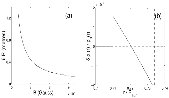
Figure 1: (a) The radius change $\delta R=R-R_{\odot}$ for various values of the magnetic field at the bottom of the convection zone. Counter-intuitively, $\delta R$ decreases with an increase in B. (b) The fractional change in density $\delta\rho(r)/{\rho_{o}(r)}$ inside the magnetic flux shell with $B=10^{5}$ G (where $\rho_{o}(r)$ is the density in the absence of magnetic fields as given by (7)). Note that for a region above $r_{b}$, the density is actually more than that below the shell!

We next try to construct a solution by assuming the plasma beta $\beta=8\pi p_{2}/B^{2}$ to be constant inside the magnetic shell. The hydrostatic equation (9) inside the magnetic shell now takes the form

$$\frac{\partial{p_{2}}}{\partial{r}}=-\frac{GM_{\odot}\rho_{2}}{(1+\beta^{-1})r^{2}}$$ (17)

Consequently $\rho_{2}(r)$ has the expression

$$\rho_{2}(r)=\Big{[}\frac{(\gamma-1)GM_{\odot}}{\gamma\kappa_{2}(1+\beta^{-1})}\Big{(}\frac{1}{r}-\frac{1}{R_{2}}\Big{)}\Big{]}^{\frac{1}{\gamma-1}}$$ (18)

When we demanded that the conditions (11), (12) and (13) are satisfied, we were able to find only one solution of the problem, which corresponds to $\beta^{-1}=0$ (i.e. no magnetic field) for which there is no change in radius. This is certainly a consistent solution, but not the solution we have been looking for.

Although we have not succeeded in constructing a satisfactory hydrostatic model, we decided to present this brief discussion as a warning to future researchers that the simplest and most obvious things do not work here. There is no doubt that (9), (11), (12) and (13) should hold. Perhaps (10) should be replaced by a more realistic thermodynamic equation and we should use the physics of magnetic field creation in more detail to decide how $B(r)$ may vary within the magnetic layer. For these more complicated cases, we shall not be able to write down an analytical solution of density as we do in (15) or (18), and consequently the solution of the problem will be much more complicated. We felt that it will be pre-mature to attempt such a solution now. Given the uncertainties in the observational data, the order-of-magnitude estimate should more than serve our purpose at present.

5 Conclusion

Within the currently understood framework of solar MHD, we have not been able to provide a theoretical explanation of the controversial claim made by Dziembowski et al. (2001) that the Sun shrinks with increasing magnetic activity at the rate of 1.5 km yr^-1. Spruit (1982, 1994) estimated the radius change due to heat blocking by sunspots near the solar surface. Not only the radius variation was found to be much smaller, the radius is expected to increase with the solar maximum. We considered the possibility if the excess magnetic pressure of flux tubes near the base of the SCZ can give us a different result. Even though traditional dynamo models regard the solar maximum as the time when the magnetic flux in the solar interior peaks and would suggest a radius increase at the time of the solar maximum, we pointed out the model of Nandy and Choudhuri (2002) provides a different scenario. Although this model would predict a decrease of the solar radius with increasing magnetic activity (i.e. with increasing loss of magnetic flux from the storage region), various reasonable assumptions give a radius decrease rate about one order of magnitude smaller than what is claimed by Dziembowski et al. (2001). It is true that our estimate is based on a very rough calculation. However, we believe that it is still an over-estimate rather than an under-estimate. Only if the magnetic field at the base of the SCZ was concentrated to values as high as $10^{6}$ G, the radius shrinkage would have been as large as reported by Dziembowski et al. (2001). There is no theoretical reason to expect a magnetic field as strong as $10^{6}$ G at the base of the SCZ. In fact, it is not easy to generate even a $10^{5}$ G magnetic field there (Choudhuri, 2003). We conclude that either the claim of Dziembowski et al. (2001) is incorrect, or else we do not understand some basic physics of the solar cycle.

References

- [1] Antia, H.M.: 2003, Astrophys. J. 590, 567.
- [2] Caligari, P. Moreno-Insertis, F., and Schussler, M.: 1995, Astrophys.J. 441, 886.
- [3] Choudhuri, A.R.:1989, Solar Phys. 123, 217.
- [4] Choudhuri, A.R.:1998, The Physics of Fluid and Plasmas: an Introduction for Astrophysicists., Cambridge University Press.
- [5] Choudhuri, A.R.: 2003, Solar Phys. , 215, 31.
- [6] Choudhuri, A.R., and Gilman, P.A. : 1987, Astrophys. J. 316, 788.
- [7] Choudhuri, A.R., Schüssler, M., Dikpati, M. : 1995, Astron. Astrophys. 303, L29.
- [8] D’Silva, S. and Choudhuri, A.R.: 1993, Astron. Astrophys. 272, 621.
- [9] D’Silva, S. and Howard, R.F.: 1993, Solar Phys. 148, 1
- [10] Dziembowski, W.A., Goode, P.R., Schou, J.: 2001, Astrophys. J. 5̱53, 897.
- [11] Emilio, M., Kuhn, J.R., Bush, R.I., and Scherrer, P.: 2000, Astrophys. J. 543, 1007.
- [12] Fan, Y., Fisher, G.H., and DeLuca, E.E.: 1993, Astrophys. J. 405, 390.
- [13] Hathaway, D. H., Nandi, D., and Wilson, R. M., Reichmann, E.J.: 2003 , Astrophys. J. 589, 665.
- [14] Moreno-Insertis, F.:1983, Astron. Astrophys. 122, 241
- [15] Nandy, D. and Choudhuri, A.R.: 2002, Science. 296, 1671.
- [16] Nöel, F.: 1997, Astron. Astrophys. 325, 825.
- [17] Parker, E.N. :1979, Cosmic Magnetic Fields: Their origin and their activity, Oxford, Clarendon Press.
- [18] Schwarzschild, M. :1958, Structure and Evolution of Stars. Dover Publications, Inc.
- [19] Spruit, H.C.: 1982, Astron. Astrophys. 108, 348
- [20] Spruit H.C. :1994, in The Solar Engine and Its Influence on Terrestrial Atmosphere and Climate, NATO ASI Series I, vol. 25 (Dordrecht:Kluwer), 107.