X-ray Preionisation Powered by Accretion on the First Black Holes. I: a Model for the WMAP Polarisation Measurement

Abstract

In this paper we investigate the possibility that there is a first phase of partial ionisation due to X-rays produced by black hole accretion in small-mass galaxies at redshifts $7<z<20$. This is followed by complete reionisation by stellar sources at $z\simeq 7$. This scenario is motivated by the large optical depth to Thompson scattering, $\tau_{\rm e}$ $\simeq 0.17\pm 0.04$, recently measured by WMAP. But it is also consistent with the observed Gunn-Peterson trough in the spectra of quasars at $z\sim 5-6$. We use a semianalytic code to explore models with different black hole accretion histories and cosmological parameters. We find that “preionisation” by X-rays can increase the intergalactic medium (IGM) optical depth from $\tau_{\rm e}$ $\approx 0.06$ given by stellar sources only, to $0.1\lower 2.15277pt\hbox{$\;\buildrel<\over{\sim}\;$}\tau_{\rm e}\lower 2.15277pt\hbox{$\;\buildrel<\over{\sim}\;$}0.2$, if a fraction of baryons $10^{-5}\lower 2.15277pt\hbox{$\;\buildrel<\over{\sim}\;$}\omega_{\rm ac}\lower 2.15277pt\hbox{$\;\buildrel<\over{\sim}\;$}10^{-4}$ is accreted onto seed black holes produced in the collapse of low metallicity, high mass stars before $z\simeq 15$. To be effective, preionisation requires a non-negligible star formation in the first small-mass galaxies in which seed black holes are formed. By $z\sim 20-25$ the IGM is re-heated to $10,000$ K and the ionisation fraction is about 20%. The increase of the IGM Jeans mass is effective in reducing star formation in the smaller-mass haloes. Large values of $\tau_{\rm e}$ are obtained in models with top-heavy stellar initial mass function only if pair-instability supernovae are not important. Seed black holes are assumed to accrete at near the Eddington limit with a duty cycle that decreases slowly with increasing time. Alternatively, a moderate fraction of the black holes must be ejected from the host galaxy or exist without merging into the supermassive black holes in galactic centres. The model predicts that dwarf spheroidal galaxies, if they are preserved fossils of the first galaxies, may host a mass in black holes that is 5-40% of their stellar mass. The redshifted X-ray background produced by this early epoch of black hole accretion constitutes about $5-10$% of the X-ray background in the 2-50 keV bands and roughtly half of the currently estimated black hole mass density was formed at early times. Moreover, in most models, the photons from the redshifted background are sufficient to fully reionise He ii at redshift $z\sim 3$ without any additional contribution from quasars at lower redshifts and the temperature of the mean density intergalactic medium remains close to $10^{4}$ K down to redshift $z\sim 1$.

1 Introduction

The mean transmitted flux along the line of sight of the furthest quasars found by the Sloan Digital Sky Survey (e.g., Becker et al., 2001) shows that the ionisation fraction of the intergalactic medium (IGM) is rapidly decreasing approaching $z\sim 6.3$. Assuming, at that redshift, an approximately constant stellar emissivity of ionising radiation, the IGM would have been reionised at $z_{\rm rei}$ $\sim 7$ by stellar sources (Gnedin, 2000a; Djorgovski et al., 2001; Songaila & Cowie, 2002; Fan et al., 2003, and others). But a much earlier ionisation epoch is implied by the WMAP observations (Bennett et al., 2003; Kogut et al., 2003). If the IGM had a sudden transition from neutral to completely ionised, producing the optical depth to Thompson scattering $\tau_{\rm e}$ $=0.17\pm 0.04$ measured by WMAP, $z_{\rm rei}$ $\simeq 17$ for the best fit $\Lambda$CDM cosmological model (Spergel et al., 2003).

In a companion paper (paper I, Ricotti & Ostriker, 2004), we have tried to explain these apparently contradictory results by considering the contribution to reionisation due to zero-metallicity (Population III) stars. Since such stars are thought to be massive ($M_{*}>5-10$ M_⊙) (e.g., Omukai & Nishi, 1998; Abel et al., 2000; Bromm et al., 2002; Abel et al., 2002; Nakamura & Umemura, 2002) and hot (Tumlinson & Shull, 2000), their efficiency for UV emission is larger than for Population II and Population I stars that have a Salpeter initial mass function (IMF). A time dependent efficiency of UV emission, $\epsilon_{\rm UV}$, produced by the transition from a top-heavy IMF at high redshift to a Salpeter IMF at low redshift, could possibly explain the large $\tau_{\rm e}$ measured by WMAP and would be consistent with the Sloan data at $z\lower 2.15277pt\hbox{$\;\buildrel<\over{\sim}\;$}6.3$ (Chiu et al., 2003). An upper limit of the UV emissivity, $\epsilon_{\rm UV}^{\rm max}\lower 2.15277pt\hbox{$\;\buildrel<\over{\sim}\;$}2-3\times 10^{-3}$ can be derived by assuming the maximum efficiency of energy production by thermonuclear reactions in massive stars. For a Salpeter IMF, $\epsilon_{\rm UV}\sim 2-4\times 10^{-4}$, depending on the stellar metallicity (Tumlinson & Shull, 2000). Therefore, assuming a constant (maximal) escape fraction of ionising photons from the galaxies, $\langle f_{\rm esc}\rangle$ $\simeq 1$, a redshift dependent IMF would increase the UV emission efficiency from low to high redshift by about 10-20 times.

Several authors have tried to reproduce the high optical depth measured by WMAP with the increased ionising photon emission by zero-metallicity stars. Cen (2003) has used a semianalytic calculation to indicate that the IGM may have experienced two distinct epochs of reionisation. Haiman & Holder (2003) have investigated different reionisation histories showing that optical depths consistent with WMAP can be achieved assuming very massive Population III stars. Wyithe & Loeb (2003) show that, if feedback regulates star formation in early low-mass galaxies as observed in present-day dwarfs, Population III stars forming with a heavy IMF are required to match WMAP data. Ciardi et al. (2003), using numerical simulation, show that zero metallicity stars with a moderately heavy IMF (characteristic stellar mass of 5 M_⊙) and $\langle f_{\rm esc}\rangle$ $=20$% are able to generate an optical depth of 0.17, consistent with WMAP data. Sokasian et al. (2004), also using numerical simulations, showed that zero metallicity stars with a top-heavy IMF and $\langle f_{\rm esc}\rangle$ $\sim 100$% is needed to produce an optical depth consistent with WMAP data.

In paper I we have found (consistent with the work of the other investigators mentioned above) that, assuming the most extreme properties for zero metallicity stars (top heavy IMF and $\langle f_{\rm esc}\rangle$ $\sim 100$%), the maximum optical depth to Thomson scattering produced by Population III stars is $\tau_{\rm e}$ $\sim 0.13$, marginally consistent with WMAP data. In order to produce this large value of $\tau_{\rm e}$, massive zero-metallicity (Population III) stars must be the dominant population until redshift $z\simeq 10$. But we have noted that, if the ratio of metal atoms to ionising photons produced by Population III stars is normal, the metal enrichment of the ISM prevents metal-poor stars from being produced for long enough to ionise more than a small fraction of the IGM, i.e.that the Population III phase is very rapidly self-limiting. In addition, if pair-instability SNe are important, the mechanical energy input by SN explosions produces strong outflows in galaxies with masses $M_{\rm dm}\lower 2.15277pt\hbox{$\;\buildrel<\over{\sim}\;$}10^{9}$ M_⊙, reducing their star formation and delaying reionisation. These two effects will lower the redshift of reionisation and $\tau_{\rm e}$ to values inconsistent with WMAP but still consistent with the Sloan quasar data. Thus we have found it essentially impossible to reproduce the WMAP and Sloan results using stellar sources of UV ionisation.

In summary, the reason for the partial disagreement with the conclusions of previous works on the ability of Population III stars to produce the large optical depth observed by WMAP, is motivated by our findings concerning the self-termination of Population III stars by the enhanced metal pollution and the negative feedback on star formation from the enhanced energy input by SN explosions, that inevitably follow from the assumption of a top-heavy IMF. In previous works these concerns have not been addressed. However in paper I we also note that, if most Population III stars collapse into black holes (BHs), the metal pollution problem is alleviated and the mechanical feedback from SN/hypernova explosions will be reduced as well. An interesting consequence of this scenario is a copious production of BHs from the first stars (Schneider et al., 2002). For this reason it is possible that the secondary radiation from accretion onto seed BHs might be a more important source of ionising radiation than the primary radiation from the same stars. In particular because, as we will show, accretion on seed BHs is not sensitive to the early termination of the Population III epoch by metal pollution.

Motivated by these results, in this paper we study the partial ionisation of the IGM by an early X-ray background produced by accreting BHs, followed by more complete stellar reionisation by Population II stars at $z_{\rm rei}$ $\approx 7$. An hybrid model where UV from Population III stars and X-ray emission from accreting BHs are both important in producing a large optical depth is also viable if self-termination of Population III stars happens late (e.g., $z\sim 10$) and if we assume extreme parameters for $\langle f_{\rm esc}\rangle$ and for the global Population III stars UV emissivity. But, given the difficulties in modelling properly the transition from Population III to Population II stars, the predicted importance of UV from Population III stars is very uncertain (almost a free parameter at this point). As an example, in the present paper we show a model where the transition from Population III to Population II stars is at redshift $z\sim 15$. In this case we show that UV radiation from Population III stars has negligible effect on the Thompson optical depth.

For a fixed emissivity of ionising radiation, X-rays are less efficient in reionising the IGM, because most of their energy goes into heat instead of ionisation. The inclusion of secondary electrons can boost the ionisation efficiency by about a factor of ten if the electron fraction of the IGM is $\langle x_{\rm e}\rangle$ $<10$ %, but roughly $1/3$ of the primary electron energy is always converted into heating of the IGM (Shull & van Steenberg, 1985). It will be shown that the partial ionisation of the IGM must begin at redshifts $z\lower 2.15277pt\hbox{$\;\buildrel>\over{\sim}\;$}15$ in order to have an important effect on $\tau_{\rm e}$. This can only happen if the X-ray sources (i.e., accreting BHs) form in small-mass haloes with masses $M_{\rm dm}\lower 2.15277pt\hbox{$\;\buildrel<\over{\sim}\;$}10^{8}$ M_⊙. Previous work on the formation of the first galaxies (Ricotti et al., 2002a, b) has used cosmological simulations with radiative transfer to show that star formation in the first small-mass galaxies is reduced by feedback effects but is not suppressed. It is therefore plausible that a substantial production of seed BHs from the first stars took place in the first small-mass galaxies.

Published studies have investigated the effects of X-rays on early galaxy formation using a semianalytic approach (Oh, 2001; Venkatesan et al., 2001) and cosmological simulations (Machacek et al., 2003). But since those works were completed before WMAP results, they did not focus on scenarios that could produce $\tau_{\rm e}$ $\simeq 0.17$. The study presented in this paper (paper IIa) is carried out using a semianalytic code based on principles similar to those adopted by Chiu & Ostriker (2000). In Ricotti, Ostriker, & Gnedin (2004) (paper IIb) we present the results of cosmological hydrodynamic simulations that include radiative transfer. We discuss the observational signatures of X-ray preionisation compared to stellar reionisation, including calculations of the expected amplitude of secondary anisotropies of the CMB and the redshifted 21cm signal in absorption and emission against the CMB. The semianalytic models presented in this paper allow us to explore a larger parameter space and help us to interpret the numerical result of the full cosmological simulations. This new code, presented in Appendix A, calculates the evolution of the filling factor of H ii regions and the ionisation and thermal history of the IGM outside the H ii regions, produced by an X-ray background. The semianalytic code has been tested and calibrated using the results of the cosmological simulations (cf., paper I). Note that some cosmological simulations presented here include the effects of SN explosions, using the recipe discussed in Gnedin (1998), in contrast to earlier papers in this series (Ricotti et al., 2002a, b).

This paper is organised as follows. In § 2 we present qualitative arguments showing why and for which models X-ray preionisation can be more effective in increasing $\tau_{\rm e}$ than reionisation by stellar sources. In § 3 we estimate the accretion rate onto seed BHs and we compute the integrated X-ray energy required to explain the large $\tau_{\rm e}$ measured by WMAP. In § 4 we summarise the characteristics of the semianalytic code for reionisation and we show its results. In § 5 we conclude this work with a summary and a discussion of some of the observable effects of early black hole X-ray heating. A full description of the semianalytic code is given in Appendix A.

2 X-Ray preionisation: rationale

The essential physics is easily understood. Ultraviolet (UV) photons from stars at wavelengths only moderately shorter than $912$ Å  ($h\nu=13.6$ eV) have a very short mean free path in neutral hydrogen. As a consequence they produce Strömgren spheres surrounding the UV sources in high density regions. In such regions recombination rates are high and many photons are required to keep one hydrogen atom ionised for a Hubble time. The much larger volumes between the Strömgren spheres remain sensibly neutral. However, much harder photons (e.g., 1 keV) can uniformly fill space and thus lead to fractional ionisation which is higher in the low-density regions than in the high-density regions containing the sources. But, as noted earlier, the fractional ionisation is low but the volume is large since the volume fraction in virialised haloes at $z=15$ is only a few per cent. To illustrate this let us show how a simple ad hoc ionisation history affects $\tau_{\rm e}$. In Fig. 1, we show the IGM optical depth to Thompson scattering, $\tau_{\rm e}$, in a model where a complete reionisation at redshift $z_{\rm rei}$ is preceded by a partial ionisation, with constant ionisation fraction $\langle x_{\rm e}\rangle$, starting at $z=z_{\rm PBH}$. The long-dashed, dashed, dotted and solid lines in Fig. 1 show $\tau_{\rm e}$ as a function of $z_{\rm PBH}$ assuming complete reionisation at $z_{\rm rei}$ $=7$ and preionisation electron fraction $\langle x_{\rm e}\rangle$ $=0.7,0.5,0.3$ and 0.2, respectively. We see that two conditions need to be met in order to have $\tau_{\rm e}$ $\simeq 0.17$: (i) preionisation must start early, at $z_{\rm PBH}\sim 20-40$, and (ii) the IGM preionisation fraction must be $\langle x_{\rm e}\rangle$ $\lower 2.15277pt\hbox{$\;\buildrel>\over{\sim}\;$}20$%.

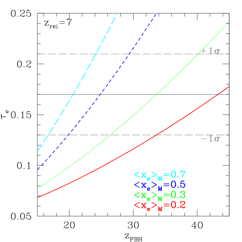
Figure 1: Optical depth to Thomson scattering, $\tau_{\rm e}$, for a toy model where a complete reionisation at redshift $z_{\rm rei}$ $=7$ is preceded by constant, partial ionisation $\langle x_{\rm e}\rangle$, starting at redshift $z=z_{\rm PBH}$. The lines from bottom to the top refer to mean (mass weighted) ionisation fractions $\langle x_{\rm e}\rangle$ ${}_{M}=0.2,0.3,0.5$, and $0.7$.

Condition (i) is met only if the X-ray sources can form in haloes with masses $M_{\rm dm}\lower 2.15277pt\hbox{$\;\buildrel<\over{\sim}\;$}10^{8}$ M_⊙. The two peculiarities of these small-mass haloes are that they rely on molecular hydrogen cooling to form stars, and their dark matter gravitational potential is too shallow to retain gas hotter than $T\approx 2\times 10^{4}$ K. For these reasons small-mass galaxies are subject to radiative feedback effects that might suppress their formation (e.g., Haiman et al., 1997; Machacek et al., 2003, but see Ricotti et al., 2001, who find a new positive feedback effect). Using cosmological simulations with radiative transfer Ricotti et al. (2002a, b) found that the main negative feedback thought to suppress the formation of the first galaxies (the H₂ photodissociating background) is not the dominant effect. Instead, feedback by ionising radiation plays the dominant rôle, inducing a bursting star formation mode in small-mass galaxies. The feedback mechanism is complex because it is composed of several processes, each with different relevance depending on the parameters of the simulation (mainly the ionising escape fraction, $\langle f_{\rm esc}\rangle$, and the IMF). In brief, photoevaporation and H₂ formation/photodissociation produce a bursting mode of star formation that is catalyst for molecular hydrogen re-formation inside relic H ii regions and in the precursors of cosmological Strömgren spheres. Star formation in small-mass galaxies is self-regulated on a cosmological scale and it is reduced by radiative feedback but is not suppressed. Even if the volume fraction filled with ionised Strömgren spheres never exceeds a few per cent, these small-mass galaxies form enough Population III stars and therefore seed black holes (see § 3) to produce, via accretion, a substantial X-ray background at high redshift.

Condition (ii) can be met if the X-ray energy input is sufficiently large. Note that ionisation by secondary electrons becomes increasingly inefficient when $\langle x_{\rm e}\rangle$ $\lower 2.15277pt\hbox{$\;\buildrel>\over{\sim}\;$}10-20$% since the secondary electrons loose an increasing fraction of their energy to heat and a decreasing fraction to further ionisation as the neutral fraction declines. We can estimate the fraction of baryons, $\omega_{\rm ac}$, that we need to accrete by counting the number of ionisations per hydrogen atom, $N_{\rm Xph}\simeq$$\langle x_{\rm e}\rangle$, needed to partially ionise the IGM to a level $\langle x_{\rm e}\rangle$ $\sim 50$% (the fractional ionisation of the IGM must be $\langle x_{\rm e}\rangle$ $\lower 2.15277pt\hbox{$\;\buildrel>\over{\sim}\;$}20$% in order to produce the large optical depth to Thomson scattering measured by WMAP, cf. Fig. 1). If we neglect recombinations we have

$$N_{\rm Xph}=7.3\times 10^{7}\left(\epsilon_{\rm X}\over X_{\rm Xsec}\right)\omega_{\rm ac}\simeq\langle x_{\rm e}\rangle\simeq 0.5,$$ (1)

where $\epsilon_{\rm X}$ is the energy emitted in the X-ray band per hydrogen atom accreted on the BHs and $X_{\rm Xsec}$ is a pure number defined as $X_{\rm Xsec}=X_{\rm X}/f_{\rm sec}\sim 20$, where $f_{\rm sec}\sim 5-10$ takes into account the extra ionisation by secondary electrons (we have estimated this number switching off secondary ionisations in our semianalytic code, presented in the appendix), and $X_{\rm X}=\overline{h\nu}/(13.6{\rm eV})$ is the mean energy of X-ray photons in units of the H i ionisation energy for the assumed X-ray spectrum. For accretion around a BH in which the gas is highly ionised and electron scattering is the most important opacity, the isotropic luminosity produced by the accretion cannot exceed the Eddington luminosity

$$L_{\rm Ed}\equiv{4\pi GM_{\rm BH}m_{p}\over\sigma_{T}}=(1.3\times 10^{38}{\rm erg~{}s}^{-1})\left({M_{\rm BH}\over M_{\odot}}\right),$$ (2)

where $\sigma_{T}$ is the Thomson scattering cross section. Given the accretion efficiency $\epsilon=L/\dot{M}_{\rm ac}c^{2}\sim 0.15$, typical for quasars, the mass accreted at the Eddington rate is $\dot{M}_{\rm Ed}=L_{\rm Ed}/\epsilon c^{2}$ and the timescale of the accretion is the Eddington time $t_{\rm Ed}=M_{\rm BH}/\dot{M}_{\rm Ed}\sim 10^{8}$ yrs.

Observations of active galactic nuclei (AGN) at low-redshift show that, when the central BH is accreting, it does so at near the Eddington limit and, when it is quiet, the energy output is negligible. In § 3 we will introduce a parameter, $f_{\rm duty}$, to model the observed duty cycle of AGN. We define $f_{\rm duty}$ as the fraction of time when the BH is accreting at the Eddington limit. Assuming a spectral energy distribution (SED) typical for AGNs (cf., Fig. 4), a fraction $\beta=L_{\rm X}/L_{\rm Ed}\sim 10$% of the energy output from the accreting BH is emitted in the X-ray band, with a resulting efficiency of X-ray production $\epsilon_{\rm X}=\beta\epsilon$. Finally, using equation (1), we can estimate the fraction of baryons that needs to be accreted to partially reionise the IGM,

$$\omega_{\rm ac}\simeq 6.8\times 10^{-6}\left({0.02\over\epsilon_{\rm X}}\right)\left({X_{\rm Xsec}\over 20}\right).$$ (3)

As a comparison we also estimate the baryon fraction needed to be converted into stars to reionise the IGM. The maximum radiative efficiency from thermonuclear processes is $\epsilon_{\rm UV}^{\rm max}=2-3\times 10^{-3}$. Since UV photons have a short mean free path they first ionise, and keep ionised, the high density regions around each source before escaping into the IGM. In this case, then we cannot neglect recombinations. The number of UV photons per baryon needed to reionise the IGM is $N_{\rm UVph}\simeq C_{{\text{H\,\sc ii}}}\simeq 10$, where $C_{{\text{H\,\sc ii}}}=\langle n_{\rm e}^{2}\rangle/\langle n_{\rm e}\rangle^{2}$ is the effective clumping factor of the ionised gas. Note that the effective clumping, $C_{{\text{H\,\sc ii}}}$, is the time averaged clumping of the IGM from the time the first source turns on to the time of reionisation. When the volume filling factor of the Strömgren spheres is small the clumping factor of the ionised gas is very large, but equals the clumping of the gas, $C$, at the redshift of reionisation (see Fig. 4 in paper I). In addition, the escape fraction of ionised photons, $\langle f_{\rm esc}\rangle$, and the value of $C_{{\text{H\,\sc ii}}}$ are related to each other and depend on the resolution of the hydrodynamic simulation or on the definition of $\langle f_{\rm esc}\rangle$ in semianalytic models. Keeping in mind these caveats, the fraction of baryons that needs to be converted into Population III stars to reionise the IGM is approximately

$$\omega_{*}\simeq 4\times 10^{-4}\left({C_{{\text{H\,\sc ii}}}\over 10}\right)\left({0.5\over\langle f_{\rm esc}\rangle}\right)\left({2\times 10^{-3}\over\epsilon_{\rm UV}}\right)\left({X_{\rm UV}\over 3}\right),$$ (4)

where $X_{\rm UV}=\overline{h\nu}/(13.6{\rm eV})$ is the mean energy of UV photons in units of the H i ionisation energy for a Population III spectrum. By comparing equation 4 to equation 3 it is evident that the baryon fraction that needs to be accreted onto BHs to partially reionise the IGM to $\langle x_{\rm e}\rangle$ $=0.5$ is about 60 times smaller than the fraction of baryons that needs to be converted into massive Population III stars. This shows that X-rays from accreting BHs are potentially more efficient than UV from stars in producing a large $\tau_{\rm e}$.

Observations in the soft X-ray bands of Lyman-break galaxies (which do not contain AGNs) at redshift $z\sim 3$ (Nandra et al., 2002) have shown that their soft X-ray emission is proportional to the UV emission: $L_{\rm X}/L_{\rm UV}\sim 0.01$. This emission, attributed to X-ray binaries and SN remnants, is too low to influence preionisation. In addition, about 3% of Lyman-break galaxies contain central AGNs, accreting at roughly the Eddington limit (Steidel et al., 2002). X-ray emission powered by accretion on primordial seed BHs could thus be important. There are two scenarios for the formation of supermassive black holes (SMBHs) in the bulges of today’s galaxies: monolithic collapse, or mergers and accretion on seed BHs. Only the mass growth due to accretion produces X-rays available to ionise the IGM. Assuming that most of the mass in SMBHs observed in the bulges of galaxies at $z=0$ has been accreted at high redshift, the upper limit for the accreted mass is

$$\omega_{\rm BH,max}=\left({M_{\rm SMBH}\over M_{\rm bulge}}\right)\omega_{\rm bulge}=(1\pm 0.7)\times 10^{-4},$$ (5)

where we used $M_{\rm SMBH}/M_{\rm bulge}=(1.5\pm 0.3)\times 10^{-3}$ (e.g., Kormendy & Richstone, 1995; Gebhardt et al., 2000) and $\omega_{\rm bulge}=(6.5\pm 3)\%$ (Persic & Salucci, 1992; Fukugita et al., 1998). But another scenario is possible in which BH seeds grow through accretion at high redshift to a level higher than currently observed, but a significant fraction of them is expelled from the galaxies or does not end up in the observed population of SMBHs. In this case a fraction of the halo DM would be made of primordial BHs. The recent discovery of several ultra-luminous X-ray sources (ULX) has been interpreted as evidence for intermediate-mass BHs (about 100 M_⊙). These objects could also be relics of primordial BHs.

In summary, X-rays may be more effective in increasing the optical depth to electron Thompson scattering $\tau_{\rm e}$ with respect to UV photons from stellar sources for the following reasons:

• X-rays escape unabsorbed from the ISM of galaxies while for UV radiation $\langle f_{\rm esc}\rangle$ $<1$.

• X-rays ionise preferentially the low-density regions where the clumping factor is $C_{{\text{H\,\sc ii}}}<1$. Consequently, the recombination rate is reduced.

• X-rays only partially ionise the IGM: $\langle x_{\rm e}\rangle$ $\sim 20-70$%. This reduces the recombination rate by a factor $\langle x_{\rm e}\rangle$.

• The emission efficiency of radiation due to gravitational accretion can be as high as $\epsilon\simeq 0.15$ (accretion at the Eddington limit). This efficiency is about 100 times the maximum efficiency produced by thermonuclear reactions in stars $\epsilon_{\rm UV}^{\rm max}\simeq 2\times 10^{-3}$.

• The accretion on seed BHs can continue even if the epoch of Population III star domination is very short due to the metal pollution of the star forming gas.

On the other hand, X-rays may be inefficient with respect to UV radiation in ionising the IGM for the following reasons:

• X-rays have to be emitted at early times to be effective. This can only happen if a substantial density of seed BHs is formed in small-mass galaxies, at $z\lower 2.15277pt\hbox{$\;\buildrel>\over{\sim}\;$}20$.

• X-rays are less efficient in ionising than UV photons. But, if the electron fraction in the IGM is $\langle x_{\rm e}\rangle$ $\lower 2.15277pt\hbox{$\;\buildrel<\over{\sim}\;$}10-20$ %, secondary electrons are an important additional source of ionisation. Nevertheless, as we will show in § 4.2, hard-UV photons and the redshifted X-ray background can enhance the IGM electron fraction to levels well above $\langle x_{\rm e}\rangle$ $\sim 10-20$%.

• X-rays are efficient in heating the IGM and therefore they increase the IGM Jeans mass. This will have a negative feedback on the formation of the smaller mass galaxies and consequently on the formation of seed BHs and their ability to accrete gas.

3 Mass Accretion History on seed BHs

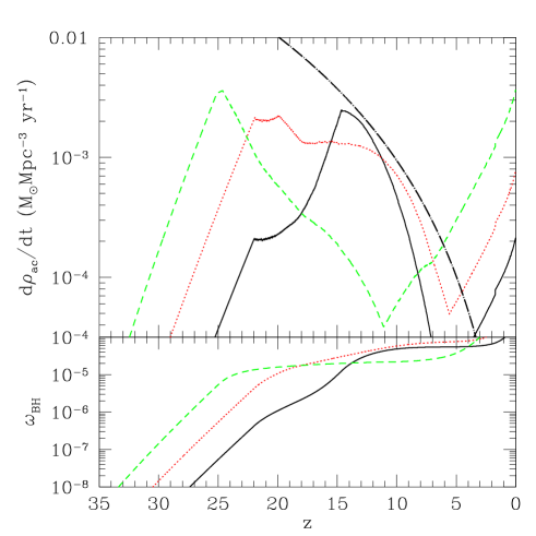
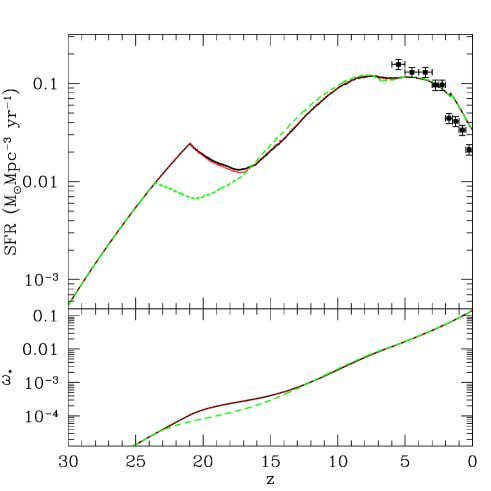
Figure 2: (left) The top panel shows the black hole accretion rate, $\dot{\rho}_{\rm ac}\equiv\rho_{0}\dot{\omega}_{\rm ac}$ (where $\rho_{0}$ is the cosmic baryon density at $z=0$ and $\omega_{\rm ac}$ is given in equation [7]), as a function of redshift. The bottom panel shows the baryon fraction in BHs, $\omega_{\rm BH}$, as a function of redshift. (right) The top panel shows the star formation rate, $\dot{\rho}_{*}\equiv\rho_{0}\dot{\omega}_{*}$, as a function of redshift. The bottom panel shows the baryon fraction in stars as a function of redshift. The solid, dotted and dashed lines refer models M3, M4, and M5 in table 2, respectively. The dot-dashed line in the top panel of the left figure is an upper limit for the accretion rate given by equation (11).

The formation rate of seed black holes from star formation is very uncertain. The calculations of the mass of the remnant and metal yields are strongly dependent on the energy of the SN explosion, $E_{51}=E/10^{51}$ erg, on the mass shell at which the explosion takes place and the star metallicity. These numbers are uncertain and calculations (Woosley & Weaver, 1995) have been done for a grid of models. In table 1 we list the fraction, $f_{\rm BH}$, of stellar mass expected to end in seed BHs for the different explosion models, gas metallicities and stellar IMF. The data is from Woosley & Weaver (1995): Model A has $E_{51}\sim 1$; Model B has $E_{51}\sim 2$; and Model C has $E_{51}\sim 3$. The values listed in the table are the weighted means of $f_{\rm BH}$ for stellar masses between $12~{}{\rm M}_{\odot}<M_{*}<40$ M_⊙ with weight $M^{\alpha}$. Note that for a Salpeter IMF ($\alpha=-1.35$) with stellar masses between $1~{}{\rm M}_{\odot}<M_{*}<100$ M_⊙, the mass in stars with $M_{*}>8$ M_⊙ is 20 % of the total.

Very massive stars (VMS) in the mass range $140~{}{\rm M}_{\odot}<M_{*}<260$ M_⊙ are believed to explode completely without leaving any remnant due to an instability produced by annihilation of electrons and positrons (pair-instability SNe) and hence have $f_{\rm BH}=0$. Stars more massive than $M_{*}=260$ M_⊙ are believed to collapse directly into BHs, without exploding as SNe and hence have $f_{\rm BH}=100$% (Heger & Woosley, 2002). The existence of a mixture of masses for supermassive Population III stars allows for all possible values of $f_{\rm BH}$ from zero to unity.

Table 1: Fraction of stellar mass that forms seed BHs

$Z/Z_{\odot}$		$f_{\rm BH}$ (%)		IMF
	Model A	Model B	Model C	$\alpha$
$0$	19	12	11	-1.35
$0$	24	12	8	0
$0$	24	13	7	1
$10^{-4}$	10	8	8	-1.35
$10^{-4}$	13	8	7	0
$10^{-4}$	16	8	7	1
$1$	11	10	8	-1.35
$1$	13	10	8	0
$1$	15	10	8	1

The mass growth of seed BHs can be calculated if we know the accretion rate $\dot{\omega}_{\rm ac}$ of BHs, the formation rate of seed BHs, $\dot{\omega}_{\rm seed}$, and the ejection rate of BHs from galaxy haloes, $\dot{\omega}_{\rm ej}$. To calculate the mass growth of BHs we solve the following equation:

$$\dot{\omega}_{\rm BH}=\dot{\omega}_{\rm ac}-\dot{\omega}_{\rm ej}+\dot{\omega}_{\rm seed},$$ (6)

where $\omega_{\rm BH},\omega_{\rm ac},\omega_{\rm ej}$ and $\omega_{\rm seed}$ are expressed as a fraction of the baryon content of the universe. The accretion rate is proportional to $\omega_{\rm BH}$, independently of the mass function of BHs,

$$\dot{\omega}_{\rm ac}=f_{\rm duty}{\omega_{\rm BH}\over t_{\rm Ed}},$$ (7)

where the accretion time, $t_{\rm ac}\equiv t_{\rm Ed}/f_{\rm duty}$, is expressed as the fraction of time, $f_{\rm duty}$, that the BHs are accreting at the Eddington rate. If we assume that the BH accretes at the Eddington limit for a time interval $t_{on}$ and stops accreting for a time interval $t_{\rm off}$, the duty cycle parameter is $f_{\rm duty}=t_{\rm on}/(t_{\rm off}+t_{\rm on})<1$. If we neglect BH ejection we have

$$\dot{\omega}_{\rm BH}=f_{\rm duty}{\omega_{\rm BH}\over t_{\rm Ed}}+f_{\rm BH}\dot{\omega}_{*},$$ (8)

where we have assumed that the formation rate of seed BHs is a fraction, $f_{\rm BH}$, of the star formation rate $\dot{\omega}_{\rm seed}=f_{\rm BH}\dot{\omega}_{*}$ (see table 2). Integrating equation (8) we get

$$\omega_{\rm BH}(t)=\int_{0}^{t}dt^{\prime}f_{\rm BH}\dot{\omega}_{*}(t^{\prime})\exp{[F(t)-F(t^{\prime})]},$$ (9)

where,

$$F(t)={1\over t_{\rm Ed}}\int_{0}^{t}f_{\rm duty}dt^{\prime}.$$

We parameterise the duty cycle as

$$f_{\rm duty}(z)=\left({1+z\over z_{\rm BH}}\right)^{\phi},$$ (10)

and imposing the condition $0.001\leq f_{\rm duty}\leq 1$ to be consistent with the observed fraction of AGN $f_{\rm duty}\lower 2.15277pt\hbox{$\;\buildrel<\over{\sim}\;$}3$% at $z\sim 3$ (Steidel et al., 2002), and $f_{\rm duty}\sim 0.001$ at $z=0$.

In this work we will not attempt to investigate in detail the physical processes and feedback effects that could produce the duty cycle given in equation (10). Here we simply point out the existence of, at least, one simple physical model that can reproduce the family of equations given in (10). In this model the time $t_{\rm off}$ during which the BH is quiescent is the Compton cooling time $t_{\rm Comp}=(224~{}{\rm Myr})[(z+1)/10]^{-4}$. This is the time that it takes for the gas in the proximity of the BH to cool and be accreted after the temporary halt of the accretion produced by gas heating from the previous BH activity. If we further assume that the duration of the burst is a fraction, $\eta$, of the Eddington time ($t_{\rm on}=\eta t_{\rm Ed}$) we can reproduce $f_{\rm duty}\equiv 1/(1+t_{\rm off}/t_{\rm on})$ with the form given in equation (10), where the value of $z_{\rm BH}$ is determined by the value of $\eta$. For reasonable values of $\eta$ in the range $1-100$% it is possible to describe models spanning from the early (i.e., adopting $\eta\sim 1$%) to the late preionisation (i.e., adopting $\eta\sim 100$%). On the basis of observations of AGNs at redshift $z\lower 2.15277pt\hbox{$\;\buildrel<\over{\sim}\;$}3$, the best estimate of $t_{\rm on}$ is $\sim 10$ Myr (e.g., Haehnelt et al., 1998). This suggests that the intermediate preionisation models (that adopt $\eta\sim 10$%) are prefered.

For the purpose of this paper we do not need to focus on the functional form of the duty cycle at low redshifts ($z\lower 2.15277pt\hbox{$\;\buildrel<\over{\sim}\;$}3$) provided that we can avoid to violate observational constraints on the duty cycle and BH accretion rate. In order to get a realistic accretion rate at lower redshift in some models, it might be necessary to adopt a non zero ejection rate of BHs from the host galaxies [i.e., $\dot{\omega}_{\rm ej}\not=0$ in equation (6)]. Also this assumption has physical motivations (e.g., Madau et al., 2004).

In § 4 we use a semianalytic code to follow the chemical and thermal history of the IGM in models where accretion on seed BHs partially ionise the universe. At redshift $z\approx 6.3$ stellar sources reionise the IGM to a level consistent with Sloan quasar observations. We explore three cases that differ for the accretion history onto seed BHs. The accretion history, parametrised using the equations derived in this section, can happen early ($z\sim 25$), late ($z\sim 15$) or at intermediate redshifts ($z\sim 20$). If we wished to allow for a lag, $\Delta t$, between the formation of an individual BH and the commencement of accretion on it (cf., Madau et al., 2004; Whalen et al., 2003) we would simply replace $\dot{\omega}_{*}(t^{\prime})$ with $\dot{\omega}_{*}(t^{\prime}-\Delta t)$ in equation (9). In table 2 we list the parameters adopted for the semianalytic simulations whose results will be shown in § 4. The values for $f_{\rm BH}$ allow for a range of mass functions from Salpeter to top-heavy. We also set $f_{\rm BH}=0$ in all models after $z=15$ since the formation of Population III stars that produce the seed BHs is probably self-terminated by metal enrichment well before reionisation at $z_{\rm rei}=7$. But this assumption does not have any effect on the BH accretion history because the total mass in BHs becomes dominated by the accretion on e-folding time scales $t\sim t_{\rm ac}$, making the contribution by further seed BH formation negligible after the initial phase (before the global accretion rate reaches the maximum).

Table 2: Parameter of the semianalytic models

Model	$f_{\rm BH}$ (%)	$\phi$	$z_{\rm PBH}$ ($t_{\rm on}$ Myr)	$n_{\rm s}$	$z_{\rm PopIII}$
M3	0.2	12	15  ($\sim 100$)	1.00	-
M3b	0.1	8	15  ($\sim 100$)	1.04	-
M4	2	8	20  ($\sim 10$)	1.00	-
M4b	2	8	20  ($\sim 10$)	1.00	15
M5	20	12	25  ($\sim 1$)	1.00	-

Meaning of the parameters: $f_{\rm BH}$ is the fraction of stellar mass that collapses into BHs; $\phi$ and $z_{\rm PBH}$ are the parameters in equation 10 that determines the time evolution of the duty cycle $f_{\rm duty}$; $n_{\rm s}$ is the spectral index of the spectrum of primordial density perturbations; $z_{\rm PopIII}$ is the redshift at which UV radiation from Population III stars (that has emissivity 11 times larger than the UV from Population II stars) begins to fade: the function for the UV emissivity is given by $\epsilon_{\rm UV}(z)/\epsilon_{\rm UV}(z=0)=10\{\arctan{[2(z-z_{\rm PopIII})]}/\pi+0.5\}+1$, where the emissivity from Population II stars (that is used in all the other models) is $\epsilon_{\rm UV}(z=0)=4.8\times 10^{-5}$.

The BH accretion rate as a function of redshift, $\dot{\rho}_{\rm ac}(z)\equiv\rho_{0}\dot{\omega}_{\rm ac}$, where $\rho_{0}$ is the cosmic baryon density at $z=0$ and $\omega_{\rm ac}$ is given in equation (7), is shown in the top panel of Fig. 2(left). The baryon fraction in BHs, $\omega_{\rm BH}$, as a function of redshift is shown in the bottom panel of Fig. 2(left). The solid, dotted and dashed lines refer models M3, M4, and M5 in table 2, respectively. As already noted, all the models have about the same $\omega_{\rm BH}\sim 10^{-4}$ at $z=0$ (i.e., the same total energy output from the sources) and differ for the characteristic epoch of accretion. The BH accretion rate is always negligible at the redshift, $z_{\rm rei}$, of IGM reionisation by stellar sources. The dot-dashed line shown in the top panel of the Fig. 2(left) is an upper limit for the accretion rate. This limit on the accretion rate is given by equation (11), that will be discussed in § 4.2.

In Fig. 2(right) we show the star formation rate (top panel) and the baryon fraction in stars, $\omega_{*}$ (bottom panel), as a function of redshift for the same models (cf., table 2). The points with errorbars in the top panel show the observed SFR from (Lanzetta et al., 2002). The baryon fraction in stars at redshift $z=0$ is $\omega_{*}=20$% in all the models, consistent with observations (Persic & Salucci, 1992). The feedback due to the X-ray heating of the IGM suppresses galaxy formation in haloes with masses smaller than the IGM filtering mass, producing the substantial reduction of the global SFR observed at redshifts around $z=15$ in the top panel of Fig. 2(right).

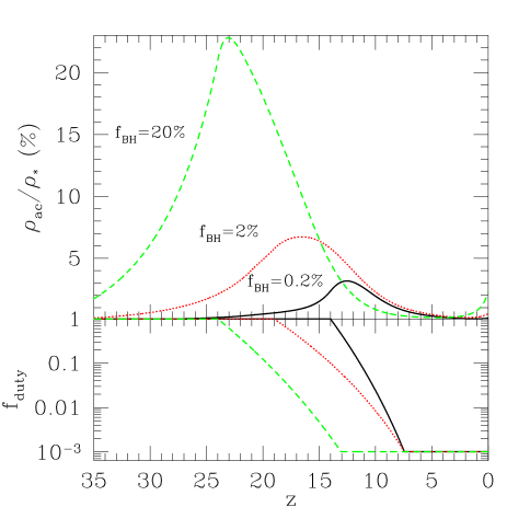
Figure 3: The top panel shows the mass fraction accreted onto seed BHs with respect to the star fraction in the universe. The bottom panel shows the duty cycle, $f_{\rm duty}$, assumed in each model. The solid, dotted and dashed lines refer models M3, M4, and M5 in table 2, respectively.

Finally, in Fig. 3, we show the mass fraction accreted onto seed BHs with respect to the star fraction in the universe, $\rho_{\rm ac}/\rho_{*}=\omega_{\rm ac}/\omega_{*}$ (top panel), and the adopted duty cycle (bottom panel). Again, the dashed, dotted and solid lines refer to models M3, M4 and M5 in table 2. As shown by the labels next to each line, the early accretion model has $f_{\rm BH}=20$%, therefore it requires that most of the mass of Population III stars implodes into BHs. But for the other models only a fraction $f_{\rm BH}\lower 2.15277pt\hbox{$\;\buildrel<\over{\sim}\;$}2$% of the stars needs to implode into BHs. This condition does not require a top-heavy IMF. It is interesting to note (but not surprising) that in order to have a substantial mass accretion onto seed BHs at early times a large fraction of seed BHs, $f_{\rm BH}$, from Population III stars is required. This is because the accreted mass increases exponentially with e-folding time scale $t_{\rm Ed}\simeq 10^{8}$ yrs, which is about the Hubble time at $z=30$. To conclude we note that if seed BHs are not able to accrete initially at the Eddington rate (see bottom panel of Fig. 3 that shows the adopted duty cycle), a larger fraction of seed BHs, $f_{\rm BH}$, is necessary in order to get the same global accretion rate as in our models. This is clearly possible to do for the intermediate and late accretion models, but would need extremely high and unrealistic values of $f_{\rm BH}$ in the early accretion model M3.

3.1 Spectral Energy Distribution

In Fig. 4 we show the spectral energy distribution (SED) of stars and quasars adopted in our simulations. For the stars we adopt a SED calculated for zero-metallicity stars (Tumlinson & Shull, 2000) and for quasars we use a spectrum similar (but not identical) to the one calculated by Sazonov et al. (2004). Their spectrum is a template, inferred on the basis of observations, representing the average quasar in the universe and determined by considerations both of the (X, $\gamma$) ray background and the spectra of individual objects. The quasar spectrum has an X-ray bump produced by absorption of UV photons by intervening gas and an IR excess produced by the reprocessed UV photons. Using this SED we can distinguish between reionisation by UV photons produced mainly by the stars and X-rays produced by quasars. The energy band that contributes the most to reionisation, also amplified by the effect of secondary electrons, is 0.5 keV $<h_{p}\nu<5$ keV. But as we will point out in paper IIb, the X-ray background photons that are redshifted to the extreme ultraviolet (EUV) bands can be the dominant source for preionisation in the voids.

The typical expected mass of the accreting BHs in our model is $M_{\rm BH}\lower 2.15277pt\hbox{$\;\buildrel<\over{\sim}\;$}100-1000$ M_⊙ at the high redshifts of interest, while the adopted SED is inferred from the accretion onto BHs with masses of $M_{\rm BH}\lower 2.15277pt\hbox{$\;\buildrel<\over{\sim}\;$}10^{5}-10^{6}$ M_⊙. Generally speaking the SED of accreting compact objects has two components that contribute comparably to the total energy output: (i) a power law component from the hot corona around the BH and (ii) a thermal component from the inner part of the hot accretion disk. The power law component is independent of the mass of the accreting object (from X-ray binaries to AGN) while the disk component has a temperature that depends mildly on the mass of the BH as $kT_{\rm disk}\approx 1.2~{}{\rm keV}(M_{\rm BH}/10~{}{\rm M}_{\odot})^{-1/4}$. The observed spectra of ULX sources tentatively show a subdominant soft component fitted by multicolour disks blackbody with $kT_{\rm disk}\sim 0.15$ keV, which has been interpreted as a tentative evidence of intermediate mass black holes (Miller et al., 2003). The non-thermal component, which dominates the total energy output, is a power law similar to the one adopted in the present paper. Note that the spectrum that we have assumed is also similar to the Sazonov et al. (2004) “absorbed quasar spectrum” (Fig. 4) were the UV bump produced by the thermal component in supermassive BHs is absorbed and in fact has no UV at all. The spectrum that we adopt is therefore dominated by the power law component (absorbed in the UV) that is roughtly independent of the assumed mass of the accreting BH.

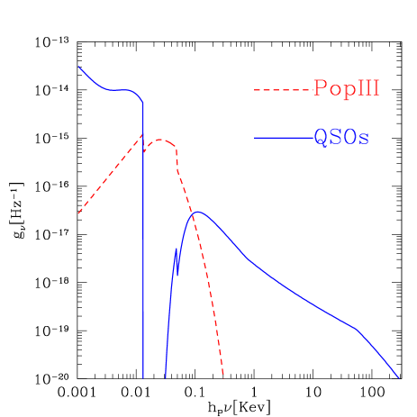
Figure 4: Spectral energy distribution of Population III stars (dashed line) and quasars (solid line). UV radiation is mainly emitted by stellar sources and X-rays by quasars. We assume that most UV radiation from quasars does not escape to the IGM but it is absorbed by an obscuring torus or in the ISM. In the adopted quasar SED the thermal component, that depends mildly on the BH mass, is negligible with respect to the power low component that is mass independent.

4 Semianalytic Models

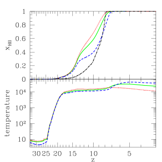
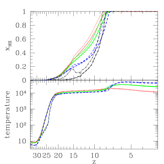
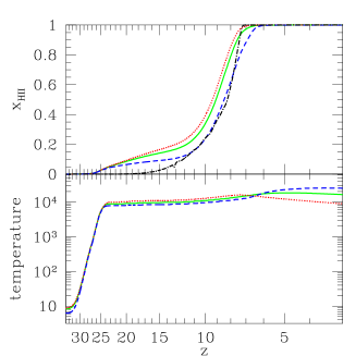
Figure 5: (left) The top panel shows the ionised hydrogen fraction and the volume filling factor of H ii regions (dot-dashed line) as a function of redshift for model M3. The bottom panel shows the IGM temperature as a function of redshift for model M3. The dotted, solid and dashed lines refer to gas over-densities $\delta=0.1,1,10$ in the IGM outside H ii regions, respectively. After overlap, when the ionising background is uniform, the lines refer to the ionised IGM. (centre) Same as in the left figure but for model M4 (thick lines) and M4b (thin lines). (right) Same as in the left figure but for model M5.

In this section we show the results found using a semianalytic model for reionisation. The advantage of the semianalytic approach with respect to the cosmological simulations presented in paper IIb is that we can explore a larger parameter space and the results are not affected by the resolution of the simulations. We use this approach to study the dependence of the Thomson optical depth on cosmological parameters and accretion histories of seed BHs. The results presented in this section also helped to derive a physically motivated, time dependent X-ray emissivity, to be used in the more computationally expensive numerical simulations. In addition, the semianalytic models are an aid for the interpretation of the results of cosmological simulations, made complicated by the interplay of a larger number of physical processes. If not otherwise specified, we adopt the concordance $\Lambda$CDM cosmological model with $h=0.72$, $\Omega_{\rm m}=0.27$, $\Omega_{\rm b}=0.046$, $n_{\rm s}=1$ and $\sigma_{8}=0.91$, that is consistent with the WMAP measurements ($h=0.71^{+0.04}_{-0.03}$, $\Omega_{\rm m}h^{2}=0.135^{+0.008}_{-0.009}$, $\Omega_{\rm b}h^{2}=0.0224\pm 0.0009$, $n_{\rm s}=0.93\pm 0.03$ and $\sigma_{8}=0.84\pm 0.04$, Spergel et al., 2003).

4.1 The code

We implemented a semianalytic model to study IGM reionisation, chemical evolution and re-heating. The filling factor of H ii regions is calculated following the method in Chiu & Ostriker (2000). But we also include X-ray ionisation of the IGM before overlap of the H ii regions. A detailed description of the code is given in Appendix A. Here we summarise the main processes included in the code at this stage:

• We calculate the mass function of DM haloes and the formation rate of haloes using the extended Press-Schechter formalism. The star formation rate (SFR) is proportional to the formation rate of haloes. In the integral for the global SFR we take into account cooling and dynamical biases that depend on the mass of the haloes.

• We include thermal feedback on star formation: the minimum mass of star-forming galaxies at a given redshift is determined by the IGM filtering mass.

• The emissivity of accreting BHs is calculated as in § 3.

• We assume a two-phase IGM. One phase is the fully ionised gas inside the H ii regions and the other is the partially-ionised or neutral gas outside the H ii regions.

• Radiative transfer is solved by splitting the spectrum into H i optically thick radiation and background radiation. Given the clumping factor inside H ii regions we follow the evolution of the filling factor, temperature and chemistry of the ionised gas. Outside the H ii regions the temperature and element abundances are calculated as a function of the overdensity.

• We calculate the time-dependent chemical network for 8 ions (H, H⁺, H^-, H₂, H${}_{2}^{+}$, He, He⁺, He⁺⁺) and thermal evolution inside and outside H ii regions. The following heating and cooling processes are included: collisional and photo-ionisation, ionisation by secondary electrons, H, He and H₂ cooling, Compton cooling-heating and the cosmological expansion term. We neglect cooling from metal contamination in small-mass galaxies. The rates are from Ricotti et al. (2001).

4.2 Results

We have run several models to study the sensitivity of the results to the accretion history on seed BHs and to cosmological parameters. In table 2 we list the parameters of the models shown in the next figures. In all the models the integrated energy emitted by accreting BHs is the same and stellar reionisation happens at $z\sim 7$. We normalise the BH accretion rate assuming that the total mass in BHs at $z=0$ is $\omega_{\rm BH,max}=10^{-4}$, the mass of SMBHs in the galactic centres. This assumption is rather conservative since it is likely that a fraction of seed BHs is not incorporated into the SMBH population at $z=0$. During galaxy mergers there is a non-negligible probability that one of the two merging BHs sitting in the bulge is expelled from the galaxy (cf., Madau et al., 2004). This probability is larger for unequal mass BHs, and happens in the final phase of the merger during the phase where gravitational radiation is emitted.

In summary the constraints on the semianalytic models are the following:

• The integrated energy output from accreting BHs is limited by assuming that the total mass in BHs at $z=0$ equals the total mass of SMBHs in the observed in the centres of galaxies. This requirement is a very conservative one, since theoretical calculations (e.g., Madau & Rees, 2001) show that most intermediate mass BHs formed at high redshift will not merge into the SMBHs in the galactic centres.

• Seed BHs accrete initially at the Eddington rate. The duty cycle in the late preionisation model (M3) is consistent with observations of QSO at $z\sim 3$ that show a duty cycle of 3% and with QSO at $z\sim 0$ that show a duty cycle of 0.1%

• The star formation efficiency is constrained by fitting the observed star formation rate (Madau plot) at $z<6$ (Lanzetta et al., 2002). The integrated baryon fraction in stars at $z=0$ is consistent with the one estimated by Fukugita et al. (1998).

• The effective UV emissivity from stellar sources is constrained to reproduce the transmitted flux observed in the Sloan quasars at $z<6.2$. Assuming a Salpeter IMF the adopted escape fraction is $\langle f_{\rm esc}\rangle$ $=30$ %.

• The specific intensity of the ionising background at $z<6$ is consistent with observations.

The typical ionisation and thermal history of the X-ray preionisation scenario is illustrated in Fig. 5 for hydrogen and Fig. 6 for helium. In Fig. 5 we show the hydrogen ionisation (top panel) and the IGM thermal history (bottom panel) for model M3 (figure on the left), model M4 and M4b (figure in the centre) and for model M5 (figure on the right). In model M3, BH accretion takes place mostly at $z>15$, at $z>20$ in model M4, and at $z>25$ in model M5. The dotted, solid and dashed lines refer to gas over-densities $\delta=0.1,1$, and 10, respectively. Before reionisation at $z_{\rm rei}$ $\sim 7$, the lines refer to the gas outside the H ii regions. After overlap, when the ionising background is uniform, the lines refer to the fully ionised IGM. The dot-dashed lines in the top panels show the volume filling factor of the H ii regions as a function of redshift. In the figure at the centre the thin lines show a model (M4b) where the UV emissivity is about 10 times larger at $z>15$ than at $z<15$, to account for the contribution of a top-heavy Population III star population. The volume filling factor of the H ii regions in this model differs from the same model where the Population III contribution is neglected (M4). The optical depth to Thompson scattering in model M4 and M4b has about the same value.

As even the earliest investigations showed (Ostriker & Gnedin, 1996), reheating significantly precedes reionisation (weather or not X-ray ionisation is included). In any X-ray preionisation model, by the time the ionisation fraction in the IGM reaches $\langle x_{\rm e}\rangle$ $\sim 10$%, the IGM has a temperature $T\approx 10^{4}$ K (cf., Fig. 5). This happens in all the models independently of the starting redshift of preionisation because the ionising efficiency of secondary electrons is reduced when $\langle x_{\rm e}\rangle$ $\lower 2.15277pt\hbox{$\;\buildrel<\over{\sim}\;$}10$% and the energy of X-ray photons is mostly converted into heat.

By inspecting the dotted, solid, and dashed lines in the bottom panels of Fig. 5, that show the gas temperature at overdensities $\delta=0.1,1$, and 10, respectively, we identify three epochs in the reheating history of the IGM. Initially, before complete reionisation by UV radiation, the temperature of the IGM outside the cosmological H ii regions is almost isothermal ($T_{\rm IGM}\approx 10^{4}$ K) with overdense regions slightly cooler than underdense regions . At reionisation the IGM becomes isothermal. After reionisation the IGM temperature dependence on the density follows a tight relationship, often referred to as “the effective equation of state of the IGM”, $T_{\rm IGM}=T_{\rm IGM,0}(1+\delta)^{(\gamma-1)}$, where $\delta$ is the overdensity (Hui & Gnedin, 1997). The parameter $(\gamma-1)$ is zero (i.e., the IGM is isothermal) at reionisation and $(\gamma-1)>1$ (i.e., overdense regions are hotter than the mean density gas) after reionisation. The temperature $T_{\rm IGM,0}$ at reionisation is determined by the spectrum of the background radiation: it is higher the harder the spectrum. If the spectrum does not evolve afterwards, the temperature of the IGM is expected to decrease almost adiabatically (e.g., $(\gamma-1)\sim 0.6$).

In our models the adopted spectrum at $z_{\rm rei}=7$ is consistent with the temperature and $(\gamma-1)$ at $z=3-5$ derived from the line widths of the Lyman-$\alpha$ forest: $T_{\rm IGM,0}\sim 1-3\times 10^{4}$ K, $(\gamma-1)\sim 0.1-0.4$ (Ricotti et al., 2000; Schaye et al., 2000; Theuns et al., 2002). We find that the IGM temperature decreases slowly with redshift ($T_{\rm IGM}\propto(1+z)^{0.5}$) and the equation of state has $(\gamma-1)=0.3\pm 0.1$ (i.e., an intermediate value between the isothermal and adiabatic case). Loose constraints (due to the large errors on the measured temperature) can be put on reionisation models using the observed $T_{\rm IGM}$. If reionisation happens too early and the IGM is not reheated by additional sources that produce the hardening of the background spectrum, the temperature at $z\sim 3-5$ would be too low when compared to observations. Or, if the spectrum is extremely hard at $z_{\rm rei}\simeq 7$, the IGM temperature at $z\simeq 3-5$ would be higher than observed. Compton heating is always much less efficient than photoionisation heating in these models. We have estimated that it is subdominant if the neutral fraction is $x_{{\text{H\,\sc i}}}\lower 2.15277pt\hbox{$\;\buildrel>\over{\sim}\;$}10^{-7}$.

In Fig. 6 we show the He ionisation history for model M3. The dotted, solid and dashed lines refer to gas over-densities $\delta=0.1,1$, and 10, respectively. Interestingly, in this model (and in model M4) the He ii was almost fully reionised at high-z and fully reionised at $z\sim 3$. Helium double ionisation is almost complete at $z\sim 15$ but afterwards He ii recombines very slowly as the X-ray emissivity decreases. Note that the recombination rate of He iii is four times faster than the one of H ii . The reason for this slow recombination rate of He iii is the following. In this model the second reionisation of He ii it is not produced by a second peak in the X-ray emissivity at $z\sim 3$ due to AGN activity. Instead it can be explained by the hardening of the spectrum of the background radiation in the UV bands, that it is produced by the combination of two effects: (i) the IGM becomes increasingly transparent to ionising radiation after H i reionisation at $z_{\rm rei}=7$ and (ii) the background soft X-rays are redshifted into the hard-UV bands and ionise more efficiently the He ii . This effect is a general feature of all late and intermediate accretion models. This is illustrated in Fig. 7) that shows the effect of the redshifted background on the evolution of the He i and He ii photoionisation rates, $\Gamma$. Neglecting recombinations and the Hubble expansion we have approximately that $(t_{H}/n(He))dn(He)/dt\sim t_{H}\Gamma$, where $t_{H}$ is the Hubble time. The solid lines show $t_{H}\Gamma({\text{He\,\sc ii}})$ for He ii and the dashed lines $t_{H}\Gamma({\text{He\,\sc i}})$ for He i as a function of redshift. The thick lines refer to model M3 and the thin lines to model M4.

Observations of the He ii Lyman-$\alpha$ forest (e.g., Reimers et al., 1997; Theuns et al., 2002) and the line widths of the H i Lyman-$\alpha$ forest (Ricotti et al., 2000) at $z\sim 3$ suggest that He ii reionisation happens at redshift $z\simeq 3$. This is usually attributed to the observed peak of AGN activity at that redshift, but as noted in Miniati et al. (2004), heating from shocks arising from cosmic structure formation also can make a significant contribution. The scenario presented here is another available mechanism that can explain the observed He ii reionisation at $z\sim 3$ and is consistent with the redshift evolution of IGM equation of state. Note that in our models the temperature decreases slowly, monotonically, but does not show any substantial increase corresponding to the redshift of He ii ionisation at $z\sim 3$. The same smooth behaviour is exhibited by the parameter $(\gamma-1)$.

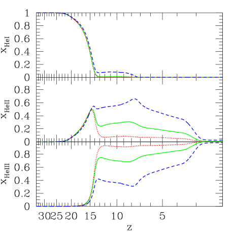
Figure 6: Helium ionisation history for model M3. The dotted, solid and dashed lines refer to gas over-densities $\delta=0.1,1$, and 10, respectively.

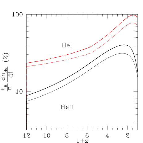
Figure 7: Effect of the redshifted background on the evolution of the He i (dashed lines) and He ii (solid lines) photoionisation rates, $\Gamma$. The lines show $(t_{H}/n(He))dn(He)/dt\sim t_{H}\Gamma$, where $t_{H}$ is the Hubble time, for model M3 (thick lines) and model M4 (thin lines).

The evolution of the SFR for models M3, M4 and M5 was shown in Fig. 2. Note that in model M5, in which BH accretion starts earlier, the thermal feedback strongly suppresses star formation in the smaller mass galaxies. This effect reduces the number of seed BHs and therefore the emission of X-rays at high redshift. The filling factor of H ii regions (shown in the top panels of Fig. 5) has an evolution similar to that of the SFR: after the initial growth, the filling factor remains constant at a few percent of the volume. It starts growing again when most massive galaxies form at $z\sim 15$. This effect is also observed in the cosmological simulations with radiative feedback discussed in paper IIb.

The optical depths to Thomson scattering produced by the X-ray preionisation models are within the 65% confidence limit of WMAP. The models are also in agreement with $\tau_{\rm e}$ $\sim 0.103^{+0.060}_{-0.047}$ found by Tegmark et al. (2003) by combining WMAP and other CMB experiments with the Sloan Digital Sky Survey (see their Table 4). The optical depth, $\tau_{\rm e}$, and the visibility function $g(z)=e^{-\tau_{\rm e}}d\tau_{\rm e}/d\eta$ (where $\eta$ is the conformal time) as a function of redshift for models M3, M4, and M5 are shown in Fig. 8. The three models differ for the accretion history onto seed black holes. In model M5 most of mass in black holes is accreted at $z>25$, in model M4 at $z>20$ and in model M3 at $z>15$. It is interesting that model M4 has the larger $\tau_{\rm e}$, even if all the models have the same integrated energy input from accreting BHs. This is due to the small, but non-negligible, recombination rate of partially ionised gas. If the IGM is partially ionised at high redshift and recombinations can be neglected, $\tau_{\rm e}$ should increase the earlier the partial ionisation begins, and vice-versa if the partial ionisation starts later. But if recombinations are not negligible at high redshift, then there is an intermediate redshift that maximises $\tau_{\rm e}$. In our models this redshift is $z\sim 15$ (model M4).

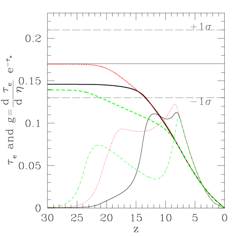
Figure 8: Thomson scattering optical depth, $\tau_{\rm e}$, and visibility function, $g(z)$, as a function of redshift. Models M3 (solid lines), M4 (dotted lines) and M5 (dashed lines) are shown. The models differ for the accretion history of BH seeds (duty cycle) but have the same total integrated X-ray energy input. The maximum of $\tau_{\rm e}$ is obtained for model M4, that has the bulk of accretion at intermediate redshift ($z\sim 20$) with respect to models M3 and M5.

Another interesting effect worth noticing is the delay between the formation of the first sources and the build-up of a substantial background. Roughly the time scale for building the background is given by a fraction of the Hubble time. For instance, if the first sources formed at $z=40(30)$, the X-ray background will build up at $z=25(20)$. Also, as already noted, the age of the universe at $z=30$ is about one Eddington time $t_{\rm Ed}=10^{8}$ yr. If seed BHs accrete at the Eddington limit their mass would grow exponentially one e-folding from $z=30$ to $z=20$ and 4 e-foldings to $z=12$. Therefore, the energy available to produce X-rays in the very early universe is limited to 5-10 times the mass of the seed BHs. This means that we need an increasingly large mass in seed BHs to preionise the IGM starting at higher redshift (cf., Fig. 3). This is only possible if the IMF of the first stars is top-heavy and has been discussed in paper I.

To illustrate the effect of cosmological parameters on the $\tau_{\rm e}$ produced by X-ray preionisation, in Fig. 9 we show $\tau_{\rm e}$ and $g(z)$ for model M3b that has a spectral index of initial density perturbations $n_{\rm s}=1.04$ and, for comparison, model M3 that has $n_{\rm s}=1$ normalised to the same amplitude of the power spectrum at $k=0.05$ h Mpc^-1 measured by WMAP (Verde et al., 2003). The other parameters in model M3b and M3 are the same. In model M3b seed BHs form earlier and the preionisation starts at higher redshift than in model M3. In this model we get $\tau_{\rm e}$ $=0.16$, compared to $\tau_{\rm e}$ $=0.14$ of model M3. This result is qualitatively different if reionisation is instead produced by UV sources. In this second case, in paper I we have shown that $\tau_{\rm e}$ is not substantially increased if the power spectrum of initial perturbations has more power on small scales because star formation in small mass galaxies is regulated and limited by feedback effects.

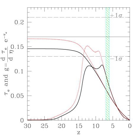
Figure 9: As in Fig. (8) for model M3 with spectral index of primordial perturbations $n_{\rm s}=1$ (solid lines) and the same model but using $n_{\rm s}=1.04$ (model M3b, dot-dashed lines).

Table 3: Results of the semianalytic models

Model	$\tau_{\rm e}$	$z_{g}^{max}$	$y$-par	${\omega_{\rm BH}\over\omega_{*}}$	$f_{\rm XRB}$	$\Gamma({\text{He\,\sc ii}})t_{\rm H}$
			$\times 10^{7}$	(%)	(%)	(%)
M3	0.146	12.0	$3.64$	3	5 (12)	35
M3b	0.166	12.5	$4.26$	3	5 (12)	35
M4	0.170	17.0	$3.95$	9	7 (17)	25
M4b	0.170	17.0	$3.95$	9	7 (17)	25
M5	0.140	21.5	$2.96$	42	0.3 (1)	1.5

Meaning of the values in each column: $\tau_{\rm e}$ is the Thomson scattering optical depth; $z_{g}^{max}$ is the high-redshift maximum of the visibility function $g(z)$; $y$ is the Compton distortion parameter; $\omega_{\rm BH}/\omega_{*}$ is the maximum ratio of BH to stellar cosmic density (to translate $\omega_{\rm BH}$ to $\rho_{\rm BH}$ multiply by $5.5\times 10^{9}$ M_⊙ Mpc${}^{-}3$); $f_{\rm XRB}$ is the fraction of the X-ray background at 50-100 keV (and 2-10 keV, in parenthesis) due to early black holes; $\Gamma({\text{He\,\sc ii}})t_{\rm H}\sim(t_{H}/n_{{\text{He\,\sc ii}}})dn_{{\text{He\,\sc ii}}}/dt$ is the fractional rate of He ii photoionisation per Hubble time per helium atom due to the redshifted X-ray background.

In conclusion, adopting the model constraints listed at the beginning of this section, we obtain values of $\tau_{\rm e}$ consistent with WMAP. The models are consistent with and do not violate any observation at $z<6$ that are evident. In the following paragraphs we discuss a few obvious observational constraints. But we will focus and return to this discussion in paper IIb.

Reheating of the IGM at redshifts $z<10^{5}$, produces a Comptonised spectrum of the CMB blackbody. The Compton distortion is usually parametrised by the value of the $y$:

$$y\equiv\int_{0}^{\tau_{e}^{\rm max}}{k_{\rm B}(T_{e}-T_{\rm CMB})\over m_{e}c^{2}}d\tau_{e}\simeq 1.7\times 10^{-6}\int_{0}^{\tau_{e}^{\rm max}}{T_{e}\over 10^{4}K}d\tau_{e},$$

where $T_{e}$ is the electron temperature, $T_{\rm CMB}$ is the CMB photon temperature and $\tau_{e}$ is the optical depth to electron Compton scattering. An upper limit on the $y$-parameter $y\lower 2.15277pt\hbox{$\;\buildrel<\over{\sim}\;$}1.5\times 10^{-5}$ at 95% CL has been determined using COBE satellite data (Fixsen et al., 1996). The maximum value of $y$ that we find in our models, $y\simeq 4\times 10^{-7}$, is not constrained by the current data on the spectral distortion. A future experiment with an upper limit on the $y$-parameter improved by two orders of magnitude would be able to detect a possible X-ray preionisation and reheating in the early universe.

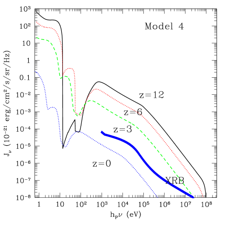
Figure 10: Background radiation at $z=12,6,3$ and $z=0$ for model M4. The thick line shows the X-ray background radiation at $z=0$ (Comastri et al., 1995). The redshifted X-ray background produced by early epoch of black hole accretion constitutes about $5-10$% of the hard X-ray background in the 2-50 keV bands.

In Fig. 10 we show the background radiation at $z=12,6,3$ and $z=0$ for model M4. The thick line shows the X-ray background radiation at $z=0$ (Comastri et al., 1995). We see that the redshifted X-ray background produced by early epoch of black hole accretion constitutes about $5-10$% of the hard X-ray background in the 2-50 keV bands.

The observed (X,$\gamma$) ray background is produced almost completely by known sources (mainly Seyfert galaxies at $z\sim 1-2$). However there is some room for additional sources and recently De Luca & Molendi (2004) have estimated that that about 20% of the observed background may be produced by a new population of faint X-ray sources, currently undetected within the sensitivity limits of the deepest X-ray surveys. The intensity of the high redshift X-ray background decreases from its value at redshift $z$ as $(1+z)^{-3+\phi}$, where $\phi$ is the logarithmic slope of the spectral energy distribution. By imposing that the redshifted background produced at the redshift of the peak of the BH accretion does not exceed 20% of the observed value at $z=0$ we find the following upper limit for the BH accretion rate:

$$\dot{\rho}_{\rm ac}^{\rm max}\lower 2.15277pt\hbox{$\;\buildrel<\over{\sim}\;$}(10^{-2}M_{\odot}{\rm Mpc}^{-3}{\rm yr}^{-1})\left({0.1\over\beta}\right)\left({1+z\over 20}\right)^{-3.7}.$$ (11)

Note that we this expression has been derived for the accretion history of the models presented in the present paper. It implicitly assumes that $\dot{\rho}_{\rm ac}=\Delta\ rho_{\rm ac}/\Delta t$ with $\Delta t\simeq t_{H}(z)$, where $t_{H}(z)$ is the Hubble time at the redshift of maximum accretion (i.e., the accretion rate rapidly fades after the maximum).

In table 3 we summarise the values of some relevant quantities computed from the semianalytic models listed in table 2. See the table footnote for the explanation of the meaning of the quantities shown in each column of the table.

5 Discussion and Summary

In a previous paper (paper I), we showed that even with a top heavy mass function Population III stars could not reionise the universe to a significant degree if they end their lives as pair instability supernovae. The reason is that such events contaminate the high density regions to such an extent that further formation of extremely low metallicity stars becomes impossible before significant ionisation has occurred. But, if these same stars implode to massive black holes, then accretion onto them at near Eddington rates will produce a pervasive X-ray background which can quite efficiently partially preionise the bulk of the cosmic baryons before $z=15$ and give an optical depth to Thompson scattering (cf., table 3) consistent with WMAP results. The primary reason for the increased efficiency is the long mean free path of X-rays which both increases the fraction of photons that escape the parent halo and ionises preferentially in the low density regions where recombination rates are low. In addition X-rays only partially ionise the IGM to 10-20%, therefore the recombination rate is reduced with respect to the reionisation scenario produced by UV sources. Thus we find that the average number of times a baryon is photoionised in this picture is about unity for $\tau_{\rm e}$ $\simeq 0.15$ while it is about ten in the case when stellar UV is used (paper I). Moreover, since the X-rays preionise the low density regions of the IGM at early times, the required number of ionising photons from Population II stars to have reionisation at redshift $z\simeq 6$ is much reduced.

But we might ask, could the X-rays arise as easily from X-ray binaries or could SN remnants (cf., Oh, 2001)? These other sources are certainly helpful but they will generate somewhat less energy in X-rays than accretion can do. The ratio of X-ray energy to massive star formation expressed as an efficiency is $\epsilon_{\rm SN}=E_{51}10^{51}{\rm erg}/143M_{\odot}c^{2}\sim 4\times 10^{-6}$ for these sources (assuming Population II with Salpeter IMF and neglecting Compton cooling of the X-ray emitting hot gas) but we see from $\epsilon_{\rm ac}=0.15\beta(M_{\rm SMBH}/M_{\rm bulge})$ that the comparable number from accretion is $2.25\times 10^{-5}$.

What are the observable consequences of the scenario we are proposing (in addition to generating a large $\tau_{\rm e}$)?

1. The power spectrum of the cross correlation of temperature and polarisation of the CMB is sensitive to the visibility function $g(z)=e^{-\tau_{\rm e}}d\tau_{\rm e}/d\eta$ (cf., Fig. 8-9). The Planck satellite should be able to distinguish between the visibility function produced by an early X-ray partial ionisation (peaking at large z) or the one expected for reionisation by stellar sources (peaking at lower z).

2. Since the assumed spectrum (Fig. 4) has a positive slope $(d\ln L_{\nu}/d\ln\nu)>3$ for much of the relevant range of frequencies there are ever fresh ionising photons available and the probability per unit time that a neutral hydrogen atom is ionised does not decrease with time. This produce softer photons that, even if the ionisation efficiency of X-rays decreases when the ionisation fraction exceeds 10-20%, enhance the ionisation fraction in the voids to values larger than 20 % because of the contribution from the redshifted photons of the X-ray background. In most models, the photons from the redshifted X-ray background can fully reionise He ii at redshift $z\sim 3$ without any additional contribution from quasars at lower redshifts. Due to the heating rate by He ii ionisation the temperature of the mean density intergalactic medium remains close to $10^{4}$ K down to redshift $z\sim 1$ and the IGM equation of state has index $(\gamma-1)\sim 0.3$.

3. The maximum accretion rate onto seed black holes as a function of redshift is limited by the observed magnitude of the $\gamma$ ray background at $z=0$. This limits the ability of late preionisation models to produce large values of $\tau_{\rm e}$ and contribute substantially to the mass growth via accretion of seed black holes. In models that produce optical depth $\tau_{\rm e}$ $\sim 0.17$ consistent with WMAP, the redshifted X-ray background produced by the early epoch of black hole accretion constitutes about $5-10$% of the hard X-ray background in the 2-50 keV bands.

4. The model predicts that dwarf spheroidal galaxies, if they are preserved fossils of the first galaxies, would host a mass in black holes that is 5-40% of their stellar mass (cf., table 3). The larger values are produced in the early preionisation scenarios and it might be possible to rule them out on the base of observations from dynamical considerations.

5. The IGM is reheated to $T=10^{4}$ K before the ionisation fraction exceeds 10% producing typical values of the Compton distortion parameter $y\sim 4\times 10^{-7}$. The observational upper limit on this parameter is $y<1.5\times 10^{-5}$, too large to constrain our models. Star formation in the smaller mass haloes is reduced by the increase in the IGM Jeans mass following this early reheating.

6. The redshifted 21cm signal in emission and absorption against the CMB can be used to discriminate between preionisation scenarios and reionisation from UV sources. This will be discussed in paper IIb, where we will also show that preionisation by X-rays produces CMB secondary anisotropies on small angular scales that are easy to recognise when compared to models of inhomogeneous early reionisation by stellar sources with the same $\tau_{\rm e}$.

What are the requirements of the X-ray preionisation models in terms of seed black hole production from the first stars and accretion?

Since the time scale for accretion, $t_{\rm Ed}=10^{8}$ yr, is comparable to the Hubble time at $z=30$ the maximum X-ray emissivity at high-redshift is proportional to the total mass of the seed BHs. For this reason, in order to get a larger $\tau_{\rm e}$ in early preionisation scenarios, a top-heavy IMF is favoured over a Salpeter IMF. But this is true only if super-massive stars mostly end their lives collapsing directly into BHs without exploding as SNe or as pair-instability SNe.

We have shown models where the accretion onto seed black holes is near the Eddington rate at early redshift. This might perhaps be difficult to achieve. But it is worth noticing that it is not strictly necessary that the accretion is at the Eddington rate initially. Although, if the accretion rate is less efficient than that, a larger stellar mass fraction producing seed black holes, $f_{\rm BH}$, is needed to accommodate for this (see equation (8)).

In this paper we have explored a range of models with different accretion histories onto seed black holes. But we note that the models are not all equally plausible scenarios. The very early preionisation scenario (M5) is not the most favourable for several reasons: (i) as noted by Madau et al. (2004), accretion in small-mass haloes can be difficult because of the substantial gas photoevaporation in these galaxies (ii) if seed BHs do not accrete at near the Eddington rate the mass fraction, $f_{\rm BH}$, of seed BHs is extreme also assuming top-heavy Population III stars (iii) the number of recombinations per ionising photon in this model is larger than in the intermediate preionisation model and therefore $\tau_{\rm e}$ is reduced. The late preionisation model (M3) is also not favourable because it produces a low $\tau_{\rm e}$ if we constrain the maximum black hole accretion rate using equation (11) to be consistent with the observed $\gamma$-ray background at $z=0$. We therefore conclude that preionisation starting at $z\sim 15-20$ (e.g., model M4) is the most plausible scenario to reproduce $\tau_{\rm e}$ measured by WMAP. In this case $\sim 10$% of the X-ray background in the 2-50 keV band is produced by the early generation of mini-quasars and roughtly half of the currently estimated black hole mass density was formed at early times (even if only a fraction of them may have merged into the SMBHs in the galactic centres). In paper IIb we study this scenario using hydrodynamic cosmological simulations with radiative transfer and we discuss observations that could probe this model.

We also note in conclusion that this picture while consistent with the central values of WMAP results could not easily produce $\tau_{\rm e}$ at the upper end of the presently allowed values. If $\tau_{\rm e}$ $\lower 2.15277pt\hbox{$\;\buildrel>\over{\sim}\;$}0.2$, X-ray preionisation is not likely the dominant responsible mechanism and other scenarios need to be considered (e.g., decaying particles, non Gaussian perturbations, spectral index $n_{\rm s}>1$, primordial BHs, unconventional recombination).

ACKNOWLEDGEMENTS

MR is supported by a PPARC theory grant. Research conducted in cooperation with Silicon Graphics/Cray Research utilising the Origin 3800 supercomputer (COSMOS) at DAMTP, Cambridge. COSMOS is a UK-CCC facility which is supported by HEFCE and PPARC. MR thanks Martin Haehnelt and the European Community Research and Training Network “The Physics of the Intergalactic Medium” for support. The authors would like to thank Andrea Ferrara, Nick Gnedin, Martin Haehnelt, Piero Madau and Martin Rees for stimulating discussions and Mark Dijkstra for noticing some incorrect numbers in the first draft of this paper. MR thanks Erika Yoshino support.

Appendix A A Semianalytic Model for Reionisation

We implemented a semianalytic model to study reionisation, chemical evolution and re-heating of the IGM. The code is based on the method of Chiu & Ostriker (2000) for the calculation of the filling factor of ionised regions and for the star formation recipe. The main difference is the inclusion of radiative transfer for the background radiation that allows us to follow the thermal and chemical evolution of the IGM outside the H ii regions surrounding each UV source. We also consider the thermal feedback produced by the X-ray reheating of the IGM (see § A.4). The mass function of DM haloes and their formation/merger rates are calculated using the extended Press-Schechter formalism. The star formation rate is assumed to be proportional to the formation rate of haloes (see § A.1). We consider the IGM as a two-phase medium: one phase is the ionised gas inside the H ii regions and the other is the neutral or partially ionised gas outside. We solve the radiative transfer for the volume averaged specific intensity and we derive the specific intensity inside and outside the H ii regions from their volume filling factor and by separating the contribution from local UV sources and the background radiation from distant sources (see § A.3). We solve the time-dependent chemical network for eight ions and the thermal evolution as a function of the gas density outside the H ii regions. Given the clumping factor of fully ionised gas around the UV sources we evolve the filling factor, temperature and chemistry inside the H ii regions (see § A.2). The following heating and cooling processes are included: collisional- and photo-ionisation heating, ionisation by secondary electrons (see § A.2.1), H, He, H₂ cooling, Compton and adiabatic cosmological cooling. The rates are the same as the ones used in (Ricotti et al., 2001). For some test cases the results of the semianalytic code are in good agreement with the results of the cosmological simulations with radiative transfer presented in this paper and in Ricotti et al. (2002b).

A.1 Star Formation

We assume that stars and quasars form in virialised DM haloes. We use the extended Press-Schechter formalism to calculate the formation rate of bound DM haloes of a given mass $M_{\rm dm}$ at the time $t$. In general, given a probability distribution function (PDF) of density perturbations, $P(\nu)$, the DM comoving mass fraction of collapsed objects with mass between $M_{\rm dm}$ and $M_{\rm dm}+dM_{\rm dm}$ is given by $\Omega_{\rm ps}d\ln M_{\rm dm}=P(\nu)d\nu$, where

$$\int_{0}^{\infty}d\ln M_{\rm dm}\Omega_{\rm ps}=\int_{0}^{\infty}d\nu P(\nu)=1.$$

The comoving number density of collapsed objects $N_{\rm ps}=\Omega_{\rm ps}\rho_{0}/M_{\rm dm}$, where $\rho_{0}$ is the mean DM density at $z=0$, is given by

$$N_{\rm ps}dM_{\rm dm} = 2\rho_{0}P(\nu)\nu\Delta(M_{\rm dm})d\ln M_{\rm dm},$$ (12)

$$\nu = {\delta_{c}\over\sigma(M_{\rm dm})D(t)},$$ (13)

$$\Delta(M_{\rm dm}) = {d\ln\nu\over d\ln M_{\rm dm}}=-{d\ln\sigma(M_{\rm dm})\over d\ln M_{\rm dm}},$$ (14)

where $\sigma(M_{\rm dm})$ is the variance of the fluctuation on a scale $M_{\rm dm}$ linearly extrapolated to $z=0$, $\delta_{c}\approx 1.69$ is the linear overdensity for collapse of a top-hat perturbation and $D(t)$ is the linear growth factor. Here we use a Gaussian PDF $P=(2\pi)^{-1/2}\exp{(-\nu^{2}/2)}$, but the method has been applied by (Chiu & Ostriker, 2000) to non-Gaussian PDFs. With a similar procedure as in (Ricotti, 2002), we normalise the star formation efficiency by assuming that at $z=0$ a fraction of baryons $\omega_{*}=14$% has been converted into stars. The global SFR between redshift $0<z<5$ agrees within the errors with the observed global SFR (e.g., Lanzetta et al., 2002). As shown in § 3, a similar method of normalisation is applied to the BH accretion efficiency by assuming that at $z=0$ a fraction of baryons $\omega_{\rm BH}=10^{-4}$ is in black holes.

The formation rate of virialised objects, $\dot{N}_{\rm form}$, can be derived using the Press-Schechter formalism and calculating the rate of “destruction” of bound objects that are incorporated in larger haloes:

$$\dot{N}_{\rm form}=\dot{N}_{\rm ps}+\dot{N}_{\rm dest}.$$ (15)

As in Chiu & Ostriker (2000), we use a destruction probability $\phi(t)=\dot{N}_{\rm dest}/N_{\rm ps}=\dot{D}/D$ derived assuming that the destruction probability is scale-invariant (see Sasaki, 1994). It follows that the probability that an object formed at time $t_{f}$ exists at time $t$ is

$$p_{\rm surv}(t|t_{\rm f})=\int_{t}^{t_{\rm f}}dt\phi(t)={D(t)\over D(t_{\rm f})},$$ (16)

where $D(t)$ is the linear growth factor. At redshifts $z>1$, $p_{\rm surv}(t|t_{\rm f})=a(t)/a(t_{\rm f})$ for the concordance $\Lambda$CDM cosmology. From equation (15), recalling that $\dot{D}/D\approx\Omega^{0.6}(\dot{a}/a)$, it follows

$$\dot{N}_{\rm form}=-N_{\rm ps}{\nu\over P}{dP\over d\nu}\phi(t)=N_{\rm ps}\nu^{2}\Omega^{0.6}\left({\dot{a}\over a}\right),$$

where $d\ln P/d\nu=-\nu$ for a Gaussian PDF ($P\propto\exp{(-\nu^{2}/2)}$). The comoving number density of haloes at time $t$ that formed at time $t_{f}$ is given by

$$\dot{N}(M_{\rm dm},t_{f},t)dM_{\rm dm}dt_{\rm f}=\dot{N}_{\rm form}(M_{\rm dm},t_{f})p_{\rm surv}(t|t_{\rm f})dM_{\rm dm}dt_{\rm f}.$$

The emission rate per unit volume from the sources, often called the source function $\overline{S}(t)$, when expressed in dimensionless units ${\cal S}=\overline{S}(t)/(n_{H}h\nu_{0})$, where $h\nu_{0}=13.6$ eV and $n_{H}$ is the hydrogen mean number density, is given by

$$\begin{split}{\cal S}(t)=n_{0}^{-1}\int_{0}^{\infty}dM_{\rm dm}\int_{0}^{t}dt_{\rm f}\\ \times\Psi(M_{\rm dm},t_{\rm f})\dot{N}((M_{\rm dm},t_{f},t){\cal L}(M_{\rm dm},t_{\rm f},t).\end{split}$$ (17)

The function $\Phi(M_{\rm dm},t_{\rm f})$, defined in § A.4, is a step function that determines the minimum mass of forming galaxies as a function of the their time of formation, $t_{f}$. The dimensionless luminosity from each source is ${\cal L}_{\nu}\propto g_{\nu}\epsilon_{\rm UV}M_{*}c^{2}x\exp{(-x}/t_{\rm dyn})$, where $g_{\nu}$ is the SED of the source, $x=(t-t_{\rm f})/t_{\rm dyn}$ and $t_{\rm dyn}=(3\pi/32G\rho_{\rm vir})$ is the free-fall dynamical time.

A.2 Cooling and Chemistry

We solve the time-dependent equations for the photo-chemical formation/destruction of eight chemical species (H, H⁺, H^-, H₂, H${}_{2}^{+}$, He, He⁺, He⁺⁺), including the 37 main processes relevant to determine their abundances (Shapiro & Kang, 1987). We use ionisation cross sections from Hui & Gnedin (1997) and photo-dissociation cross sections from Abel et al. (1997). We solve the energy conservation equation

$${dE_{\rm gas}\over dt}=\Gamma-\Lambda,$$ (18)

where $E_{\rm gas}=(3kT/2)n_{H}(1+x(He)+x_{e})$, with $n_{H}$ the hydrogen number density, and $x(He)$ and $x_{e}$ the helium and electron fractions, respectively. Note that $n_{H}$ is a function of time because of Hubble expansion. Also, $x_{e}$ is time-dependent; neglecting this effect results in a temperature that is overestimated by about a factor of two. The cooling function, $\Lambda$, includes H and He line and continuum cooling (Shapiro & Kang, 1987), H₂ rotational and vibrational cooling excited by collisions with H and H₂ (Martin et al., 1996; Galli & Palla, 1998) and adiabatic cosmic expansion cooling. The heating term, $\Gamma$, includes Compton heating/cooling and photoionisation/dissociation heating. We solve the system of ODEs for the abundances and energy equations, using a $4^{\rm th}$-order Runge-Kutta solver. We switch to a semi-implicit solver (Gnedin & Gnedin, 1998) when it is more efficient (i.e., when the abundances in the grid are close to their equilibrium values). The spectral range of the radiation is between 0.7 eV and 10 keV. The primordial helium mass fraction is $Y_{P}=\rho(He)/\rho_{b}=0.24$, where $\rho_{b}$ is the baryon density, so that $x(He)=Y_{P}/4(1-Y_{P})=0.0789$. The initial values at $z=z_{i}$ for the temperature and species abundances in the IGM are: $T=10$ K, $x_{\rm H_{2}}=2\times 10^{-6}$, and $x_{e}\simeq x_{H^{+}}=10^{-5}/(h\Omega_{b}\Omega_{0}^{1/2})=6.73\times 10^{-4}$. The initial abundance of the other ions is set to zero.

Outside the Strömgren spheres surrounding the UV sources the thermal and chemical histories are calculated as a function of the gas density, using the specific intensity $\langle J_{\nu}\rangle_{\rm back}$ of the background radiation defined in § A.3.1. In this paper we show the abundances and the temperature of the IGM for three values of the baryon overdensity $\delta=\rho/\rho_{0}=0.1,1,10$. Inside the H ii regions we calculate the abundances of only H and He ions, since the abundances of molecular hydrogen and its ions are negligible, being photodissociated by H i ionising radiation. The effective coefficients of collisional ionisation and recombinations are larger by a factor $C_{{\text{H\,\sc ii}}}$, to take into account the gas clumping inside the H ii regions (see § A.3). The photoionisation and photoheating rates are calculated as shown in § A.2.1 using the specific intensity $J_{{\text{H\,\sc ii}}}$ of the radiation field inside H ii regions. The clumping factor $C_{{\text{H\,\sc ii}}}$ is tabulated as a function of redshift by fitting the clumping in the cosmological simulations with radiative transfer presented in paper IIb.

A.2.1 Secondary Ionisation and Heating from X-rays

Photoionisation of H i , He i , and He ii by X-rays and EUV photons produces energetic photoelectrons that can excite and ionise atoms before their energy is thermalised. This effect can be important before reionisation (Oh, 2001; Venkatesan et al., 2001), when the gas is almost neutral and the spectrum of the background radiation is hard due to the large optical depth of the IGM to UV photons.

Collisional ionisation and excitation of He ii by primary electrons are neglected since, in a predominantly neutral medium, they are unimportant. The primary ionisation rate for the species $i={\text{H\,\sc i}},{\text{He\,\sc i}},{\text{He\,\sc ii}}$ is,

$$\zeta^{i}=4\pi\int_{\nu_{i}}^{\infty}{J_{\nu}\over h_{p}\nu}\exp(-\tau_{\nu})\sigma_{\nu}^{i}d\nu,$$ (19)

where $\tau_{\nu}$ is the continuum optical depth, and $\sigma_{\nu}^{i}$ is the photoionisation cross section of the species $i$. Secondary ionisation enhances the photoionisation rates as follows:

$$\zeta_{s}^{{\text{H\,\sc i}}}=\zeta^{{\text{H\,\sc i}}}+\sum_{i={\text{H\,\sc i}},{\text{He\,\sc i}},{\text{He\,\sc ii}}}\zeta^{i}\langle\Phi^{{\text{H\,\sc i}}}(E_{0}^{i},x_{e})\rangle$$ (20)

$$\zeta_{s}^{{\text{He\,\sc i}}}=\zeta^{{\text{He\,\sc i}}}+\sum_{i={\text{H\,\sc i}},{\text{He\,\sc i}},{\text{He\,\sc ii}}}\zeta^{i}\langle\Phi^{{\text{He\,\sc i}}}(E_{0}^{i},x_{e})\rangle,$$ (21)

where $\langle\Phi^{{\text{H\,\sc i}}}(E_{0}^{i},x_{e})\rangle$ and $\langle\Phi^{{\text{He\,\sc i}}}(E_{0}^{i},x_{e})\rangle$ express the average number of secondary ionisation per primary electron of energy $E_{0}^{i}=h_{p}\nu-I^{i}$ weighted by the function $(J_{\nu}/h_{p}\nu)\exp(-\tau_{\nu})\sigma_{\nu}^{i}$. Here $I^{i}=h_{p}\nu_{i}$ is the ionisation potential for the species $i$.

The photoionisation heating rates for the species $i={\text{H\,\sc i}},{\text{He\,\sc i}}$ are given by,

$$\Gamma^{i}=4\pi\int_{\nu_{i}}^{\infty}{J_{\nu}\over h_{p}\nu}\exp(-\tau)\sigma_{\nu}^{i}E_{h}(E_{0}^{i},x_{e})d\nu.$$ (22)

Analytic fits to the functions $\Phi^{{\text{H\,\sc i}}},\Phi^{{\text{He\,\sc i}}}$ and $E_{h}$, based on the Monte Carlo results of Shull & van Steenberg (1985) are given in Appendix B in Ricotti et al. (2002a).

A.3 Radiative transfer

The evolution of the specific intensity $J_{\nu}$ [erg cm^-3 s^-1 Hz^-1 sr^-1 ] of ionising or dissociating radiation in the expanding universe, with no scattering, is given by the following equation:

$${\partial J_{\nu}\over\partial t}+{\partial\over\partial x^{i}}\left(\dot{x}^{i}J_{\nu}\right)-H\left(\nu{\partial J_{\nu}\over\partial\nu}-3J_{\nu}\right)=-k_{\nu}J_{\nu}+S_{\nu}.$$ (23)

Here, $x^{i}$ are the comoving coordinates, $H$ is the Hubble constant, $k_{\nu}$ is the absorption coefficient, $S_{\nu}$ is the source function, and $\dot{x}^{i}=cn^{i}/a$, where $n^{i}$ is the unit vector in the direction of photon propagation and $a=(1+z)^{-1}$ is the scale factor. The volume-averaged mean specific intensity is

$$\bar{J}_{\nu}(t)\equiv\langle J_{\nu}(t,\vec{x},\vec{n})\rangle_{V},$$ (24)

where the averaging operator acting on a function $f(\vec{x},\vec{n})$ of position and direction is defined as:

$$\langle f(\vec{x},\vec{n})\rangle_{V}=\lim_{V\rightarrow\infty}{1\over 4\pi V}\int_{V}d^{3}x\int d\Omega f(\vec{x},\vec{n}).$$ (25)

The mean intensity $\bar{J}_{\nu}(t)$ satisfies the following equation:

$${\partial\bar{J}_{\nu}\over\partial t}-H\left(\nu{\partial\bar{J}_{\nu}\over\partial\nu}-3\bar{J}_{\nu}\right)=-\bar{k}_{\nu}\bar{J}_{\nu}+\bar{S}_{\nu},$$ (26)

where, by definition, $\bar{S}_{\nu}\equiv\langle S_{\nu}\rangle_{V}$, and $\bar{k}_{\nu}\equiv\langle k_{\nu}J_{\nu}\rangle_{V}/\bar{J}_{\nu}$. In general, $\bar{k}_{\nu}$ is not a space average of $k_{\nu}$, since it is weighted by the local value of the specific intensity $J_{\nu}$. But when the mean free path of radiation at frequency $\nu$ is much larger than the characteristic scale of the problem (in our case the size of the computational box), we have $\bar{k}_{\nu}=\langle k_{\nu}\rangle_{V}$.

If we rewrite equation (26) in terms of the dimensionless comoving photon number density $n_{\nu}=(aL_{\rm box})^{3}4\pi\bar{J}_{\nu}/h_{p}$ where $L_{\rm box}$ is a spatial scale (in this paper we take it to be the comoving size of the computational box), and $h_{p}$ is the Planck constant, using substitutions $dt=(a^{2}/H_{0})d\tau$ and $\xi=\ln(\nu)$, equation (26) can be reduced to the following dimensionless equation:

$${\partial n_{\xi}\over\partial\tau}={1\over a}{da\over d\tau}{\partial n_{\xi}\over\partial\xi}-\alpha_{\xi}n_{\xi}+S_{\xi},$$ (27)

where $\alpha_{\xi}=a^{2}\bar{k}_{\nu}/H_{0}$ and $S_{\xi}=a^{5}L_{\rm box}^{3}4\pi\bar{S}_{\nu}/h_{p}H_{0}$. Using a comoving logarithmic frequency variable,

$$\bar{\xi}=\xi+\ln(a),$$ (28)

equation (27) can be reduced to

$${\partial n_{\bar{\xi}}\over\partial\tau}=-\alpha_{\bar{\xi}}n_{\bar{\xi}}+S_{\bar{\xi}},$$ (29)

which has the formal solution,

$$\begin{split}n_{\bar{\xi}}(\tau+\Delta\tau)=n_{\bar{\xi}}(\tau)\exp\left[-\int_{\tau}^{\tau+\Delta\tau}dt^{\prime}\alpha_{\bar{\xi}}(t^{\prime})\right]\\ +\int_{\tau}^{\tau+\Delta\tau}dt^{\prime}S_{\bar{\xi}}(t^{\prime})\exp\left[-\int_{t^{\prime}}^{\tau+\Delta\tau}d\tau^{\prime}\alpha_{\bar{\xi}}(\tau^{\prime})\right].\end{split}$$ (30)

We calculate equation (30) at each time step, $\Delta\tau$, of the simulation. The two integrals inside the square brackets on the right side of equation (30) can be solved analytically. We solve the third integral numerically.

A.3.1 Background radiation and radiation inside H ii regions

Two terms contribute to the volume averaged specific intensity in equation (30). The first term is produced by the background radiation from redshifted distant sources and the second term is produced by the local sources:

$$\bar{J}_{\nu}=\bar{J}_{\nu}^{\rm sour}+\bar{J}_{\nu}^{\rm back}.$$ (31)

If the emissivity of the sources is zero (${\cal S}=0$), it follows that $\bar{J}_{\nu}^{\rm sour}=0$. Only photons with a mean free path larger than the mean distance between the sources contribute to the background radiation, $\bar{J}_{\nu}^{\rm back}$.

If the volume filling factor of the Strömgren spheres surrounding the UV source is $f_{{\text{H\,\sc ii}}}$, we can rewrite the volume averaged specific intensity as the sum of the mean specific intensity inside the volume occupied by the H ii regions and the volume outside the H ii regions:

$$\bar{J}_{\nu}=\bar{J}_{\nu}^{{\text{H\,\sc ii}}}f_{{\text{H\,\sc ii}}}+\bar{J}_{\nu}^{\rm back}(1-f_{{\text{H\,\sc ii}}}).$$ (32)

From equation (31) and equation (32) we get,

$$\bar{J}_{\nu}^{{\text{H\,\sc ii}}}={\bar{J}_{\nu}^{\rm sour}\over f_{{\text{H\,\sc ii}}}}+\bar{J}_{\nu}^{\rm back}.$$ (33)

In order to derive the specific intensity, $\bar{J}_{\nu}^{{\text{H\,\sc ii}}}$, inside the Strömgren spheres we need to estimate their volume filling factor $f_{{\text{H\,\sc ii}}}$. We calculate the evolution of the filling factor of H ii regions following closely the method introduced by Chiu & Ostriker (2000). For the sake of completeness we show the equations that we solve to derive $f_{{\text{H\,\sc ii}}}$ in the next section.

A.3.2 Filling factor of H ii regions

In order to calculate $f_{{\text{H\,\sc ii}}}$ it is more convenient to introduce the porosity parameter, $Q(t)$, of the H ii regions defined by the relationship $f_{{\text{H\,\sc ii}}}=1-\exp{[-Q(t)]}$. The porosity $Q(t)$ offers the advantage that when $f_{{\text{H\,\sc ii}}}\ll 1$ we have $Q(t)\approx f_{{\text{H\,\sc ii}}}$ and when $f_{{\text{H\,\sc ii}}}\simeq 1$ we have $Q(t)\lower 2.15277pt\hbox{$\;\buildrel>\over{\sim}\;$}1$. The porosity of the H ii regions is given by

$$\begin{split}Q(t)=\int_{0}^{\infty}dM_{\rm dm}\int_{0}^{t}dt_{\rm f}\\ \times\Psi(M_{\rm dm},t_{\rm f})\dot{N}((M_{\rm dm},t_{f},t)V_{{\text{H\,\sc ii}}}(M_{\rm dm},t_{\rm f},t),\end{split}$$ (34)

where $V_{{\text{H\,\sc ii}}}=(4\pi/3)r_{{\text{H\,\sc ii}}}^{3}$ is the comoving volume filled by the Strömgren spheres, where $r_{{\text{H\,\sc ii}}}$ is their comoving radius. Comparing equation (17) to equation (34) we find the following relationship between the ionised volume per unit luminosity and the mean comoving luminosity density ${\cal S}$:

$${n_{0}V_{{\text{H\,\sc ii}}}\over{\cal L}(t)}={Q(t)\over{\cal S}(t)}.$$ (35)

The contribution of each source to the mean specific energy density, $E=4\pi\overline{J}_{\nu}/c$ is given by,

$$\begin{split}\overline{E}={1\over c}\int_{0}^{\infty}dM_{\rm dm}\int_{0}^{t}dt_{\rm f}\Psi(M_{\rm dm},t_{\rm f})\dot{N}(M_{\rm dm},t_{f},t)\int{dVL\over 4\pi(ar)^{2}}\\ ={1\over c}\int_{0}^{\infty}dM_{\rm dm}\int_{0}^{t}dt_{\rm f}\dot{N}(M_{\rm dm},t_{\rm f},t)Lr_{{\text{H\,\sc ii}}}a(t)^{-2}.\end{split}$$ (36)

Using equation (35) we find that, in dimensionless units ${\cal E}=\overline{E}/(n_{H}h\nu_{0})$, the mean UV energy density is

$$\begin{split}{\cal E}={a\over c}\left({3Q(t)\over 4\pi{\cal S}}\right)^{1/3}n_{0}^{-4/3}\int_{0}^{\infty}dM_{\rm dm}\int_{0}^{t}dt_{\rm f}\\ \times\Psi(M_{\rm dm},t_{\rm f})\dot{N}(M_{\rm dm},t_{\rm f},t){\cal L}^{4/3}(M_{\rm dm},t_{\rm f},t).\end{split}$$ (37)

The time evolution of the mean UV energy density is calculated solving the energy conservation equation,

$${d{\cal E}\over dt}={\cal S}-\left[\gamma{\dot{a}\over a}+x_{{\text{H\,\sc i}}}c\sigma_{e}n_{H}\right]{\cal E}-x_{{\text{H\,\sc ii}}}{df_{II}\over dt}.$$ (38)

We have assumed that the spectral energy distribution of the ionising radiation is $g_{\nu}\propto\nu^{-\gamma}$. Here $\sigma_{e}$ is the effective UV energy loss cross section, defined as $\sigma_{e}=(\Gamma_{\rm ph}+\Gamma_{\rm ion})/(4\pi\overline{J})$. The time derivative of the filling factor is $\dot{f}_{II}=(1-f_{II})\dot{Q}(t)$. The porosity parameter $Q(t)$ and the volume filling factor of the H ii regions are obtained solving equation (38) and equation (37).

A.4 Radiative Feedback

Feedback mechanisms on star formation are the most difficult part to implement using the semianalytic approach. The recipes used should be based on results of numerical simulations or scaling relations based on observations (such as the dependence of the mass to light ratio on the luminosity of galaxies). Analysing the simulations in Ricotti et al. (2002b), it appears that star formation is regulated by the interplay of several processes:

1. Internal feedback by UV radiation that produces photo-evaporative winds

2. Internal feedback by SN explosions

3. External (but local) feedback from UV radiation that regulates H₂ formation/destruction and cooling

4. Thermal evolution of the IGM: the IGM Jeans mass sets the minimum mass of galaxies forming at a given redshift.

In the semianalytic code, due to impossibility of modelling local external feedback processes, we only implement process (iv) which is global. We neglect the effects of internal feedbacks (i) and (ii).

Galaxies with mass smaller than the Jeans mass in the IGM cannot virialise because the pressure of the IGM prevents the gas from falling into their halo potential well. Therefore the formation rate of galaxies with masses $M_{\rm dm}<10^{8}$ M_⊙ is suppressed if the IGM is reionised or heated by X-ray or hard-UV background to $T\approx 10,000$ K. This process works together with H₂ destruction to suppress the formation of small-halo galaxies. If we take into account the finite time required for pressure to influence the gas distribution in the expanding universe, then the filtering mass, $M_{\rm F,IGM}$, which depends on the full thermal history of the IGM, provides a better fit to the simulation results than the Jeans mass, which instead depends on instantaneous values of the sound speed (Gnedin, 2000b). The filtering mass of the IGM is simply related to the Jeans mass by the relationship,

$$M_{\rm F,IGM}^{2/3}={3\over a}\int_{0}^{a}da^{\prime}M_{J}^{2/3}(a^{\prime})\left[1-\left({a^{\prime}\over a}\right)^{1/2}\right].$$ (39)

The Jeans mass is given by

$$M_{J}={4\pi\over 3}\overline{\rho}\lambda_{J}^{3},$$ (40)

where $\lambda_{J}=2\pi c_{s}t_{\rm ff}$ is the Jeans length, $t_{\rm ff}=(4\pi G\overline{\rho})^{-1/2}$ is the free-fall dynamical time and $c_{s}$ is the IGM sound speed.

We implement the feedback imposing a minimum galaxy mass $M_{\rm min}=M_{\rm F,IGM}(t_{\rm f})$ and computing the new SFR and the IGM temperature iteratively. Using a geometric mean for the temperature we make sure to achieve convergence. In practice we use a step-function kernel,

$$\Phi(M_{\rm dm},t_{\rm f})=\begin{cases}0,&\text{if $M_{\rm dm}<M_{\rm F,IGM}(t_{\rm f})$}\\ 1,&\text{if $M_{\rm dm}\geq M_{\rm F,IGM}(t_{\rm f})$},\end{cases}$$ (41)

any time we integrate over the mass function of DM haloes.

References

- Abel et al. (1997) Abel, T., Anninos, P., Zhang, Y., & Norman, M. L. 1997, New Astronomy, 2, 181
- Abel et al. (2000) Abel, T., Bryan, G. L., & Norman, M. L. 2000, ApJ, 540, 39
- Abel et al. (2002) Abel, T., Bryan, G. L., & Norman, M. L. 2002, Science, 295, 93
- Becker et al. (2001) Becker, R. H., et al. 2001, AJ, 122, 2850
- Bennett et al. (2003) Bennett, C. L., et al. 2003, ApJS, 148, 1
- Bromm et al. (2002) Bromm, V., Coppi, P. S., & Larson, R. B. 2002, ApJ, 564, 23
- Cen (2003) Cen, R. 2003, ApJ, 591, L5
- Chiu et al. (2003) Chiu, W. A., Fan, X., & Ostriker, J. P. 2003, ApJ, 599, 759
- Chiu & Ostriker (2000) Chiu, W. A., & Ostriker, J. P. 2000, ApJ, 534, 507
- Ciardi et al. (2003) Ciardi, B., Ferrara, A., & White, S. D. M. 2003, MNRAS, 344, L7
- Comastri et al. (1995) Comastri, A., Setti, G., Zamorani, G., & Hasinger, G. 1995, A&A, 296, 1
- De Luca & Molendi (2004) De Luca, A., & Molendi, S. 2004, A&A, 419, 837
- Djorgovski et al. (2001) Djorgovski, S. G., Castro, S., Stern, D., & Mahabal, A. A. 2001, ApJ, 560, L5
- Fan et al. (2003) Fan, X., et al. 2003, AJ, 125, 1649
- Fixsen et al. (1996) Fixsen, D. J., Cheng, E. S., Gales, J. M., Mather, J. C., Shafer, R. A., & Wright, E. L. 1996, ApJ, 473, 576
- Fukugita et al. (1998) Fukugita, M., Hogan, C. J., & Peebles, P. J. E. 1998, ApJ, 503, 518
- Galli & Palla (1998) Galli, D., & Palla, F. 1998, A&A, 335, 403
- Gebhardt et al. (2000) Gebhardt, K., et al. 2000, ApJ, 539, L13
- Gnedin (1998) Gnedin, N. Y. 1998, MNRAS, 294, 407
- Gnedin (2000a) Gnedin, N. Y. 2000a, ApJ, 535, 530
- Gnedin (2000b) Gnedin, N. Y. 2000b, ApJ, 542, 535
- Gnedin & Gnedin (1998) Gnedin, N. Y., & Gnedin, O. Y. 1998, ApJ, 509, 11
- Haehnelt et al. (1998) Haehnelt, M. G., Natarajan, P., & Rees, M. J. 1998, MNRAS, 300, 817
- Haiman & Holder (2003) Haiman, Z., & Holder, G. P. 2003, ApJ, 595, 1
- Haiman et al. (1997) Haiman, Z., Rees, M. J., & Loeb, A. 1997, ApJ, 476, 458
- Heger & Woosley (2002) Heger, A., & Woosley, S. E. 2002, ApJ, 567, 532
- Hui & Gnedin (1997) Hui, L., & Gnedin, N. Y. 1997, MNRAS, 292, 27
- Kogut et al. (2003) Kogut, A., et al. 2003, ApJS, 148, 161
- Kormendy & Richstone (1995) Kormendy, J., & Richstone, D. 1995, ARA&A, 33, 581
- Lanzetta et al. (2002) Lanzetta, K. M., Yahata, N., Pascarelle, S., Chen, H., & Fernández-Soto, A. 2002, ApJ, 570, 492
- Machacek et al. (2003) Machacek, M. E., Bryan, G. L., & Abel, T. 2003, MNRAS, 338, 273
- Madau & Rees (2001) Madau, P., & Rees, M. J. 2001, ApJ, 551, L27
- Madau et al. (2004) Madau, P., Rees, M. J., Volonteri, M., Haardt, F., & Oh, S. P. 2004, ApJ, 604, 484
- Martin et al. (1996) Martin, P. G., Schwarz, D. H., & Mandy, M. E. 1996, ApJ, 461, 265
- Miller et al. (2003) Miller, J. M., Fabbiano, G., Miller, M. C., & Fabian, A. C. 2003, ApJ, 585, L37
- Miniati et al. (2004) Miniati, F., Ferrara, A., White, S. D. M., & Bianchi, S. 2004, MNRAS, 348, 964
- Nakamura & Umemura (2002) Nakamura, F., & Umemura, M. 2002, ApJ, 569, 549
- Nandra et al. (2002) Nandra, K., Mushotzky, R. F., Arnaud, K., Steidel, C. C., Adelberger, K. L., Gardner, J. P., Teplitz, H. I., & Windhorst, R. A. 2002, ApJ, 576, 625
- Oh (2001) Oh, S. P. 2001, ApJ, 553, 499
- Omukai & Nishi (1998) Omukai, K., & Nishi, R. 1998, ApJ, 508, 141
- Ostriker & Gnedin (1996) Ostriker, J. P., & Gnedin, N. Y. 1996, ApJ, 472, L63
- Persic & Salucci (1992) Persic, M., & Salucci, P. 1992, MNRAS, 258, 14P
- Reimers et al. (1997) Reimers, D., Kohler, S., Wisotzki, L., Groote, D., Rodriguez-Pascual, P., & Wamsteker, W. 1997, A&A, 327, 890
- Ricotti (2002) Ricotti, M. 2002, MNRAS, 336, L33
- Ricotti et al. (2000) Ricotti, M., Gnedin, N. Y., & Shull, J. M. 2000, ApJ, 534, 41
- Ricotti et al. (2001) Ricotti, M., Gnedin, N. Y., & Shull, J. M. 2001, ApJ, 560, 580
- Ricotti et al. (2002a) Ricotti, M., Gnedin, N. Y., & Shull, J. M. 2002a, ApJ, 575, 33
- Ricotti et al. (2002b) Ricotti, M., Gnedin, N. Y., & Shull, J. M. 2002b, ApJ, 575, 49
- Ricotti & Ostriker (2004) Ricotti, M., & Ostriker, J. P. 2004, MNRAS, 350, 539 (paper I)
- Ricotti et al. (2004) Ricotti, M., Ostriker, J. P., & Gnedin, N. Y. 2004, MNRAS, submitted, (astro-ph/0404318) (paper IIb)
- Sasaki (1994) Sasaki, S. 1994, PASJ, 46, 427
- Sazonov et al. (2004) Sazonov, S. Y., Ostriker, J. P., & Sunyaev, R. A. 2004, MNRAS, 347, 144
- Schaye et al. (2000) Schaye, J., Theuns, T., Rauch, M., Efstathiou, G., & Sargent, W. L. W. 2000, MNRAS, 318, 817
- Schneider et al. (2002) Schneider, R., Ferrara, A., Natarajan, P., & Omukai, K. 2002, ApJ, 571, 30
- Shapiro & Kang (1987) Shapiro, P. R., & Kang, H. 1987, ApJ, 318, 32
- Shull & van Steenberg (1985) Shull, J. M., & van Steenberg, M. E. 1985, ApJ, 298, 268
- Sokasian et al. (2004) Sokasian, A., Yoshida, N., Abel, T., Hernquist, L., & Springel, V. 2004, MNRAS, 350, 47
- Songaila & Cowie (2002) Songaila, A., & Cowie, L. L. 2002, AJ, 123, 2183
- Spergel et al. (2003) Spergel, D. N., et al. 2003, ApJS, 148, 175
- Steidel et al. (2002) Steidel, C. C., Hunt, M. P., Shapley, A. E., Adelberger, K. L., Pettini, M., Dickinson, M., & Giavalisco, M. 2002, ApJ, 576, 653
- Tegmark et al. (2003) Tegmark, M., et al. 2003, ArXiv Astrophysics e-prints
- Theuns et al. (2002) Theuns, T., Bernardi, M., Frieman, J., Hewett, P., Schaye, J., Sheth, R. K., & Subbarao, M. 2002, ApJ, 574, L111
- Tumlinson & Shull (2000) Tumlinson, J., & Shull, J. M. 2000, ApJ, 528, L65
- Venkatesan et al. (2001) Venkatesan, A., Giroux, M. L., & Shull, J. M. 2001, ApJ, 563, 1
- Verde et al. (2003) Verde, L., et al. 2003, ApJS, 148, 195
- Whalen et al. (2003) Whalen, D., Abel, T., & Norman, M. L. 2003, submitted (astro-ph/0310283)
- Woosley & Weaver (1995) Woosley, S. E., & Weaver, T. A. 1995, ApJS, 101, 181
- Wyithe & Loeb (2003) Wyithe, J. S. B., & Loeb, A. 2003, ApJ, 588, L69