Mapping the dark matter using weak lensing

Abstract

Weak gravitational lensing of distant galaxies by foreground structures has proven to be a powerful tool to study the mass distribution in the universe. The advent of panoramic cameras on 4m class telescope has led to a first generation of surveys that already compete with large redshift surveys in terms of the accuracy with which cosmological parameters can be determined. The next surveys, which already have started taking data, will provide another major step forward. At the current level, systematics appear under control, and it is expected that weak lensing will develop into a key tool in the era of precision cosmology, provided we improve our knowledge of the non-linear matter power spectrum and the source redshift distribution.

In this review we will briefly describe the principles of weak lensing and discuss the results of recent cosmic shear surveys. We show how the combination of weak lensing and cosmic microwave background measurements can provide tight constraints on cosmological parameters. We also demonstrate the usefulness of weak lensing in studies of the relation between the galaxy distribution and the underlying dark matter distribution (“galaxy biasing”), which can provide important constraints on models of galaxy formation. Finally, we discuss new and upcoming large cosmic shear surveys.

Canadian Institute for Theoretical Astrophysics, University of Toronto, 60 St. George Street, M5S 3H8, Toronto, Canada

Department of Astronomy and Astrophysics, University of Toronto, 60 St. George Street, M5S 3H8, Toronto, Canada

1. Introduction

The differential deflection of light rays by intervening matter provides us with a unique way to study the projected mass distribution along the line of sight, without having to rely on assumptions about the dynamical state or nature of the deflecting matter. In particular, the small alignments induced in the shapes of distant galaxies, called “weak gravitational lensing” has shown to be a valuable tool in observational cosmology. It allows us to study the clustering properties of the dark matter directly (whereas many other techniques require visible tracers), which allows for a straightforward comparison with theoretical models of structure formation.

The first succesful applications of weak lensing focussed on massive objects, such as clusters of galaxies. Recently, with advent of panoramic cameras, it has become possible to survey large (random) areas of the sky with the purpose of studying the lensing signal caused by large scale structure. The first detections of this “cosmic shear” signal were reported in the spring of 2000 (Bacon et al. 2000; Kaiser et al. 2000; van Waerbeke et al. 2000; Wittman et al. 2000). Since these early detections, many new results have been published using a range of telescopes and filters, with varying depth (Brown et al. 2003; Bacon et al. 2003; Hamana et al. 2003; Hoekstra et al. 2002a, 2002b; Jarvis et al. 2002; Maoli et al. 2001; Refregier et al. 2002; Rhodes et al. 2001; van Waerbeke et al. 2001, 2002).

We start by reviewing the quantitities measured in cosmic shear studies. For a detailed discussion of this subject we refer the reader of an excellent review by Bartelmann & Schneider (2001). We proceed by presenting the results of recent cosmic shear surveys and their constraints on cosmological parameters. The relation between the galaxy distribution and the underlying dark matter distribution is discussed in §4. The prospects of this rapidly evolving field are discussed in §5.

2. Lensing by large scale structure

2.1. What does the signal mean?

As photons travel through the universe, they are deflected by mass fluctuations along the line of sight. As a result the observed images of distant galaxies are slightly distorted, which gives rise to coherent galaxy alignments. A key assumption made in weak lensing studies is that the orientations of the galaxies are random. This assumption is expected to break down as models of galaxy formation suggest that galaxies will align with the large scale gravitational shear field. However, the amplitude is unknown, and appears not very important for the current generation of cosmic shear studies. Upcoming, larger surveys will supress effect of these intrinsic alignments using photometric redshifts for the source galaxies.

In addition to a change in shape, the sizes of the images are changed (magnification). Future surveys might attempt to measure these changes in size, but currently all cosmic shear results are based on the measurements of the correlations in the galaxy shapes. In this review we concentrate on this “shear” method.

A key ingredient in the theory of structure formation is the matter power spectrum. In principle, a succesful measurement of the power spectrum allows one to place constraints on the nature of the dark matter particles. The advantage of weak lensing over other methods is that the observed lensing signal can be related to the matter power spectrum directly. Most of the recent cosmic shear results are based on two-point statistics (i.e., matter power spectrum), because it is the easiest quantity to measure, and for that reason these measurements will be the focus of this review. We note, whowever, that the first results based on three-point statistics have been reported recently (Bernardeau et al. 2002 ; Pen et al. 2003). The latter will be of great interest with upcoming larger surveys because the combination of two and three-point statistics allows for an accurate measure of the matter density $\Omega_{m}$.

The first step in the lensing analysis is to measure the shapes of the galaxies. Having done so, one can proceed several ways. For instance, one can tile the observed fields with apertures and compute the excess variance (compared to a random field) in the galaxy shapes caused by weak lensing (top-hat variance), or use a compensated radial weight function (aperture mass). However, in practice, the weak lensing surveys have complicated geometries because of masking of regions around bright stars, etc. As a result the tiling described above is not practical. Instead, it is better to use the observed ellipticity correlation functions

$$\xi_{\pm}(\theta)=\langle\gamma_{t}({\bf x}_{i})\gamma_{t}({\bf x}_{j})\rangle\pm\langle\gamma_{r}({\bf x}_{i})\gamma_{r}({\bf x}_{j})\rangle,$$ (1)

where $\theta=|{\bf x}_{i}-{\bf x}_{j}|$, and $\gamma_{t}$ and $\gamma_{r}$ are the tangential and $45\hbox{${}^{\circ}$}$ rotated shear in the frame defined by the line connecting the pair of galaxies. This has the advantage that it uses all information contained in the data (albeit not necessarily optimal) and does not depend on the survey geometry. The other two-point statistics can be computed by integrating the correlation functions with appropriate window functions. Furthermore, this procedure allows the separation of the signal into two components (e.g., Crittenden et al. 2002): an “E”-mode, which is curl-free, and a “B”-mode, which is sensitive to the curl of the shear field. Gravitational lensing arises from a gravitational field, and hence it is expected to produce a curl-free shear field. Hence, the “B”-mode can be used as a measure of the residual systematics (including intrinsic galaxy alignments).

The decompositions of the shear correlation function and the top-hat variance into “E” and “B”-modes are defined up to a constant. On the other hand, the decomposition is naturally carried out using the aperture mass statistic $M_{\rm ap}$, which is defined as

$$M_{\rm ap}(\theta)=\int d^{2}\phi U(\phi)\kappa(\phi),$$ (2)

where $U(\phi)$ is a compensated filter. A detailed discussion of the use of the aperture mass in cosmic shear studies can be found in Schneider et al. (1998). In particular, we adopt the filter function suggested by Schneider et al. (1998) in this review. With this choice of filter function, the observed variance of the aperture mass $\langle M_{\rm ap}^{2}\rangle$ is related to the power spectrum through

$$\langle M_{\rm ap}^{2}\rangle(\theta)=2\pi\int_{0}^{\infty}dl~{}lP_{\kappa}(l)\left[\frac{12}{\pi(l\theta)^{2}}J_{4}(l\theta)\right]^{2},$$ (3)

where $J_{4}$ is the fourth-order Bessel function of the first kind. Ideally one would like to measure the 3d power spectrum, but gravitational lensing is sensitive to all matter along the line of sight, and as a result all we can measure is $P_{\kappa}(l)$, the convergence power spectrum, defined as

$$P_{\kappa}(l)=\frac{9H_{0}^{4}\Omega_{m}^{2}}{4c^{4}}\int\limits_{0}^{w_{H}}dw\left(\frac{\bar{W}(w)}{a(w)}\right)^{2}P_{\delta}\left(\frac{l}{f_{K}(w)};w\right)~{},$$ (4)

where $w$ is the radial (comoving) coordinate, $w_{H}$ corresponds to the horizon, $a(w)$ the cosmic scale factor, and $f_{K}(w)$ the comoving angular diameter distance and $P_{\delta}$ is the 3d matter power spectrum.

It is clear from Eq. 4 that the weak lensing signal measures the projected power spectrum, weighted by a function of the redshift distribution of the source galaxies: $\bar{W}(w)$ is the source-averaged ratio of angular diameter distances $D_{ls}/D_{s}$ for a redshift distribution of sources $p_{b}(w)$:

$$\bar{W}(w)=\int_{w}^{w_{H}}dw^{\prime}p_{b}(w^{\prime})\frac{f_{K}(w^{\prime}-w)}{f_{K}(w^{\prime})}.$$ (5)

Hence, it is important to know the redshift distribution of the sources, in order to relate the observed lensing signal to $P_{\kappa}(l)$. Furthermore, in order to infer the 3d power spectrum it is necessary to deconvolve Eq. 4, which is the subject of various studies. Another complication is the fact that it is necessary to use the non-linear power spectrum, as has been shown by Jain & Seljak (1997). This power spectrum can be computed from the linear power spectrum following the prescriptions from Peacock & Dodds (1996) or Smith et al. (2003). However, the accuracy with which the non-linear power spectrum is currently known, is already comparable to the error bars of the largest cosmic shear surveys. Hence we need to improve our estimates of $P(k)$ on small scales, as well as our knowledge of the source redshift distributions.

Figure 1.: (a) The expected amplitude of the variance in the aperture mass statistic $M_{\rm ap}$ (“E”-mode) as a function of aperture size in deep observations of galaxies. (b) The expected amplitude of the “B”-mode as a function of aperture size. The dotted curve indicates the signal without any correction for PSF anisotropy. The short dashed line corresponds to the results when a second order polynomial is used to characterize the PSF anisotropy (standard approach). If a field with a large density of stars is observed to obtain an accurate model for the PSF anisotropy the residual signal can be significantly reduced as is indicated by the solid line. Even better results are obtained by deriving a detailed model from a field with many stars, and using a scaled version of this model with additional low order components, as is indicated by the long dashed lines. The thin solid line indicates the expected amplitude of the cosmic shear signal from the CFHTLS and the thin dashed line indicates the projected $1\sigma$ statistical error. The measurements will be dominated by systematics if the standard correction approach is used, but much better results are expected with an improvement in the modelling of the spatial variation of the PSF anisotropy.

2.2. Dealing with systematics

The distortion in the images caused by the intervening large scale structure is typically less than a percent in amplitude, much less than the intrinsic shapes of the galaxies themselves. Hence, the observed shape of each galaxy provides only a very noisy estimate of the lensing signal. This is the reason why the commissioning of panoramic cameras has played a major role in this field: large numbers of galaxies are required for a good measurement of the lensing signal. In the absence of systematic distortions, the galaxy shape provides an unbiased estimate of the lensing signal. Unfortunately, in practice, various observational effects change the shapes of the galaxies.

The seeing circularizes the images, thus reducing the amplitude of the lensing signal. To minimize the effect of seeing, lensing surveys require good imaging conditions. Furthermore, the PSF is never perfectly round, and the PSF anisotropy causes coherent alignments in the galaxy shapes, in principle mimicking a lensing signal. Finally the camera optics typically distort the images. The latter is usually well controlled, and can be corrected for using a good astrometric solution for the observed field.

The correction for the PSF has been studied in great detail and in recent years several new approaches to deal with the PSF have been proposed (e.g., Kuijken 1999; Kaiser 2000; Bernstein & Jarvis 2002; Refregier & Bacon 2003). An early method was developed by Kaiser et al. (1995), which approximates the PSF as the convolution of a axisymmetric component with a compact, anisotropic kernel. This technique separates the correction for PSF anisotropy and the correction for the circularisation of the PSF. The latter is discussed in Luppino & Kaiser (1997). Although the simplifying assumptions of Kaiser et al. (1995) are typically not valid for real data, the method has proven to work remarkably well for the first generations of cosmic shear surveys. It is not clear, however, whether the Kaiser et al. (1995) approach is accurate enough for the upcoming surveys.

To correct for the PSF, one selects a sample of moderately bright stars and measures their shape parameters. A model is fitted to these measurements to characterize the spatial variation of the PSF anisotropy. This model is then used to correct the shapes of the galaxies. Typically a second order polynomial is used to describe the variation in the PSF anisotropy, because higher order polynomials are unstable due to the finite number of stars in the data.

Recently Hoekstra (2004) examined whether the adopted model for the variation of the PSF anisotropy can result in systematic errors. Hoekstra (2004) argues that one expects small errors on large scales, because the residual signal will occur on scales smaller than the size of the chips on the camera. The small scale measurements, however, can be seriously affected. Note that this is the case even if the scheme to correct for the PSF anisotropy is perfect! Hoekstra (2004) considered data taken with the CFH12k camera and found that a second order polynomial gives rise to a residual signal, with an “E”-mode which is $\sim 3$ times the “B”-mode. Different parameterisations, however, can significantly reduce residual systematics, as is shown in Figure 1. This finding is particularly relevant for the VIRMOS-DESCART survey (van Waerbeke et al. 2001,2002) which shows a similar anisotropy pattern.

3. Observational results

In this section we review some of the recent results from cosmic shear surveys. We note, however, that the list of results discussed here is incomplete. The field has evolved so quickly, that it is not very useful to discuss some of the early results. For instance, the way residual systematics are quantified, using the “E” and “B”-mode decomposition, has only recently been implemented.

paper	$\sigma_{8}$	area	$m_{\rm lim}$	telescope
		[deg2]	[mag]
van Waerbeke et al. (2001)	$0.88\pm 0.11$	8	I=24	CFHT
Rhodes et al. (2001)	$0.91^{+0.25}_{-0.29}$	0.05	I=26	HST
Bacon et al. (2002)	$0.97\pm 0.13$	1.6	R=25	Keck/WHT
Refregier et al. (2002)	$0.94\pm 0.17$	0.36	I=23.5	HST
van Waerbeke et al. (2002)	$0.94\pm 0.12$	12	I=24	CFHT
Hoekstra et al. (2002b)	$0.86^{+0.04}_{-0.05}$	53	R=24	CFHT/CTIO
Brown et al. (2003)	$0.74\pm 0.09$	1.25	R=25.5	ESO
Hamana et al. (2003)	$0.69^{+0.35}_{-0.25}(2\sigma)$	2.1	R=26	Subaru
Jarvis et al. (2003)	$0.71^{+0.12}_{-0.16}(2\sigma)$	75	R=23	CTIO

Table 1.: Summary of recent cosmic shear results. The various surveys show a large range in survey area, telescopes, filters and depth. Therefore it is difficult to compare the actual lensing signals. However, one compare the results by considering the value of $\sigma_{8}$ (the normalisation of the power spectrum) for a fiducial value of $\Omega_{m}=0.3$. Although there are some issues concerning the adopted source redshift distributions and quoted error bars (partly because some studies do not marginalize over other cosmological parameters), the overall agreement between the various measurements is quite good. The more recent results typically use the decomposition into “E” and “B”-modes, allowing them to estimate the level of systematics. Note that the value from the VIRMOS-DESCART survey (van Waerbeke et al. 2002) will decrease somewhat using the revised cosmic shear signal.

Table 1 lists a summary of recent cosmic shear results. The table shows that the various surveys span a large range in area, depth. In addition, different filters and telescopes have been used. Consequently, one cannot simply compare the amplitudes of the lensing signals. Instead it is common to compare the normalization of the matter power spectrum $\sigma_{8}$ at a fiducial value of $\Omega_{m}=0.3$ (using a flat geometry). In principle, this comparison removes the dependence of the lensing signal on the source redshift distribution. However, various groups use different distributions, or account differently for the uncertainty in the redshift distributions. Furthermore, the determination of $\sigma_{8}$ also depends slightly on other parameters, such as the shape parameter $\Gamma$ and the predicted non-linear power spectrum. Despite all these differences, the overall agreement in the derived values for $\sigma_{8}$, listed in Table 1 is quite good.

We also note that the reanalysis of the VIRMOS-DESCART survey lowers the value of $\sigma_{8}$ compared to the value listed in van Waerbeke et al. (2002). The new results show no significant “B”-mode, and are in excellent agreement with the results from Hoekstra et al. (2002b). The new VIRMOS-DESCART measurements demonstrate that the current correction techniques are adequate for surveys of a few tens of degrees.

The good agreement between the RCS measurements, shown in Figure 2, and the VIRMOS-DESCART data support the cosmological origin of the signal: the amplitude scales as expected with source redshift. Also the scale dependence is in good agreement with what is expected from CDM simulations. The RCS data, however, do show a (small) B-mode on small scales (right panel of Figure 2), which might be caused by intrinsic alignments of the sources, which is expected for a survey this shallow. The large scale measurements, however, appear free of systematics, and these points carry most weight in the cosmological parameter estimation.

Figure 2.: The left panel shows the measured variance of the aperture mass $\langle M_{ap}^{2}\rangle$ as a function of aperture size using source galaxies with $22<R_{C}<24$. This signal corresponds to the “E”-mode. The corresponding “B”-mode or $\langle M_{\perp}^{2}\rangle$ is presented in the right panel. Note that the points are slightly correlated. The RCS data show a significant “B”-mode on scale $5-10$ arcminutes, which might be caused by the intrinsic alignments of the sources. On larger scales the “B”-mode vanishes, and the latter measurements carry most weight in the determination of the cosmological parameters.

As discussed above, in order to relate the measurements presented in Figure 2 to estimates of cosmological parameters, we need to assume a source redshift distribution. For this we have used photometric redshift distributions from the HDF North and South (see Hoekstra et al. 2002a, 2002b for details).

So far, most weak lensing studies have focussed on the two-point statistics, for which the relevant parameters are the effective shape parameter $\Gamma_{\rm eff}$ (which includes the spectral index), the matter density $\Omega_{m}$ and the normalisation of the power spectrum $\sigma_{8}$. Current surveys cannot place strong constraints on $\Gamma_{\rm eff}$, and there is a strong degeneracy between $\sigma_{8}$ and $\Omega_{m}$. Larger surveys, which probe larger scales, and provide better measurements in the non-linear regime, will break these degeneracies. Similar degeneracies, however, exist for the current studies using cluster abundances.

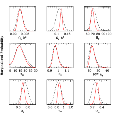
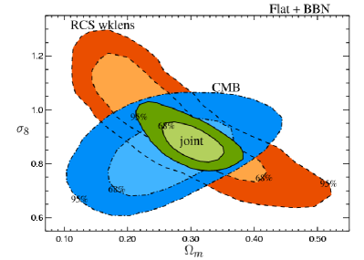
Figure 3.: left panel: one dimensional marginalized probability distribution for a selection of parameters, assuming a flat geometry of the universe from Contaldi et al. (2003). The dashed curves correspond to the CMB only results, whereas the solid curves are for the combination of CMB and RCS measurements. This demonstrates the excellent agreement between the CMB and lensing measurements, and allows us to improve the constraints on some parameters considerably. right panel: Joint likelihoods for $\Omega_{m}$ and $\sigma_{8}$. This figure clearly shows the usefulness of combining CMB and weak lensing measurements, as they are (almost) orthogonal.

Degeneracies between parameters also exist for CMB measurements, such as the results obtained from WMAP (Bennet et al. 2003; Spergel et al. 2003; Verde et al. 2003). The uncertainties in some parameters can be reduced significantly by combining the CMB results with measurements of the matter power spectrum. To this end, Verde et al. (2003) used measurements from the 2dF Field Galaxy Redshift Survey (e.g, Colless et al. 2001) and the power spectrum inferred from the Ly-$\alpha$ forest (Croft et al. 2002). The uncertainty in the bias parameter, however, limits the accuracy of the latter approach.

The weak lensing measurements can be of great use, as was shown in Contaldi et al. (2003): the combination of current cosmic shear surveys with WMAP results provides constraints on cosmological parameters that are comparable (or even better) than the largest redshift surveys. Some of the results from Contaldi et al. (2003) are shown in Figure 3. There is excellent agreement between the lensing measurements and the CMB data. Furthermore, the constraints in the $\Omega_{m}-\sigma_{8}$ plane are (almost) orthogonal.

The constraints from redshift surveys are not expected to improve dramatically in the coming years (the constraints from SDSS will tighten constraints compared to 2dF). Constraints from cosmic shear surveys, on the other hand, will improve dramatically. The signal-to-noise ratio of the improved VIRMOS-DESCART measurements is already much better than the RCS results shown here. In the next five years, the CFHT Legacy Survey (see §5) will survey an area 10 times that of the VIRMOS-DESCART survey. These developments, in conjunction with the improvement in CMB measurements, as well as other probes, make cosmic shear an important tool in “precision cosmology”.

4. Galaxy biasing

An alternative way to derive constraints on the matter power spectrum is to use the distribution of observable galaxies to infer the underlying matter distribution, under the assumption that light traces matter. On large scales the latter is likely to be true, but the drawback of galaxy redshift surveys is that the galaxies are biased tracers: the amplitude of the galaxy power spectrum is $b^{2}$ times the matter power spectrum (i.e., linear biasing), where $b$ is the bias parameter. On small scales (less than a few Mpc) the situation becomes even more unclear. Galaxy formation is a complex process, with many (unknown) feedback processes regulating the formation of stars. On these scales the galaxy bias can be non-linear, scale dependent or stochastic. This poses a problem for the interpretation of the results from galaxy redshift surveys, but can provide important observational clues for our understanding of galaxy formation.

Previously, observational constraints on the bias parameter $b$ came from measurements of the galaxy two-point correlation function, which is compared to the matter correlation function computed from numerical simulations. Such studies suggest that $b$ varies with scale, but the results rely on the assumptions made for the numerical simulations. Furthermore, this procedure cannot be used to examine how tight the correlation between the light and the matter is. To do so, we need to measure the galaxy-mass cross-correlation coefficient $r$, which is a measure of the amount of stochastic and non-linear biasing (e.g., Pen 1998; Dekel & Lahav 1999).

Weak lensing provides the most direct way to measure the galaxy-mass correlation function (e.g., Fischer et al. 2000; McKay et al. 2001; Hoekstra et al. 2003). To study the galaxy biasing we use a combination of the galaxy and mass auto-correlation functions, as well as the cross-correlation function. The bias parameters are defined in terms of the observed correlation functions through (Hoekstra et al. 2002c)

$$b^{2}=f_{1}(\theta_{\rm ap},\Omega_{m},\Omega_{\Lambda})\times\frac{\langle{N}^{2}(\theta_{\rm ap})\rangle}{\langle M_{\rm ap}^{2}(\theta_{\rm ap})\rangle},$$ (6)

and

$$r=f_{2}(\theta_{\rm ap},\Omega_{m},\Omega_{\Lambda})\times\frac{\langle M_{\rm ap}(\theta_{\rm ap}){N}(\theta_{\rm ap})\rangle}{\sqrt{\langle{N}^{2}(\theta_{\rm ap})\rangle\langle M_{\rm ap}^{2}(\theta_{\rm ap})\rangle}},$$ (7)

where $M_{\rm ap}(\theta_{\rm ap})$ is the aperture mass obtained from lensing (see Eqn. 2), and $N(\theta_{\rm ap})$ corresponds to the aperture galaxy counts (filtered with the compensated filter; see Hoekstra et al. 2002c for details). The functions $f_{1}$ and $f_{2}$ depend on the assumed cosmological model and the redshift distributions of the lenses and the sources (for details see Hoekstra et al. 2002c). The values of $f_{1}$ and $f_{2}$, however, depend minimally on the assumed power spectrum and the angular scale. There is no reason for $b$ or $r$ to be constant with scale, but as has been shown in Hoekstra et al. (2002c) we can actually measure the bias parameters as a function of scale using Eqs. 6 and 7.

Figure 4.: (a) The measured value of the galaxy-mass cross-correlation coefficient $r$ as a function of the scale for a $\Lambda$CDM $(\Omega_{m}=0.3;\Omega_{\Lambda}=0.7)$ cosmology. (b) The bias parameter $b$ as a function fo scale. The upper axis indicates the effective physical scale probed by the compensated filter at the median redshift of the lenses $(z=0.35)$. The error bars correspond to the 68% confidence intervals. Note that the measurements at different scales are slightly correlated.

Hoekstra et al. (2002c) studied the bias properties of galaxies with $19.5<R_{C}<21$. They combined the weak lensing measurements from the RCS and the VIRMOS-DESCART survey (e.g., van Waerbeke et al 2002) to obtain the first direct measurements of the bias parameter $b$ and the galaxy-mass cross-correlation coefficient $r$ as a function of scale (with scales ranging from 0.1 to 4 $h^{-1}$ Mpc). As discussed above, the VIRMOS-DESCART signal suffered from residual systematics, and Figure 4 shows the bias parameters as a function of scale, using the improved cosmic shear signal. The reduced $B$-mode on large scales significantly reduced the uncertainties in the bias parameters. In addition the variation with scale (around $\sim 5$ arcmin.) is less pronounced.

Multi-color data for the RCS have been obtained and the first catalogs have been created. The first results suggest that reliable photometric redshifts can be derived. Consequently one can start to examine the bias parameters as a function of color and luminosity, which also simplifies the comparison with predictions from models of galaxy formation.

5. Prospects

Since the first detections of lensing by large scale structure, only a few years ago, this field in observational cosmology has advanced significantly: detections have become measurements! The combination of cosmic shear measurements with CMB data already give some of the best constraints on cosmological parameters. It appears that, at least for now, most of the systematic errors are under control.

Despite these exciting recent developments, it is clear that the next generation of cosmic shear surveys requires improvements in various areas in order to be a successful tool in this era of “precision cosmology”. The Canada-France-Hawaii-Telescope Legacy Survey (CFHTLS) covers an area 10 times that of the VIRMOS-DESCART data set. Somewhat smaller surveys will be done by other telescopes (e.g., Deep Lens Survey, Subaru). This will result in a significant reduction in the statistical uncertainties. However, it is not clear that the current techniques to correct for the PSF are sufficiently accurate, but it seems plausible that the correction for the PSF can be dealt with. More problematic is the issue of the source redshift distribution. To date, redshift surveys have targeted only small areas of the sky. Some new surveys aim to cover larger areas, but the timescales for those are probably larger than the progress expected in weak lensing. Fortunately, the new lensing surveys will have photometric redshift information, which will reduce the uncertainty in the redshift distribution.

Given the above, it seems reasonable to assume that systematics can be reduced to the required level on the observational side. On the theoretical side improvements are required as well: much of the sensitivity to cosmological parameters comes from the measurements on the non-linear power spectrum. However, the current accuracy with which the latter is known is comparable to the statistical uncertainties of the VIRMOS-DESCART survey. A proper interpretation of the CFHTLS measurements will require a prediction for the non-linear power spectrum with an accuracy $\sim 1\%$ or better.

Although the analysis of the next generation of cosmic shear surveys will be a challenging task, much more ambitious projects have been proposed already. For instance the Large aperture Synoptic Survey Telescope (LSST; Tyson et al. 2002) or Panoramic Survey Telescope and Rapid Response System (Pan-STARRS; Kaiser et al. 2000) will produce massive data sets from the ground. Space based observations minimize the obervational systematics, and a weak lensing survey using the proposed SuperNova Acceleration Probe (SNAP) can provide some of the most accurate constraints on the equation of state of the universe.

To summarize these proceedings in a single sentence: the prospects for weak lensing are excellent!

References

Bacon, D., Refregier, A., & Ellis, R.S. 2000, MNRAS, 318, 625

Bacon, D., Massey, R., Refregier, A., & Ellis, R. 2003, MNRAS, 344, 673

Bartelmann, M. & Schneider, P. 2001, PhR, 340, 291

Bennet, C.L. et al. 2003, ApJS, 148, 1

Bernardeau, F., Mellier, Y., & van Waerbeke, L. 2002, A&A, 389, L28

Bernstein, G.M. & Jarvis, M. 2002, AJ, 123, 583

Brown, M.L., Taylor, A.N., Bacon, D.J., Gray, M.E., Dye, S., Meisenheimer, K., & Wolf, C. 2003, MNRAS, 341, 100

Colless, M. et al. 2001, MNRAS, 328, 1039

Contaldi, C.R., Hoekstra, H. & Lewis, A. 2003, PRL, 90, 1303

Crittenden, R.G., Natarajan, P., Pen, U.-L., & Theuns, T. 2002, ApJ, 568, 20

Croft, R.A.C., Weinberg, D.H., Bolte, M., Burles, S., Hernquist,L., Katz, N., Kirkman, D. & Tytler, D. 2002, ApJ, 581, 20

Dekel, A. & Lahav, O. 1999, ApJ, 520, 24

Fischer, P., et al. 2000, AJ, 120, 1198

Hamana, T. et al. 2002, ApJ, submitted, astro-ph/0210450

Hoekstra, H., Yee, H.K.C., Gladders, M.D., Barrientos, L.F., Hall, P.B., & Infante, L. 2002a, ApJ, 572, 55

Hoekstra, H., Yee, H.K.C., & Gladders, M.D. 2002b, ApJ, 577, 604

Hoekstra, H., van Waerbeke, L., Gladders, M.D., Mellier, Y., & Yee, H.K.C. 2002c, ApJ, 577, 595

Hoekstra, H. 2004, MNRAS, in press, astro-ph/0306097

Hoekstra, H., Yee, H.K.C., & Gladders, M.D. 2004, ApJ, submitted, astro-ph/0306515

Jain, B., & Seljak, U. 1997, ApJ, 484, 560

Jarvis, M., Bernstein, G.M., Jain, B., Fisher, P., Smith, D., Tyson, J.A., & Wittman D.M. 2003, AJ, 125, 1014

Kaiser, N., Squires, G., & Broadhurst, T. 1995, ApJ, 449, 460

Kaiser, N. 2000, ApJ, 537, 555

Kaiser, N., Tonry, J.L., Luppino, G.A. 2000, PASP, 112, 768

Kaiser, N., Wilson, G., & Luppino, G.A. 2000, ApJL, submitted, astro-ph/0003338

Kuijken, K. 1999, A&A, 352, 355

Luppino, G.A., & Kaiser, N. 1997, ApJ, 475, 20

Maoli, R., Van Waerbeke, L., Mellier, Y., Schneider, P. Jain, B., Bernardeau, F., Erben, T. & Fort, B. 2001, A&A, 368, 766

McKay, T.A., et al. 2001, ApJ, submitted, astro-ph/0108013

Peacock, J.A. et al. 2001, Nature, 410, 169

Pen, U.-L. 1998, ApJ, 504, 601

Pen, U.-L., Zhang, T., van Waerbeke, L., Mellier, Y., Zhang, P., & Dubinski, J. 2003, ApJ, 592, 664

Refregier, A., Rhodes, J., & Groth, E.J. 2002, ApJ, 572, L131

Refregier, A. & Bacon, D. 2003, MNRAS, 338, 48

Rhodes, J., Refregier, A., & Groth, E.J. 2001, ApJ, 552, L85

Schneider, P., van Waerbeke, L., Jain, B., & Kruse, G. 1998, MNRAS, 296, 873

Smith et al. 2003, MNRAS, 341, 1311

Spergel, D.N. 2003, ApJS, 148, 175

Tyson, J.A. et al. 2002, Proc. SPIE Int. Soc. Opt. Eng. 4836, 10

van Waerbeke, L., et al. 2000, A&A, 358, 30

van Waerbeke, L., et al. 2001, A& A, 374, 757

van Waerbeke, L., Mellier, Y., Pello, R., Pen, U.-L., McCracken, H.J., Jain, B. 2002, A&A, 393, 369

Verde, L. et al. 2003, ApJS,148,195

Wittman, D.M., Tyson, J.A., Kirkman, D., Dell’Antonio, I., & Bernstein, G. 2000, Nature, 405, 143