The stellar velocity distribution in the solar neighbourhood

Abstract

We explore the heating of the velocity distribution in the solar neighbourhood by stochastic spiral waves. Our investigation is based on direct numerical integration of initially circular test-particle orbits in the sheared sheet. We confirm the conclusion of other investigators that heating by spiral structure can explain the principal features of the age-velocity dispersion relation and other parameters of the velocity distribution in the solar neighbourhood. In addition, we find that heating by strong transient spirals can naturally explain the presence of small-scale structure in the velocity distribution (“moving groups”). Heating by spiral structure also explains why the stars in a single velocity-space moving group have a wide range of ages, a result which is difficult to understand in the traditional model that these structures result from inhomogeneous star formation. Thus we suggest that old moving groups arise from irregularities in the Galactic potential rather than irregularities in the star-formation rate.

1 Introduction

The velocity distribution function (df) of stars in the solar neighbourhood provides unique insights into the Galactic potential field, the dynamical history of the Galactic disk, and the relationships between kinematics, age, and metallicity for disk stars.

Let us define the Local Standard of Rest (LSR) to be a fictitious point that coincides with the Sun at the present instant and travels in a circular orbit around the Galactic centre. We introduce a rotating Cartesian coordinate system with origin at the LSR, $x$-axis pointing radially outward, $y$-axis pointing in the direction of Galactic rotation, and $z$-axis pointing to the south Galactic pole. The df $f({\bf v})$ is defined so that $f({\bf v})d{\bf v}$ is the number of stars per unit volume with velocities in the range $[{\bf v},{\bf v}+d{\bf v}]$. The standard empirical model for the past century has been the Schwarzschild (1907) df, which is a triaxial Gaussian of the form

$$f({\bf v})\propto\exp\bigg{[}-{\textstyle{1\over 2}}\sum_{i,j=1}^{3}\alpha_{ij}(v_{i}-\overline{v}_{i})(v_{j}-\overline{v}_{j})\bigg{]},$$ (1)

where ${\bf v}\equiv(v_{x},v_{y},v_{z})$. The two lowest moments of the df are the mean velocity, $\overline{\bf v}=(\overline{v}_{x},\overline{v}_{y},\overline{v}_{z})$, and the velocity-dispersion tensor,

$$\sigma^{2}_{ij}\equiv\overline{(v_{i}-\overline{v}_{i})(v_{j}-\overline{v}_{j})};$$ (2)

where $\overline{X}\equiv\int f({\bf v})X({\bf v})d{\bf v}/\int f({\bf v})d{\bf v}$, and the matrix $\sigma^{2}_{ij}$ is the inverse of the matrix $\alpha_{ij}$.

In a steady-state, axisymmetric galaxy (i) the mean velocity relative to the LSR is tangential, so $\overline{v}_{x}=\overline{v}_{z}=0$; (ii) the tensors $\alpha_{ij}$ and $\sigma_{ij}^{2}$ are both diagonal; (iii) the ratio $\sigma_{xx}^{2}/\sigma^{2}_{yy}$ is determined by the local gravitational force and its radial gradient (e.g. Chandrasekhar 1942, Binney & Tremaine 1987; see also eq. 14 below).

The velocity dispersion of stars in the solar neighbourhood increases with age, probably because the disk is “heated” by one or more dynamical mechanisms. However, the interpretation of the observed age-velocity dispersion relation (avr) is uncertain: (i) One school models the avr as a smooth power law, $\sigma_{xx}(t)\propto t^{p}$, and interprets this behavior as evidence for a continuous heating mechanism. Estimates of the exponent $p$ in the literature span the range 0.2–0.5. (ii) Some authors argue that the dispersion rises steeply with age for stars $\la 5{\rm\,Gyr}$ old, and thereafter is relatively flat (Carlberg et al., 1985; Gómez et al., 1997), perhaps because the continuous heating mechanism saturates once the dispersion is large enough. (iii) A third model is that the dispersion does not increase smoothly with age. For example, Freeman (1991) and Quillen & Garnett (2001) argue that there are three discrete age groups ($t\la 3{\rm\,Gyr}$, $3{\rm\,Gyr}\la t\la 10{\rm\,Gyr}$, $t\ga 10{\rm\,Gyr}$) with different dispersions, but within each group there is no evidence for a correlation between dispersion and age. Such groups might arise because the continuous heating saturates after only 3 Gyr, and the higher dispersion of the oldest stars is due to a discrete event such as a merger.

A wide variety of mechanisms for disk heating has been discussed (see Lacey 1991 for a review): (i) Spitzer & Schwarzschild (1951, 1953) suggested that massive gas clouds could gravitationally scatter stars, leading to a steady increase in velocity dispersion with age, and thereby predicted the existence of giant molecular clouds (gmcs). However, heating by gmcs alone fails to explain several observations (Lacey, 1984; Villumsen, 1985; Jenkins & Binney, 1990; Lacey, 1991; Jenkins, 1992): the predicted ratio $\sigma_{zz}/\sigma_{xx}$ of vertical to radial dispersion may be too high, roughly 0.72 compared to the observed value of 0.5 for old stars (but see Ida, Kokubo & Makino 1993 for an opposing view); the predicted exponent in the avr is somewhat too low, $p\la 0.25$; and the masses and number density of gmcs determined from CO observations are too low to explain the observed dispersion, probably by a factor of five or so but with substantial uncertainty. (ii) Transient spiral waves lead to potential fluctuations in the disk that excite the random motions of disk stars (Barbanis & Woltjer, 1967; Sellwood & Carlberg, 1984; Carlberg & Sellwood, 1985). However, spiral waves only excite the horizontal ($x$ and $y$) velocity components effectively, since their characteristic spatial and temporal scales are much larger than the amplitude or period of vertical oscillations for young stellar populations. (iii) These considerations lead naturally to a hybrid model, in which spiral waves excite non-circular velocities in the plane, and the velocities are then redistributed between horizontal and vertical motion through gmc scattering (Carlberg, 1987). The hybrid model has been investigated thoroughly by Jenkins & Binney (1990) and Jenkins (1992) using the Fokker-Planck equation. They find that they can successfully reproduce the observed axis ratio $\sigma_{zz}/\sigma_{xx}$, the exponent $p$ in the avr and the radial dispersion of old stars. (iv) Other possible heating mechanisms, all of which rely to some extent on hypothetical or poorly understood components or features of the Galaxy, include scattering by massive compact halo objects or halo substructure (Lacey & Ostriker, 1985), mergers with dwarf galaxies (Tóth & Ostriker, 1992; Walker, Mihos & Hernquist, 1996; Huang & Carlberg, 1997), or the outer Lindblad resonance from the Galactic bar (Kalnajs, 1991; Dehnen, 1999, 2000; Fux, 2001; Quillen, 2003).

The Schwarzschild df (1) only approximates the velocity distribution on the largest scales in velocity space. On smaller scales, there is substructure, which is most prominent in the youngest stars but present in stars of all ages. Discussion of substructure in the velocity df dates back to Kapteyn’s (1905) model of “two star streams”, and for decades Eggen advocated the case for substructure in the form of “moving groups” in the solar neighbourhood (Eggen 1996 and references therein).

Eggen and others have usually explained moving groups as the result of inhomogeneous star formation in the disk: in this model, stars in a moving group are born at a common place and time, and then disperse into a stream that happens to intersect the solar neighbourhood. This model predicts that stars in a moving group should have the same age, metallicity, and azimuthal velocity (i.e. the same angular momentum, since this determines their mean angular velocity). The existence and membership of these groups was controversial until the Hipparcos satellite measured reliable distances and proper motions for a large, homogeneous database of nearby stars, and verified the presence of rich substructure in the velocity df of both young and old stars, including a number of features that coincide with moving groups already identified by Eggen (e.g. Dehnen 1998, Chereul et al. 1998,1999)

In this paper we explore a quite different explanation for substructure in the velocity df. We suggest that substructure arises naturally from the same spiral gravitational fluctuations that excite the growth of the velocity dispersion. In other words, substructure is caused by homogeneous star formation in an irregular potential, as opposed to inhomogeneous star formation in a regular potential in the traditional model.

We investigate this hypothesis by simulating the evolution of the velocity df induced by transient spiral structure in a simple two-dimensional model of the local Galaxy. We restrict ourselves to two dimensions because spiral structure does not excite vertical motions efficiently, and because the velocity df appears to be well-mixed in the vertical direction (Dehnen, 1998).

Following Eggen, we shall use the term “moving group” to denote substructure in the velocity df of old stars ($\ga 1$ Gyr) at a given position. Unfortunately, the same term is sometimes also applied to OB associations, which are spatially localized concentrations of much younger stars (e.g., de Zeeuw et al. 1999).

Section 3 describes our simplified dynamical model. The results of our simulations are analyzed and compared to observed data in §4. Section 5 examines briefly the traditional hypothesis that substructure arises from inhomogeneous star formation. Section 6 contains a brief discussion of the closely related process of radial migration of stars, and §7 contains concluding remarks.

2 Properties of spiral structure

Our model depends on several properties of the Galaxy’s spiral structure, such as the number of arms, the arm strength, and the pitch angle. We are concerned with spiral structure in the disk surface density (rather than, say, in the distribution of young stars or gas). The properties of this structure in external galaxies are revealed by near-infrared images, which are dominated by the stars that contribute most of the mass (Rix & Rieke 1993, but see also Rhoads 1998 and James & Seigar 1999 for qualifications).

Rix & Zaritsky (1995) examined the K-band spiral structure of 18 face-on galaxies. They found that almost half had strong two-arm ($m=2$) spirals, with arm-interarm contrasts $I_{\rm max}/I_{\rm min}\simeq 2$. If the arms are sinusoidal, with fractional amplitude $\epsilon$ relative to the axisymmetric background, the arm-interarm contrast is $I_{\rm max}/I_{\rm min}=(1+\epsilon)/(1-\epsilon)$, so a contrast of 2 corresponds to $\epsilon\simeq 0.3$.

Block & Puerari (1999) examined K-band spiral structure in 19 spirals. They found pitch angles ranging from $8\degr$ to $49\degr$ with a median value of $22\degr$, and $m=2$ amplitudes ranging from $\epsilon=0.03$ to $\epsilon=0.5$, with a median $\epsilon=0.1$.

Seigar & James (1998) conducted a similar survey of 45 galaxies. They found that the dominant Fourier mode usually has $m=1$ (36%) or $m=2$ (31%), and the median pitch angle of the spiral structure was $8\degr$, with little or no correlation with Hubble type. They measure the strength of the spiral arms in terms of the “equivalent angle”; their median equivalent angle of $14\degr$ corresponds to an amplitude $\epsilon\simeq 0.07$ for a sinusoidal $m=2$ spiral.

Elmegreen et al. (1999) stress that the amplitude of $m=2$ spiral structure in the near-infrared depends on whether the optical spiral arms are classified as flocculent or grand-design (Elmegreen, 1998). Grand-design spirals have arm-interarm contrasts of 1.5–6, corresponding to amplitude $\epsilon=0.2$–0.7, while flocculent galaxies have contrast $\la 1.7$, corresponding to $\epsilon\la 0.25$.

At optical wavebands, Ma et al. (1999) find that the mean pitch angle for 51 Sbc galaxies (the same Hubble type as the Galaxy) is $15\degr$.

The measurement of spiral structure in our own Galaxy is more difficult than in face-on external galaxies. Drimmel (2000) uses K-band photometry of the Galactic plane to conclude that the Galaxy contains a two-arm spiral with pitch angle $18\degr$. Vallée (2002) reviews a number of studies of the Galaxy’s spiral structure, mostly based on young stars, gas and dust; these yield a range of pitch angles from $6\degr$–$20\degr$, but Vallée concludes that the best overall fit is provided by an $m=4$ spiral with pitch angle of $12\degr$. The arm structure in the Galaxy appears to be intermediate between grand-design and flocculent (Elmegreen, 1998).

3 A numerical model of disk heating

We model disk heating in the sheared sheet, which approximates the local dynamics of a differentially rotating disk (Spitzer & Schwarzschild, 1953; Goldreich & Lynden-Bell, 1965; Julian & Toomre, 1966). The LSR is assumed to travel around the Galactic centre in a circular orbit of radius $R_{0}$ and angular frequency $\Omega>0$. We use the same Cartesian coordinate system $(x,y,z)$ introduced in the last Section, restrict ourselves to the $z=0$ plane, and denote position and velocity by ${\bf x}=(x,y)$ and ${\bf v}=(\dot{x},\dot{y})$. For $|x|,|y|\ll R_{0}$ the equations of motion of a test particle are

$$\ddot{x}-2\Omega\dot{y}-4\Omega Ax = -\frac{\partial\Phi}{\partial x},$$

$$\ddot{y}+2\Omega\dot{x} = -\frac{\partial\Phi}{\partial y},$$ (3)

where $\Phi({\bf x},t)$ is the gravitational potential due to sources other than the axisymmetric Galactic disk, and $A>0$ is the Oort constant

$$A=-\frac{1}{2}\left(R\frac{d\Omega}{dR}\right)_{R_{0}},$$ (4)

where $R\Omega(R)$ is the circular speed at radius $R$ and $\Omega(R_{0})=\Omega$.

If $\Phi$ = 0 the trajectories governed by equations (3) have two integrals of motion related to energy and angular momentum,

$$E\equiv{\textstyle{1\over 2}}(\dot{x}^{2}+\dot{y}^{2}-4\Omega Ax^{2}),\qquad H\equiv\dot{y}+2\Omega x.$$ (5)

The solutions of the equations of motion are

$$x = x_{g}+a\cos(\kappa t+\phi),$$

$$y = y_{g}(t)-\frac{2\Omega}{\kappa}a\sin(\kappa t+\phi),$$

$$y_{g}(t) = y_{g0}-2Ax_{g}t,$$ (6)

where $[x_{g},y_{g}(t)]$ are the coordinates of the guiding centre, $a$ is the epicycle amplitude, $\phi$ is a phase constant, and $\kappa$ is the radial or epicycle frequency,

$$\kappa=\Omega\left(4+2\frac{d\ln\Omega}{d\ln R}\right)^{1/2}_{R_{0}}\quad\hbox{or}\quad\kappa^{2}=4\Omega(\Omega-A).$$ (7)

The energy and angular momentum are related to the guiding-centre radius and epicycle amplitude by

$$E=2A(A-\Omega)x_{g}^{2}+{\textstyle{1\over 2}}\kappa^{2}a^{2},\qquad H=2(\Omega-A)x_{g},$$ (8)

and the guiding-centre radius is related to the phase-space coordinates by

$$x_{g}={\dot{y}+2\Omega x\over 2(\Omega-A)}.$$ (9)

The epicycle energy is defined as

$$E_{x} \equiv {\textstyle{1\over 2}}\left[\dot{x}^{2}+\kappa^{2}(x-x_{g})^{2}\right]$$ (10)

$$= E+{AH^{2}\over 2(\Omega-A)}$$

$$= {\textstyle{1\over 2}}\kappa^{2}a^{2}$$

$$= {\textstyle{1\over 2}}\dot{x}^{2}+{2\Omega^{2}\over\kappa^{2}}(\dot{y}+2Ax)^{2}.$$

The epicycle energy is closely related to the radial action

$$I={\textstyle{1\over 2}}\kappa a^{2}=E_{x}/\kappa.$$ (11)

For a particle in a circular orbit,

$$(x,y,\dot{x},\dot{y})=(x_{g},y_{g0}-2Ax_{g}t,0,-2Ax_{g}),$$ (12)

thus ${E_{x}=0}$.

The approximations used in deriving the linearized equations of motion (3) are only marginally valid in the solar neighbourhood, since the epicycle amplitudes $a$ can be a significant fraction of $R_{0}$ (for a population with radial velocity dispersion $\sigma_{xx}$ in a galaxy with a flat rotation curve,

$$\overline{a^{2}}=\sigma_{xx}^{2}/\Omega^{2}.$$ (13)

Thus old disk stars in the solar neighbourhood, with $\sigma_{xx}\simeq 40{\rm\,km\,s^{-1}}$, have $(\overline{a^{2}})^{1/2}\simeq 0.18R_{0}$). Nevertheless, we believe that the sheared sheet accurately captures the most important features of the evolution of disk-star kinematics.

The kinematics of a population of stars is described by the df $f({\bf x},{\bf v},t)$, where $fd{\bf x}d{\bf v}$ is the number of stars in the interval $({\bf x},{\bf v})\to({\bf x}+d{\bf x},{\bf v}+d{\bf v})$. According to Jeans’s theorem (Binney & Tremaine, 1987), a stationary df can only depend on the integrals of motion $E$ and $H$ (or $E_{x}$, $x_{g}$, $a$, etc.). In the solar neighbourhood ($x=y=0$), the integrals are $H=\dot{y}$ and $E_{x}={\textstyle{1\over 2}}\dot{x}^{2}+2\Omega^{2}\dot{y}^{2}/\kappa^{2}$. Thus in a steady state the velocity distribution must be an even function of $\dot{x}$.

It is straightforward to show that the mean velocity and velocity-dispersion tensor of any stationary, spatially homogeneous df in the sheared sheet must satisfy the relations

$$\overline{v}_{x}=0,\ \overline{v}_{y}=-2Ax,\ \sigma^{2}_{xy}=\sigma^{2}_{yx}=0,\ {\sigma^{2}_{xx}\over\sigma^{2}_{yy}}={\Omega\over\Omega-A}.$$ (14)

A useful model df for the sheared sheet is

$$f({\bf x},{\bf v})\propto\exp\left(-E_{x}/\sigma_{0}^{2}\right),$$ (15)

where $E_{x}$ is defined in equation (10). At a given location, the df (15) leads to a two-dimensional version of the triaxial Gaussian velocity distribution (1), in which the mean velocity and velocity-dispersion tensor satisfy the relations (14). Thus the df (15) is also sometimes (confusingly) called the Schwarzschild df.

In our simulations the relations (14) are not satisfied exactly, so it is useful to introduce the principal-axis system $(x_{1},x_{2})$ in which the velocity-dispersion tensor is diagonal; the $x_{1}$-axis is chosen to lie within $45\degr$ of the $x$-axis. The corresponding velocity dispersions are $\sigma_{1}$ and $\sigma_{2}$, which we will normally plot instead of $\sigma_{xx}$ and $\sigma_{yy}$; usually in our simulations and in the data we shall find that $\sigma_{1}>\sigma_{2}$. The vertex deviation $l_{v}$ is the Galactic longitude of the $x_{1}$-axis, and is given by

$$l_{v}\equiv-\frac{1}{2}\arctan{\left(\frac{2\sigma^{2}_{xy}}{\sigma^{2}_{xx}-\sigma^{2}_{yy}}\right)},$$ (16)

where $|l_{v}|<45\degr$. Stellar populations in the solar neighbourhood have vertex deviations in the range $0\la l_{v}\la 30\degr$ (Binney & Merrifield, 1998).

Throughout the paper, we assume that the rotational curve of the underlying axisymmetric galaxy is flat, $R\Omega(R)=\hbox{constant}$, so that $A={1\over 2}\Omega$ and $\kappa=\sqrt{2}\Omega$. We shall assume that the surface density of the disk in the solar neighbourhood is $\Sigma_{d}=50M_{\odot}{\rm\,pc}^{-2}$; recent observational estimates are $\Sigma_{d}=40M_{\odot}{\rm\,pc}^{-2}$ (Crézé et al., 1998), $48M_{\odot}{\rm\,pc}^{-2}$ (Holmberg & Flynn, 2000), and $42\pm 6M_{\odot}{\rm\,pc}^{-2}$ (Korchagin et al., 2003). The assumed surface density only enters our analysis through the definition of the fractional spiral amplitude $\epsilon$ below (eq. 21).

3.1 Spiral waves

We approximate spiral structure as a superposition of waves with surface density and potential

$$\Sigma(x,y,t) = \Sigma_{s}(t)\,\exp i(k_{x}x+k_{y}y),$$

$$\Phi(x,y,t) = \Phi_{s}(t)\,\exp i(k_{x}x+k_{y}y),$$ (17)

where ${\bf k}=(k_{x},k_{y})$ is the wavenumber, and only the real part of $\Sigma$ or $\Phi$ is physical. Without loss of generality we can assume that $k_{y}\geq 0$; then the spiral is trailing if $k_{x}>0$ and leading if $k_{x}<0$. In this paper, we only consider trailing spiral waves. The number of arms $m$ and the pitch angle $\alpha$ are determined by ${\bf k}$ through the relations

$$k_{y}=\frac{m}{R_{0}},\hskip 36.135pt\left|\frac{k_{y}}{k_{x}}\right|=\tan\alpha.$$ (18)

The relation between potential and surface density for spiral waves is given by (e.g. Binney & Tremaine 1987)

$$\Phi_{s}(t)=-\frac{2\pi G\Sigma_{s}(t)}{k},$$ (19)

where $k=|{\bf k}|$.

Steady spirals, in which $\Sigma_{s}(t),\Phi_{s}(t)\propto\exp(i\omega t)$, heat stars on nearly circular orbits only at the Lindblad resonances (Lynden-Bell & Kalnajs, 1972), which occur at the guiding centre radii given by

$$\omega=2Ak_{y}x_{g}\pm\kappa.$$ (20)

We focus instead on transient spiral structure, which can heat stars over a range of radii. We model each transient spiral using a Gaussian amplitude dependence centred at time $t_{s}$ with standard deviation $\sigma_{s}$:

$$\Phi_{s}(t)={2\pi\epsilon G\Sigma_{d}\over k}\exp\left[-\frac{(t-t_{s})^{2}}{2\sigma_{s}^{2}}+i(\theta+2Ak_{y}x_{c}t)\right].$$ (21)

Here $\theta$ is a phase constant, and $x_{c}$ is the corotation radius relative to the LSR (the phase of the spiral is constant for an observer on a circular orbit at $x_{c}$). The parameter $\epsilon$ measures the amplitude of the spiral, and the normalizing constants are chosen so that the maximum surface density in the spiral is a fraction $\epsilon$ of the surface density of the underlying disk (eq. 19).

In each simulation the trajectories of the stars were followed between time $t=0$ and $t=t_{0}$. During this interval the stars were perturbed by $N_{s}$ transient spiral waves. Each wave had phase constant $\theta$ chosen randomly from $[0,2\pi]$, corotation radius $x_{c}$ chosen randomly from a Gaussian distribution centred on the LSR with standard deviation $\sigma_{c}$, and central time $t_{s}$ chosen randomly from $[-2\sigma_{s},t_{0}+2\sigma_{s}]$ (this is slightly longer than the integration interval, to include the effects of transients whose wings are inside the integration interval although their central times are not).

The fractional amplitude of the surface-density perturbation due to a single transient spiral is $\epsilon$ at the wave peak. However, in some ways a better quantity to compare with the observational data on spiral amplitudes is the root-mean-square (rms) time average of the fractional surface-density amplitude,

$$\epsilon_{{\caps rms}}=\epsilon\left(\pi^{1/2}N_{s}\sigma_{s}\over t_{0}\right)^{1/2}.$$ (22)

A closely related quantity is the rms potential perturbation,

$$\Phi_{{\caps rms}}=2\pi G\epsilon_{{\caps rms}}\Sigma_{d}R_{0}{|\sin\alpha|\over\sqrt{2}m};$$ (23)

(the factor $\sqrt{2}$ arises because $\Phi_{{\caps rms}}$ is the rms fluctuation rather than the rms amplitude, which is smaller by $\sqrt{2}$). Jenkins & Binney (1990) use Fokker-Planck calculations of heating by transient spiral structure to estimate that $\Phi_{{\caps rms}}=(9\hbox{--}13{\rm\,km\,s^{-1}})^{2}$.

The power spectrum of each transient is a Gaussian with standard deviation $(2\sigma_{s}^{2})^{-1/2}$. The central frequencies of the power spectra of the transients follow a Gaussian distribution with standard deviation $2Ak_{y}\sigma_{c}$. Thus the power spectrum of the ensemble of $N_{s}$ transients is smooth if the overlap factor

$$C\equiv N_{s}{(2\sigma_{s}^{2})^{-1/2}\over 2Ak_{y}\sigma_{c}}={N_{s}\over 2^{3/2}Ak_{y}\sigma_{c}\sigma_{s}}$$ (24)

is large compared to unity; on the other hand if $C\ll 1$ the power spectrum and hence the heating is localized at narrow resonances. All of our simulations have $C\gg 1$ (see Table 1).

The dispersion of the power spectrum of all the transients is $\sigma_{t}$, given by

$$\sigma_{t}^{2}={1\over 2\sigma_{s}^{2}}+(2Ak_{y}\sigma_{c})^{2}.$$ (25)

Note that in this model problem different azimuthal wavenumbers $m$ and $m^{\prime}=fm$ are equivalent if we rescale the other variables by: ${\bf k}^{\prime}=f{\bf k}$, $\alpha^{\prime}=\alpha$, $t^{\prime}=t$, $(x^{\prime},y^{\prime})=(x/f,y/f)$, $\Phi_{s}^{\prime}=\Phi_{s}/f^{2}$, $\Sigma_{s}^{\prime}=\Sigma_{s}/f$, $\epsilon^{\prime}=\epsilon/f$, $\sigma^{\prime}_{ij}=\sigma_{ij}/f$ $\sigma_{c}^{\prime}=\sigma_{c}/f$, $\sigma_{0}^{\prime}=\sigma_{0}/f$, $\sigma_{s}^{\prime}=\sigma_{s}$.

3.2 Determining the solar neighbourhood velocity distribution

Assume that the disk stars are formed on circular orbits at time $0$. We wish to determine the velocity distribution at the present time $t_{0}$ in the solar neighbourhood, $(x,y)=(0,0)$. This is a two-point boundary-value problem rather than an initial-value problem: the boundary conditions on the phase-space coordinates are $(x,y,\dot{x},\dot{y})=(x_{g},y_{g0},0,-2Ax_{g})$ at $t=0$ (on circular orbits) and $(x,y)=(0,0)$ at $t=t_{0}$ (in the solar neighbourhood). The solutions to the boundary-value problem will be a set of distinct initial positions $[x_{i}(t=0),y_{i}(t=0)]$ or final velocities $[\dot{x}_{i}(t=t_{0}),\dot{y}_{i}(t=t_{0})]\equiv(-u_{i},v_{i})$, $i=1,2,\ldots$ (the sign of $u$ is chosen to agree with the usual convention that stars moving towards the Galactic centre have $u>0$). Because the motion of stars in the fluctuating gravitational field of the transient spirals is complicated, we expect that there will be many solutions. In this idealized model the velocity-space df in the solar neighbourhood will consist of a set of delta-functions at the velocities $(u_{i},v_{i})$, but in practice these will be smeared into a continuous distribution by observational errors, the non-zero volume of the “solar neighbourhood”, the small initial velocity dispersion of the stars when they are formed, etc.

Normally, boundary-value problems are solved most efficiently by iterative methods. In this case, however, most of the solutions have only a tiny domain of attraction in the $(u,v)$ plane; thus iterative methods are inefficient. We have therefore adopted a different approach, based on Monte Carlo sampling (Dehnen, 2000).

Stars are not born on precisely circular orbits, in part because star-forming clouds are not on circular orbits. We may therefore assume that the stars initially have a Schwarzschild df (eq. 15), with a small but non-zero initial velocity dispersion $\sigma_{0}$.

Following Dehnen, we integrate orbits backward in time, starting at $t=t_{0}$ (which we call the initial integration time or “present epoch”) and ending at $t=t_{0}$ (the final integration time or “formation epoch”). The initial conditions are chosen at random from $(x,y,\dot{x},\dot{y})=(0,0,-u,v)$, with $|u|,|v|<v_{\rm max}$. We choose $v_{\rm max}=110{\rm\,km\,s^{-1}}$, large enough to include almost all disk stars in the solar neighbourhood. We then integrate equations (3) backwards in time to the formation epoch. The collisionless Boltzmann equation (Binney & Tremaine, 1987) states that the phase-space density around a trajectory is time-invariant. Therefore the phase-space density $F_{i}$ at $(u_{i},v_{i})$ at the present epoch is given by (15), where the epicycle energy $E_{x}$ is measured at the formation epoch. We assume that the spatial volume of our survey of the solar neighbourhood is independent of velocity, so the density in velocity space at the present epoch is proportional to $F_{i}$. Dehnen’s procedure therefore provides a Monte Carlo sampling of the velocity-space df at the present epoch.

We convert our Monte Carlo realization to a smooth df by convolution with observational errors. We replace the point solutions ${\bf v}_{i}=(u_{i},v_{i})$ by Gaussians, that is,

$$f({\bf v})=\sum_{i}F_{i}\delta({\bf v}-{\bf v}_{i})$$ (26)

is replaced by

$$f({\bf v})={1\over 2\pi\sigma_{\rm ob}^{2}}\sum_{i}F_{i}\exp\left[-{({\bf v}-{\bf v}_{i})^{2}\over 2\sigma_{\rm ob}^{2}}\right],$$ (27)

where $\sigma_{\rm ob}$ is the assumed observational error.

We have described the procedure for estimating the df of stars of age $t_{0}$, using equation (15) and the epicycle energies at $t=0$. However, we can also determine the df for stars having an intermediate age $t_{0}-t_{m}$ in the course of the same orbit integration, using the epicycle energies of the stars at the intermediate time $t_{m}$. This approach measures the dependence of the df on stellar age, and thus determines the avr for a given realization of the set of transient spiral arms, using only a single set of orbit integrations.

3.3 Units and model parameters

The time unit is chosen to be $\Omega^{-1}$ and the distance unit is chosen to be $R_{0}$. The azimuthal orbital period is then $2\pi/\Omega=2\pi$. For conversion to physical units we assume that $R_{0}=8{\rm\,kpc}$ and $\Omega R_{0}=220{\rm\,km\,s^{-1}}$, so that the unit of time is 35.6 Myr. Most of our numerical integrations ran for an interval $t_{0}=281$, corresponding to 40.8 rotation periods of the LSR or 10.0 Gyr.

We consider only trailing spirals with $m=2$ or $m=4$. The standard deviation of the distribution of corotation radii for the transient spirals was $\sigma_{c}=0.25$ corresponding to 2 kpc. With these choices the overlap factor is $C=1.41N_{s}(m/2)/(\Omega\sigma_{s})$.

The radial velocity dispersion of stars at the time of their birth is taken to be $\sigma_{0}=3{\rm\,km\,s^{-1}}$. The observational error in the velocities is taken to be $\sigma_{\rm ob}=3{\rm\,km\,s^{-1}}$; for the typical Hipparcos parallax error of 1 mas, $\sigma_{\rm ob}$ corresponds to the velocity error arising from the distance uncertainty for a star with transverse velocity $30{\rm\,km\,s^{-1}}$ at a distance of 100 pc.

In each simulation we launch either $1\times 10^{7}$ or $7\times 10^{7}$ stars from the solar neighbourhood and integrate back for 10 Gyr (the smaller simulations are used to estimate moments, such as those in Figure 1, and the larger simulations are used to estimate the df, as in Figure 7). In the larger simulations, typically 10000–15000 stars contribute significantly to the solution, in the sense that their epicycle energy at the formation epoch is $<3\sigma_{0}^{2}$. This number is larger than the number of stars in the Hipparcos samples to which we compare (e.g. 4600 in the largest color-selected sample analysed by Dehnen 1998). We have verified that the conclusions below are unaffected if we double the number of stars in the simulation or change the random-number seed used to select the sample of stars (keeping the same seed to select the spiral transients).

Table 1: Simulation parameters

Parameter	Symbol	Run R5	Run R10	Run R20	Run R40	Run Rm4	Run Rsim
Defining parameters
Number of spiral arms	$m$	2	2	2	2	4	2
Number of spiral waves	$N_{s}$	45	18	12	9	12	48
Maximum fractional surface
density of spiral waves	$\epsilon$	1.61	0.80	0.80	0.67	0.80	0.31
Time scale of spiral waves	$\sigma_{s}$	1	1	1	1	1	1
rms corotation radius $(R-R_{0})/R_{0}$	$\sigma_{c}$	0.25	0.25	0.25	0.25	0.25	0.25
Pitch angle	$\alpha$	$5\degr$	$10\degr$	$20\degr$	$40\degr$	$20\degr$	$20\degr$
Derived parameters
Overlap factor (eq. 24)	$C$	64	25	17	13	34	68
rms surface-density amplitude (eq. 22)	$\epsilon_{{\caps rms}}$	0.86	0.27	0.22	0.16	0.22	0.17
rms potential in $({\rm\,km\,s^{-1}})^{2}$ (eq. 23)	$\Phi_{{\caps rms}}$	$(16.9)^{2}$	$(13.4)^{2}$	$(17.0)^{2}$	$(19.8)^{2}$	$(12.0)^{2}$	$(15.0)^{2}$

We carried out a number of simulations with different values of the spiral-wave parameters $m$ (number of arms), $N_{s}$ (number of spirals), $\epsilon$ (fractional surface-density perturbation), $\sigma_{s}$ (duration of the transient), $\sigma_{c}$ (dispersion in corotation radius), and $\alpha$ (pitch angle). The parameters of the simulations are shown in Table 1. Each simulation is defined by these six parameters and the random number seeds for both the stars and the spiral arms.

Our runs have pitch angles of $5\degr$, $10\degr$, $20\degr$, and $40\degr$, which span the range of observed pitch angles in spiral galaxies. We then choose the amplitude $\epsilon$ and the number of transients $N_{s}$ to approximately reproduce the observed radial velocity dispersion of old main-sequence stars in the solar neighbourhood.

All of our runs have two-armed spirals ($m=2$), except for run R_m4, which has the same parameters as run R₂₀ except that $m=4$.

We also have run R_sim, in which we have used a larger number of weaker transients than in run R₂₀, and have also adjusted some of the central times of the spiral transients to better reproduce the features of the observed solar neighbourhood df (see §4.4).

The rms potential fluctuation $\Phi_{{\caps rms}}=(13\hbox{--}20{\rm\,km\,s^{-1}})^{2}$ in our four runs, higher than the velue $\Phi_{{\caps rms}}=(9\hbox{--}13{\rm\,km\,s^{-1}})^{2}$ derived by Jenkins & Binney (1990) from Fokker-Planck calculations by about a factor of 2–2.4. A minor component of this difference arises because Jenkins & Binney (1990) include gmcs, which contribute about 20% of their total heating rate. A more important effect, pointed out to us by A. J. Kalnajs, is that in our model the heating is spatially inhomogeneous: our assumptions place the Sun fairly close to corotation for most of the transients, so that heating at the Lindblad resonances is more effective inside and outside the solar circle than it is at the solar circle.

The fractional surface-density fluctuation $\epsilon$ required to reproduce the avr in run R₅ exceeds unity, and the rms surface-density fluctuation is close to unity; these high values are unrealistic and suggest that a larger number of weaker transients is required if the pich angle is as small as $5\degr$.

Runs R₁₀, R₂₀, R₄₀, and R_m4 have peak amplitudes $\epsilon=0.7$–$0.8$, similar to the strongest grand-design spirals, but these large amplitudes are only present for a small fraction of the time ($N_{s}\sigma_{s}/t_{0}=0.03$–0.06). The relatively small number of high-amplitude transients in these runs is consistent with a model in which the Galaxy has experienced several short-lived grand-design spiral phases, possibly caused by minor mergers. In contrast, run R_sim has a much larger number of weaker transients ($\epsilon=0.3$, $N_{s}\sigma_{s}/t_{0}=0.17$).

Each run was repeated seven times (realizations a-g), using different random-number seeds to generate both the stars and the spiral transients, in order to distinguish systematic from stochastic variations. To study extremely long-term behavior, we also ran a realization h, in which both the integration time and the number of transients are a factor of three larger than in a-g.

Figure 1: The age dependence of the principal axes of the velocity-dispersion tensor in runs R₅, R₁₀, R₂₀ and R₄₀. The solid line shows $\sigma_{1}$ and the dashed line shows $\sigma_{2}$. The three rows (a,b,c) represent different realizations. The dot-dashed lines show the best fit of equation (29) for each realization; see also Table 3.

4 Results

Table 2: Simulation results and observations

Quantity	Symbol	Run R5	Run R10	Run R20	Run R40	Run Rm4	Run Rsim	Observations
Radial velocity dispersion	$\sigma_{xx}({\rm\,km\,s^{-1}})$	$36\pm 1$	$38\pm 2$	$40\pm 4$	$39\pm 6$	$35\pm 3$	$40\pm 3$	36.9
vertex deviation	$l_{v}(\degr)$	$-3\pm 4$	$3\pm 3$	$8\pm 16$	$-8\pm 12$	$3\pm 8$	$-6\pm 11$	10.9
axis ratio of velocity ellipsoid	$\sigma_{1}/\sigma_{2}$	$1.3\pm 0.1$	$1.4\pm 0.1$	$1.2\pm 0.1$	$1.3\pm 0.1$	$1.4\pm 0.1$	$1.4\pm 0.2$	1.48
mean radial velocity	$\overline{u}({\rm\,km\,s^{-1}})$	$0\pm 4$	$-1\pm 3$	$0\pm 5$	$3\pm 1$	$0\pm 4$	$0\pm 8$	$-0.5$
mean azimuthal velocity	$\overline{v}({\rm\,km\,s^{-1}})$	$0\pm 2$	$0\pm 2$	$-1\pm 3$	$3\pm 1$	$-2\pm 3$	$2\pm 5$	$-17.7$

Results given are the mean and standard deviation from realizations a–g, for a population of stars with ages uniformly distributed between 0 and 10 Gyr. “Observations” column gives results from samples B4+GI from Dehnen (1998), which contains stars redward of the Parenago discontinuity ($B-V>0.6$, for which the lifetime of main-sequence stars exceeds the age of the Galaxy) and giant stars. The large negative mean azimuthal velocity in the observations is due to the asymmetric drift, which is not present in our simulations.

4.1 Age-velocity dispersion relation

In §3.2, we have shown that a single set of orbit integrations can be used to derive the df for stars of all ages between 0 and $t_{0}$. Thus we may combine dfs of different ages to produce the df that corresponds to a uniform distribution of ages between 0 and 10 Gyr (hereafter the “combined df”), as would result from a uniform star-formation rate. The average moments of this df for our runs are shown in Table 2, along with the observed values taken from Dehnen (1998). Of course, the close agreement of the radial velocity dispersion $\sigma_{xx}$ in each run with the observed value of $37{\rm\,km\,s^{-1}}$ arises because the strength and number of spiral transients were chosen to produce the correct radial dispersion.

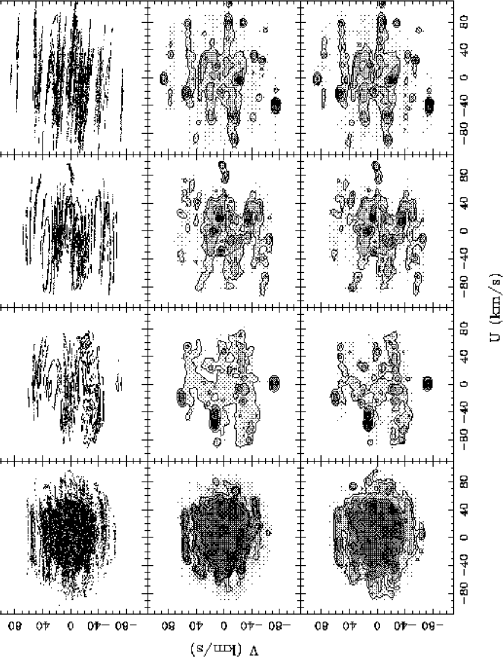
The evolution of the principal axes ${\sigma}_{1}$ and ${\sigma}_{2}$ of the velocity-dispersion tensor in runs R₅, R₁₀, R₂₀ and R₄₀ is shown in Figure 1. The three rows of panels show the results for three different realizations, i.e., three different sets of random-number seeds used to generate both the stars and the spiral transients. In general, the results in this and other figures are independent of the realization of the stellar distribution, and all of the variations seen are due to changes in the realization of the transient spiral structure—a reflection of the fact that the Monte Carlo simulation of the stellar distribution is a numerical method while the simulation of the distribution of spiral transients is a model of a stochastic physical process.

The avrs illustrate the following:

• Open spirals (large pitch angle) heat the disk stars more effectively than tightly wound spirals. For example, both the number $N_{s}$ and the surface-density amplitude $\epsilon$ of the spiral transients are larger in R₅ than the other runs shown (see Table 1), even though all runs produce the same velocity dispersion by design.

• The heating occurs in discrete steps separated by periods of zero growth. This feature arises because we have only a small number of spiral transients over the course of the simulation, each of which has the same amplitude and lasts only for a characteristic time $\sigma_{s}=1$ out of the total integration time of $281$. During the intervals between the spiral transients, the df is stationary so the velocity dispersions are constant.

• In run R₅ the growth of the dispersion slows sharply after the radial dispersion reaches $\sim 30{\rm\,km\,s^{-1}}$. This effect probably arises because the epicycle amplitude becomes comparable to the radial spacing between the spiral arms, so that the forces from the spirals tend to average to zero over an epicycle oscillation. More specifically, the radial spacing of the spiral arms is $\Delta x=2\pi R_{0}\tan\alpha/m$; the rms epicycle amplitude $(\overline{a^{2}})^{1/2}$ is given by equation (13), and we expect the spiral heating to become ineffective when the rms epicycle amplitude exceeds the peak-to-trough distance between arms, that is, when $(\overline{a^{2}})^{1/2}/\Delta x\ga 0.5$. For small pitch angle $\alpha$,

  $${(\overline{a^{2}})^{1/2}\over\Delta x}={m\sigma_{xx}\over 2\pi\Omega R_{0}\tan\alpha}\simeq 0.50{m\over 2}{\sigma_{1}\over 30{\rm\,km\,s^{-1}}}{5\degr\over\alpha}.$$ (28)

• There are substantial differences among the realizations of a given run; in other words there are significant stochastic effects in spiral-wave heating (see the discussion of the exponent $p$ below for further detail). The stochastic variations in the heating rate become smaller as the velocity dispersion increases (see also Figure 2, which follows the avrs over an even longer time interval).

For comparisons with theoretical models, it is useful to fit the simulated avrs with a parametrized function. A common parametrization (e.g. Lacey 1991) is

$$\sigma_{1}(t)=(\sigma_{0}^{1/p}+Ct)^{p},$$ (29)

where $\sigma_{0}$ is the initial dispersion along the major principal axis, fixed at $3{\rm\,km\,s^{-1}}$ as in §3.3. The motivation for this form is the assumption that the evolution of the dispersion is governed by a diffusion equation with velocity-dependent diffusion coefficient,

$$\frac{d\sigma_{1}^{2}(t)}{dt}=C_{1}\sigma_{1}^{-q}(t),$$ (30)

where $C_{1}=2pC$ and $q=p^{-1}-2$, with $C$, $p$ and $q$ constants. For ${\sigma}_{1}\gg{\sigma}_{0}$, equation (29) implies $\sigma_{1}(t)\propto t^{p}$.

The dashed lines in Figure 1 show the results of least-squares fits for the parameters $C$ and $p$ in equation (29). In each case, the fitting function successfully preserves the overall shape of the avr but smooths over fluctuations due to the finite number of transients. We fit each of the seven realizations of each run and obtained the values of the avr exponent $p$ given in Table 3. The standard deviation in $p$ can be as large as 35% (in run R₂₀) among realizations of a single parameter set, and the variation due to changes in the spiral-structure parameters is just as large. Thus, the exponent of the avr is not likely to discriminate well between heating by transient spiral structure and heating by other mechanisms.

Figure 2 shows the avrs of realization h, which was run for $t_{0}=30$ Gyr, three times as long as the other runs. The purpose of this long run was to see how well the parametrization (29) worked as the heating process continued. The dashed lines show that equation (29) still provides a reasonable fit; however, the best-fit exponent $p$ (see Table 3) is systematically smaller than in the shorter realizations a–g, except in run R₅. Therefore, equation (29) should be considered as a fitting function valid over a limited time interval, rather than a formula with predictive power.

All of our runs have the same value of the parameter $\sigma_{s}$ (Table 1), which represents the duration of the spiral transients. We have experimented with a range of values of $\sigma_{s}$. As shown in Figure 3, the dispersion for the combined df with a uniform distribution of ages between 0 and 10 Gyr is almost independent of $\sigma_{s}$ so long as $\sigma_{s}\ga 0.5$. A probable explanation is that the width of the power spectrum of the transient perturbations, given by equation (25), is dominated by the dispersion in pattern speeds rather than the duration of a single transient once $\sigma_{s}\ga 1/(2\sqrt{2}Ak_{y}\sigma_{c})$, which occurs when $\sigma_{s}\ga 1.4$ for our parameters. Of course, when $\sigma_{s}$ becomes very large, the overlap factor of equation (24), will decrease below unity and the heating will be localized at discrete resonances.

Figure 2: The evolution of the avr over 30 Gyr. The dashed lines show the best-fit models of the form (29); see also Table 3.

Figure 3: The dependence of the velocity dispersion on the duration of the transients, derived from the combined df for a population of stars with a uniform distribution of ages up to 10 Gyr. All of the runs plotted in a given panel use the same defining parameters as in Table 1, except for the transient duration ${\sigma_{s}}$. The solid and dashed lines show ${\sigma_{xx}}$ and ${\sigma_{yy}}$, respectively. The velocity dispersion is almost independent of the transient duration ${\sigma_{s}}$, except for $\sigma_{s}\la 0.5$.

Table 3: Fitted exponent $p$ of avrs (eq. 29).

	a	b	c	d	e	f	g	a–g	h
R5	0.31	0.20	0.22	0.27	0.27	0.22	0.31	0.25$\pm$0.05	0.24
R10	0.30	0.34	0.37	0.32	0.24	0.24	0.25	0.29$\pm$0.05	0.25
R20	0.33	0.46	0.35	0.59	0.29	0.76	0.57	0.48$\pm$0.17	0.29
R40	0.37	0.50	0.38	0.53	0.36	0.51	0.40	0.44$\pm$0.08	0.23
Rm4	0.48	0.28	0.26	0.44	0.24	0.53	0.26	0.36$\pm$0.12	-
Rsim	0.40	0.43	0.55	0.40	0.39	0.41	0.66	0.46$\pm$0.10	-

4.2 The velocity ellipsoid

The time evolution of the vertex deviation is shown in Figure 4. Not surprisingly, the stochastic variations in the vertex deviation are larger for runs R₁₀, R₂₀ and R₄₀, which have larger pitch angle and fewer transients, and the fluctuations in the vertex deviation decline with time as the growth rate of the velocity dispersion declines. The small but non-zero vertex deviations seen near the end of the runs are roughly consistent with the vertex deviation $\sim 10\degr$ seen in the old stellar population in the solar neighbourhood. There is no evidence of a systematic preference for positive or negative vertex deviations for old stars.

Figure 4: The evolution of the vertex deviation $l_{v}$ (eq. 16). The three rows represent different realizations.

Figure 5: The evolution of the ratio $\sigma_{1}/\sigma_{2}$ between the major and minor principal axes of the velocity-dispersion tensor. In a steady-state axisymmetric galaxy with a flat rotation curve, the axis ratio should be $2^{1/2}=1.414$.

Figure 5 shows the evolution of the ratio of the major and minor principal axes of the velocity ellipsoid. As in the case of the vertex deviation, the fluctuations are much larger in the runs with larger pitch angle. In a steady-state axisymmetric galaxy with a flat rotation curve, the axis ratio should be $\sigma_{1}/\sigma_{2}=[\Omega/(\Omega-A)]^{1/2}=2^{1/2}=1.414$ (eq. 14), and the observed axis ratio gradually approaches this value as the runs progress.

Figure 6 shows the evolution of the mean radial and azimuthal velocity in the solar neighbourhood. There are significant fluctuations, up to $10{\rm\,km\,s^{-1}}$ for the larger pitch angles, even in the oldest stellar populations. These fluctuations limit the accuracy with which we can construct axisymmetric models of local Galactic kinematics.

We have also plotted the axis ratio of the velocity ellipsoid against the vertex deviation but have found no systematic correlation between these two quantities.

The parameters of the df for a population of stars with a uniform distribution of ages between 0 and 10 Gyr are shown in Table 2. They are all consistent with the observations, except for the mean azimuthal velocity $\overline{v}$. The discrepancy in $\overline{v}$ reflects the fact that our simulations do not show asymmetric drift because of the approximations inherent in the sheared sheet [eqs. (3) with the perturbing potential $\Phi=0$ are symmetric under reflection through the origin].

Figure 6: The evolution of the mean velocities $\overline{u}=-\overline{v}_{x}$ (solid line) and $\overline{v}=\overline{v}_{y}$ (dotted line).

Figure 7: The velocity df for stars of age 5 Gyr, from runs R₅a, R₁₀a, R₂₀a, and R₄₀a. The top row shows locations from our Monte Carlo sampling of velocity space that yield nearly circular orbits (epicycle energy $<3\sigma_{0}^{2}$, $\sigma_{0}=3{\rm\,km\,s^{-1}}$) at the formation epoch. The second and third rows show contour plots of the df smoothed with observational errors $\sigma_{\rm ob}=3{\rm\,km\,s^{-1}}$, from two realizations with the same spiral-structure parameters but different sets of stars. The differences between the second and third rows are a measure of the uncertainties in the dfs arising from our numerics. The contours are at $0.2,0.4,\ldots,1.0$ times the maximum value of the df in each panel.

4.3 Shape of the velocity distribution

Figure 7 shows the df for stars with age 5 Gyr, from runs R₅a, R₁₀a, R₂₀a and R₄₀a. We present the df in two forms: (i) we display all of the points from our sampling of velocity space at the present epoch that yield nearly circular orbits at the formation epoch (i.e. those with epicycle energy $\leq 3\sigma_{0}^{2}$, $\sigma_{0}=3{\rm\,km\,s^{-1}}$). (ii) We show contour plots of the smooth df that is expected with Hipparcos observational errors at $\sim 100{\rm\,pc}$ (see eq. 27), for two different realizations of the stellar distribution and the same realization of the spiral transients. The difference between these two realizations (the second and third rows) is an indication of the numerical noise in our simulations, which is small.

The simulated dfs in the second and third row of panels do not resemble the Gaussian or Schwarzschild df (eq. 1). They are much lumpier, and the lumps are distributed more-or-less uniformly over a large area in velocity space, rather than being concentrated at zero velocity. Qualitatively, the Schwarzschild dfs resemble a contour map of a single large mountain, whereas the simulated dfs resemble an entire mountain range. The “lumpiness” or degree of substructure in the df is a strong function of the pitch angle of the spiral arms, and in the range of pitch angles $10\degr$–$20\degr$ that observations suggest for our Galaxy the dfs are highly irregular.

The dfs in Figure 7 exhibit prominent streaks in the direction $v=v_{y}=$constant, particularly at the larger pitch angles. The explanation of these streaks is straightforward, and dates back to Woolley (1961). It is straightforward to show from equations (6) that for stars in the solar neighbourhood ($x=y=0$) the radial and tangential velocities $(u,v)$ are related to the guiding-center coordinates $(x_{g},y_{g})$ by

$$(x_{g},y_{g})={1\over 2(\Omega-A)}(v,u).$$ (31)

Suppose that scattering from a spiral transient leads to an enhancement in the density of stars over the range of guiding-centre radii $x_{g}\to x_{g}+\Delta x_{g}$. Since the guiding-centre velocity is $\dot{y}_{g}=-2Ax_{g}$ (eq. 6), the stars will slowly spread out into an extended streamer in physical space; after time $t$ the streamer will have width of order the epicycle amplitude and length $\Delta y\simeq 2A\Delta x_{g}t$. The stars found at a given location along the streamer (for example the solar neighbourhood) will thus have very similar values of $x_{g}$ and thus of $v$. In other words, a tidal streamer will present itself in the local velocity distribution as a streak with constant $v$.

The 1:1 relation between $(u,v)$ and $(y_{g},x_{g})$ implied by equation (31) implies that the structure seen in Figure 7 is closely related to the guiding center correlations discussed by Toomre & Kalnajs (1991).

Skuljan, Hearnshaw & Cottrell (1999) find that the observed df in the solar neighbourhood exhibits parallel “branches” of enhanced density in velocity space. It is tempting to identify these with the streaks predicted by Woolley (1961) and seen in Figure 7. However, the branches found by Skuljan, Hearnshaw & Cottrell (1999) are tilted with respect to the expected orientation $v=$constant; they find instead that $v=\hbox{constant}-0.47u$. Thus the correct interpretation of these branches is unclear: they may arise from some physical effect we have not modeled, or they may be artifacts arising from our predisposition to find order in random patterns. Note, for example, that parallel tilted “branches” appear to be present in the contour plots of the df in run R₂₀a shown in Figure 7, with a slope about half of that claimed by Skuljan et al.

The principal conclusion from Figure 7 is that the lumps in the simulated dfs, at least in the simulations with pitch angles $\ga 10\degr$, bear a striking resemblance to the moving groups in the solar neighbourhood (see for example Dehnen 1998, Skuljan, Hearnshaw & Cottrell 1999, or Chereul et al. 1998, 1999), which strongly suggests that at least the older moving groups are a consequence of the same transient spiral structure that heats the stellar distribution. Thus we suggest that old moving groups arise from fluctuations in the gravitational potential rather than fluctuations in the star-formation rate, as has usually been assumed. This result was anticipated to some extent by Kalnajs (1991) and Dehnen (1999, 2000), who argued that some of the most prominent substructure in the solar neighbourhood df arose from the outer Lindblad resonance with the Galactic bar. The distinction is that they focused on a single steady bar-like potential whereas we have studied stochastic spiral transients.

4.4 Evolution of moving groups

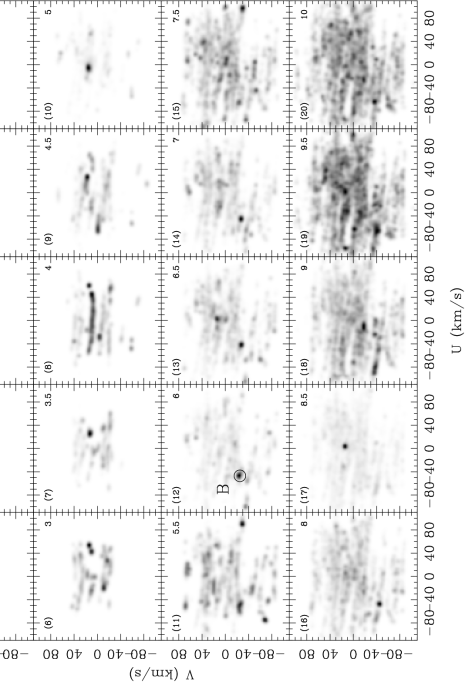
One of the striking features of the solar neighbourhood df is that the same moving groups appear to be present in stellar populations of different ages (see Table 2 of Dehnen 1998 or the top row of Figure 9). This result is difficult to understand in the traditional view that moving groups arise from inhomogeneous star formation. Thus it is worthwhile to explore the temporal evolution of the df and the survival of moving groups in our simulations.

Our standard four simulations, R₅, R₁₀, R₂₀, and R₄₀, are not ideal for this task. As we have seen, run R₅ has relatively weak moving groups and unrealistic parameters. The other runs show a strong moving group at the origin in the combined df  which is not present in the observed df. This moving group arises because the typical interval between spiral transients in these simulations is 0.5–1 Gyr (Table 1). Thus in most of these runs there has been no spiral transient in the last $\sim 0.5$ Gyr, and all of the stars formed since the last transient still have their birth epicycle energy, which is nearly zero. Moreover, these runs feature a relatively small number of strong spirals, which hit the disk very infrequently but hard. They may therefore overestimate the persistence of moving groups.

To address these concerns, we have run another simulation R_sim. In this run, we increase the number of spirals to $N_{s}=48$ and set $\epsilon=0.31$. We have also adjusted the central times of the spiral transients as follows: (1) We have set the central time $t_{s}$ of the most recent transient to be the present time $t_{0}$; (2) Because Dehnen’s subsample B1, in which the oldest stars have age 0.4 Gyr, already shows two prominent moving groups (top left panel of Figure 9), we have set the central time of another transient to $t_{0}-0.2$ Gyr; (3) The other central times are chosen randomly between $t_{s}=0$ and $t_{s}=t_{0}-0.2$ Gyr. This strategy suppresses the strong moving group at the origin and makes the other features in the df more prominent.

Figure 8 shows the velocity distribution in run R_sima as a function of stellar age. “Moving groups” (i.e. the same local concentration of stars in velocity space) can be seen among stars of any age, even the oldest stars. Generally with increasing age there are more but weaker moving groups, however, a strong “moving group” can be present even in a very old sample (see panel 17, 8.5 Gyr). Notice that the same “moving group” can be present in stars with a wide range of ages; for example, the moving group “B” in panel 13 can be traced from panels 11 to 14, a range of at least 1.5 Gyr in age. This result is consistent with the observation that the same moving group is seen in observational sub-samples of different age (e.g., Dehnen 1998, Table 2).

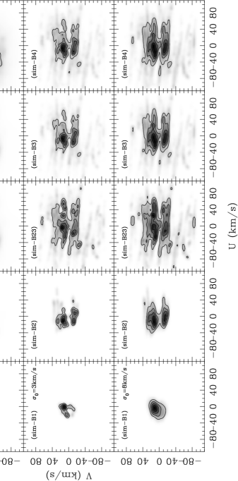
In Figure 9 we show the observed and simulated dfs, divided into age bins. The observed df, shown in the top row, is taken from Dehnen (1998). The panels represent subsamples determined by color cuts, which should correspond to age cuts. The maximum ages in the three subsamples B1, B2, and B3 (the first, second, and fourth panels) are 0.4 Gyr, 2 Gyr, and 8 Gyr (Table 1 of Dehnen 1998). The sample B4GI (fifth panel) is a combination of red ($B-V>0.6$) main-sequence stars and giant stars, which should have a uniform distribution of ages if the star-formation rate has been uniform. The third panel, labeled B23, is obtained by subtracting the scaled df of B2 from the df of B3, in order to represent approximately the df of stars with ages 2–8 Gyr.

In the bottom two rows of Figure 9 we show the simulated dfs from two runs: run R_sim, and a modified version of R_sim in which the width $\sigma_{0}$ of the epicycle energy at formation (eq. 15) is increased from $3{\rm\,km\,s^{-1}}$ to $8{\rm\,km\,s^{-1}}$. The different panels show the dfs corresponding to the same age ranges as in the subsamples of the data. The simulated dfs reproduce most of the prominent features of the observed dfs: (1) The stars clump together in moving groups. (2) The number of moving groups increases as the mean stellar age increases, from left to right in the figure. (3) The same moving groups are present in stars with a wide range of ages. (4) The moving groups appear to be elongated along lines of constant $v$, although this effect is significantly stronger in the simulations than the observations.

Increasing the initial epicycle energy (compare the second and third row of Figure 9) spreads out the moving groups somewhat, and enhances their elongation along lines of constant $v$, but they remain prominent; the moments of the df given in Table 2 are almost unchanged.

In Figure 10 we plot the birthplaces of groups “A” and “B” shown in panels 2 and 12 of Figure 8. The stars in the younger group, A (age 1 Gyr), come from a relatively small arc, while the stars in the older moving group B (age 6 Gyr) were born with a wide range of Galactic azimuths. In contrast, Eggen’s model for moving groups predicts that the stars in a group should be born in a small region and thus should have the same age and metallicity.

We also ran a modified version of R₂₀, which has the same parameters as R₂₀ but adjusts the central times of the transients as described above for R_sim. This run gives more prominent moving groups than R_sim, and the groups last for a longer time (up to 3.5 Gyr). This result suggests that a small number of strong spiral transients tend to produce strong moving groups and a lumpy df, while a large number of weak transients tend to produce weak or undetectable moving groups and a smooth df. Therefore, the observed moving groups suggest that at most a few tens of spiral transients have affected the stars in the solar neighbourhood.

We also looked for moving groups in run R_m4, which has the same parameters (including the random number seeds) as the modified run R₂₀, except that the spirals have four arms. We found that substructure in the df in run R_m4 was much weaker than in the modified run R₂₀, presumably because the wavelength $2\pi/k$ of the arms is smaller so the df is more thoroughly mixed for a given amount of heating. The absence of substructure suggests that transient spirals in the Galaxy may be predominantly two-armed rather than four-armed. Further exploration of the effects of the spiral-structure parameters on the structure of the local df is obviously worthwhile.

We have also looked for substructure in the velocity df in runs in which the duration $\sigma_{s}$ of the spiral transients was varied (Figure 3). We found that the strength of the substructure declines as $\sigma_{s}$ increases; in other words, spiral transients with duration much longer than $\Omega^{-1}$ tend to heat the disk without generating moving groups.

We have also investigated heating by gmcs rather than spiral structure, and find that this process does not yield significant substructure in the df (De Simone, 2000). Thus the observed strong substructure suggests that spiral structure rather than gmcs is the dominant heating mechanism in the solar neighbourhood, a conclusion reached by others from independent arguments (see §1).

Figure 8: The evolution of the velocity distribution as a function of age, from run R_sima. Each panel is labeled with the age in Gyr. The gray scale in each panel is relative to the maximum density in that panel. Notice that the moving group B can be seen at least from panels 7 to 13, corresponding to ages of 3.5–6.5 Gyr.

Figure 9: The observed df as a function of stellar age (Dehnen, 1998), compared to simulated dfs from run R_sima. From left to right, the samples represent stars younger than 0.4 Gyr, stars younger than 2 Gyr, stars from 2–8 Gyr in age, stars younger than 8 Gyr, and stars of all ages (see text for further details). The bottom row is from a run with the same parameters as R_sima except that initial dispersion ${\sigma_{0}}$ is $8{\rm\,km\,s^{-1}}$ rather than $3{\rm\,km\,s^{-1}}$.

Figure 10: The birthplaces of stars in moving groups “A” and “B” in Figure 8. The star shows the Galactic centre. The stars in a moving group are not born at a single location. The locations are obtained from the coordinates of the stars in the sheared sheet by equating the polar coordinates $R/R_{0}$ and $\phi$ to $1+x$ and $y$, respectively.

5 Inhomogeneous star formation

So far in this paper we have assumed that the star-formation rate is uniform in both space and time, and that both the avr and the structure of the velocity distribution in the solar neighbourhood are due to scattering by the large-scale potential fluctuations associated with transient spiral arms. The traditional view, which we explore briefly in this Section, is that the structure in the local velocity distribution results from spatial and temporal variations in the star-formation rate. Of course, some elements of both pictures must be correct, since we know both that spiral arms are present and that star formation is concentrated in gmcs.

The observed avr requires heating by some mechanism—whether spiral arms, gmcs, or one of the other mechanisms discussed in §1. However, in this Section we ignore the details of this heating, to focus on the properties of the irregularities in the velocity distribution that are due to inhomogeneous star formation alone. We consider the following crude model:

1. All stars form in clusters of $N$ stars, of limited spatial extent.

2. The cluster dissociates after the stars form. When the cluster dissociates, the df of its stars is Gaussian in both position and velocity, with dispersions $\sigma_{q}$ and $\sigma_{p}$ respectively. The stars do not interact with one another once the cluster has dissolved; thus, their motion is governed by equations (6). Typical values of $\sigma_{q}$ and $\sigma_{p}$ are a few pc or ${\rm\,km\,s^{-1}}$.

3. The heating mechanism does not disrupt or spread the phase-space stream of stars from the dissolved cluster (any such effects will make many of the conclusions below even stronger). We ignore the details of the heating mechanism, and account for heating by simply assuming that the dissociated cluster is born at position $(x_{0},y_{0})$, on a non-circular orbit with velocities $u_{0}$ and $v_{0}$. Thus, the initial df of the dissociated cluster is

   $$f_{0}({\bf z})={N\over(2\pi\sigma_{p}\sigma_{q})^{2}}\exp\left[-{\textstyle{1\over 2}}({\bf z}-{\bf z}_{0}){\bf Q}({\bf z}^{T}-{\bf z}_{0}^{T})\right].$$ (32)

   where ${\bf z}=(x,y,u,v)$, $T$ denotes the transpose, and

   $${\bf Q}=\left(\begin{array}[]{cccc}\sigma_{q}^{-2}&0&0&0\\ 0&\sigma_{q}^{-2}&0&0\\ 0&0&\sigma_{p}^{-2}&0\\ 0&0&0&\sigma_{p}^{-2}\\ \end{array}\right).$$ (33)

   The covariance matrix is

   $$\langle({\bf z}^{T}-{\bf z}_{0}^{T})\otimes({\bf z}-{\bf z}_{0})\rangle={\bf Q}^{-1},$$ (34)

   where the average $\langle\cdot\rangle$ is over the df $f_{0}({\bf z})$.

The trajectories (6) can be rewritten in the form (Asiain, Figueras & Torra, 1999)

$${\bf z}(t)={\bf A}(t){\bf z}(0),$$ (35)

where $t$ is the time elapsed since the dissociation of the cluster, and (recall that $u=-\dot{x}$)

$${\bf A}(t)=\left(\begin{array}[]{cccc}{\Omega-A\cos\tau\over\Omega-A}&0&-{\sin\tau\over\kappa}&{1-\cos\tau\over 2(\Omega-A)}\\ {2A\Omega(\sin\tau-\tau)\over\kappa(\Omega-A)}&1&{2\Omega(1-\cos\tau)\over\kappa^{2}}&{\Omega\sin\tau-A\tau\over\kappa(\Omega-A)}\\ -{A\kappa\sin\tau\over\Omega-A}&0&\cos\tau&-{\kappa\sin\tau\over 2(\Omega-A)}\\ {2A\Omega(\cos\tau-1)\over\Omega-A}&0&{2\Omega\sin\tau\over\kappa}&{\Omega\cos\tau-A\over\Omega-A}\\ \end{array}\right).$$ (36)

Here $\tau\equiv\kappa t$. The matrix ${\bf A}(t)$ has the following properties: ${\bf A}(0)={\bf I}$ (by definition), $|{\bf A}(t)|=1$ (by Liouville’s theorem), and ${\bf A}^{-1}(t)={\bf A}(-t)$ (by time-reversibility).

Since phase-space density is conserved along the particle trajectories, the initial df is Gaussian (eq. 32), and ${\bf z}(t)$ is a linear function of ${\bf z}(0)$, the df of the dissociated cluster will remain Gaussian for all time. The centroid of the Gaussian will be ${\bf z}_{c}(t)={\bf z}_{0}{\bf A}^{T}(t)$ and the covariance matrix will be

$${\bf C}(t)\equiv\langle[{\bf z}^{T}-{\bf z}_{c}^{T}(t)]\otimes[{\bf z}-{\bf z}_{c}(t)]\rangle={\bf A}(t){\bf Q}^{-1}{\bf A}^{T}(t).$$ (37)

The disrupted cluster is greatly elongated in the azimuthal direction. Therefore to estimate the maximum number of stars from a cluster that could be visible in the solar neighbourhood, it is useful to compute the linear number density at time $t$, $n(y,t)=\int f({\bf z},t)dx\,d{\bf v}$, where ${\bf z}=(x,y,u,v)=({\bf x},{\bf v})$. Since the df is Gaussian, the linear density must also be Gaussian,

$$n(y,t)={N\over(2\pi\sigma_{y}^{2})^{1/2}}\exp\left[-(y-y_{c})^{2}/2\sigma_{y}^{2}\right],$$ (38)

where

$$\sigma_{y}^{2}=\langle[y-y_{c}(t)]^{2}\rangle=C_{22}(t);$$ (39)

at large times, $\kappa t\gg 1$, we have (Asiain, Figueras & Torra, 1999)

$$\sigma_{y}\simeq{4A\Omega t\over\kappa^{2}}(\sigma_{p}^{2}+4\Omega^{2}\sigma_{q}^{2})^{1/2}.$$ (40)

For a typical star-forming cluster, $\Omega\sigma_{q}\ll\sigma_{p}$ ($\Omega\sigma_{q}=0.03{\rm\,km\,s^{-1}}(\sigma_{q}/1{\rm\,pc})$ compared to typical values $\sigma_{p}=1{\rm\,km\,s^{-1}}$). Thus we may drop the term involving $\sigma_{q}$, so the maximum linear density from a disrupted cluster of age $t$ is

$$n_{\rm max}(t)={N\over(2\pi)^{1/2}\sigma_{p}t}\left(\kappa^{2}\over 4A\Omega\right),$$ (41)

where the factor in brackets is unity for a flat rotation curve. In the solar neighbourhood,

$$n_{\rm max}(t)=4\times 10^{-5}{\rm\,pc}^{-1}N\left(1{\rm\,km\,s^{-1}}\over\sigma_{p}\right)\left(10{\rm\,Gyr}\over t\right).$$ (42)

With the same assumptions, the rms spatial extent of the cluster in the radial direction is

$$\sigma_{x}={\sigma_{p}\over\Omega}\left[{\textstyle{1\over 2}}\sin^{2}\kappa t+(1-\cos\kappa t)^{2}\right]^{1/2};$$ (43)

averaging over the epicycle period we have $\sigma_{x}=({7\over 4})^{1/2}\sigma_{p}/\Omega=50{\rm\,pc}(\sigma_{p}/1{\rm\,km\,s^{-1}})$.

Now suppose that our survey includes all stars in the solar neighbourhood to a distance $L$. Then if $L\ga\sigma_{x}$ we can detect up to $2n_{\rm max}L$ stars in the moving group, while if $L\ll\sigma_{x}$ we will detect up to $(\pi/2)^{1/2}n_{\rm max}L^{2}/\sigma_{x}$ stars in the group (these upper limits are achieved if the Sun lies exactly on the centroid $x_{c}(t)$). Extrapolating these formulas until they meet, we find that the upper limit to the number of detected stars in the moving group is given by

$$n_{\rm mg}<8\times 10^{-3}N{L\over 100{\rm\,pc}}{1{\rm\,km\,s^{-1}}\over\sigma_{p}}{10{\rm\,Gyr}\over t}$$ (44)

for $L>80{\rm\,pc}(\sigma_{p}/1{\rm\,km\,s^{-1}})$, and

$$n_{\rm mg}<1.0\times 10^{-2}N\left(L\over 100{\rm\,pc}\right)^{2}\left(1{\rm\,km\,s^{-1}}\over\sigma_{p}\right)^{2}{10{\rm\,Gyr}\over t}$$ (45)

for $L<80{\rm\,pc}(\sigma_{p}/1{\rm\,km\,s^{-1}})$. The sample of Dehnen (1998) was limited to distances $L\simeq 100{\rm\,pc}$ (the median parallax error in the Hipparcos catalog is $\sigma_{\pi}=1$ mas and Dehnen’s sample is restricted to stars with $\sigma_{\pi}/\pi\leq 0.1$). If we assume that at least $n_{\rm mg}=50$ stars are needed to define a moving group, then any such group identified in Dehnen’s catalog must have come from a cluster with initial population

$$N\ga 6\times 10^{3}{\sigma_{p}\over 1{\rm\,km\,s^{-1}}}{t\over 10{\rm\,Gyr}}\quad\hbox{if $\sigma_{p}<1.3{\rm\,km\,s^{-1}}$},$$ (46)

or

$$N\ga 5\times 10^{3}\left(\sigma_{p}\over 1{\rm\,km\,s^{-1}}\right)^{2}{t\over 10{\rm\,Gyr}}\quad\hbox{if $\sigma_{p}>1.3{\rm\,km\,s^{-1}}$}.$$ (47)

These are conservative lower limits, since (i) we have neglected the spreading of the stream due to interactions with small-scale fluctuations in the gravitational potential, such as gmcs; (ii) we have assumed that the radial coordinate of the stream of stars is centred precisely on the Sun.

Infrared observations show that most star formation occurs in embedded star clusters within gmcs. These clusters have masses in the range $50$–$10^{3}M_{\odot}$ (Lada & Lada, 2003) and virial dispersions $\sigma_{p}\sim 1{\rm\,km\,s^{-1}}$ and thus are too small to contribute detectable moving groups with an age exceeding $\sim 1{\rm\,Gyr}$. An alternative is to suppose that the dissociated cluster is the gmc itself. In this case $\sigma_{p}\sim 5{\rm\,km\,s^{-1}}$ which requires $N\ga 1.3\times 10^{5}$; given that the largest gmcs have gas masses $\sim 10^{5}$–$10^{6}M_{\odot}$ we would require extremely high star-formation efficiency to produce a sufficient number of stars. In other words it is difficult to find a plausible astrophysical source for the star-forming regions which are supposed to be the progenitors of the old moving groups.

6 Migration

Sellwood & Binney (2002) discuss the dynamics of radial migration due to transient spiral arms, and the relationship between radial migration and disk heating. They estimate that old stars formed in the solar neighbourhood should now be scattered nearly uniformly throughout the annulus from $R_{0}\pm 4{\rm\,kpc}$.

We have examined the radial migration or diffusion of stars that is induced by spiral-wave scattering, using the spiral-arm parameters for our runs R₅, R₁₀, R₂₀ and R₄₀. In each case we started 100,000 test stars in circular orbits near the solar neighbourhood ($\pm 0.2{\rm\,kpc}$) and followed them for 10 Gyr. In Figure 11 we plot the rms change in guiding-centre radius and the distribution of stars as functions of final epicycle energy. The present in-plane epicycle energy of the Sun is only $E_{x}=64({\rm\,km\,s^{-1}})^{2}$, which is nearly zero on the scale of these plots. If these simulations correctly represent the properties of the local spiral structure, we expect that the radial migration of the Sun since its formation 4.5 Gyr ago is in the range $0.45\pm 0.25{\rm\,kpc}$ (pitch angle $10\degr$) to $1.4\pm 0.9{\rm\,kpc}$ (pitch angle $20\degr$). The sheared sheet is symmetric in $\pm x$ so our simulations cannot address the question of whether the migration is likely to be inward or outward; Sellwood & Binney (2002) argue that migration is generally outward because of the surface-density gradient in the disk. These estimates of the migration are consistent with the estimate made by Wielen, Fuchs & Dettbarn (1996), on the basis of the Sun’s metallicity and the radial metallicity gradient in the Galactic disk, that the Sun has migrated outward by $1.9\pm 0.9{\rm\,kpc}$ in the past 4.5 Gyr.

Figure 11: (top) The mean of $|\Delta R|$, the absolute value of the change in guiding-centre radius, as a function of final epicycle energy $E_{x}=\frac{1}{2}\kappa^{2}a^{2}$, where $a$ is the epicycle amplitude (eq. 10). The stars are initially in circular orbits with radius $R_{0}$. The four panels correspond to scattering by spiral arms with the parameters of runs R₅, R₁₀, R₂₀ and R₄₀ (Table 1). The error bars represent the standard deviation in the distribution of $|\Delta R|$ at a given radial energy. (bottom) The distribution of stars as a function of epicycle energy. Dashed lines are the Schwarzschild distribution with the same velocity dispersion.

7 Discussion

We have explored the hypothesis that transient spiral arms are the dominant mechanism that drives the evolution of the velocity distribution in the solar neighbourhood (Barbanis & Woltjer, 1967; Sellwood & Carlberg, 1984; Carlberg & Sellwood, 1985). The most thorough investigations of this mechanism so far have been based on the Fokker-Planck equation (Jenkins & Binney, 1990; Jenkins, 1992). Our investigation is based on direct numerical integration of test-particle orbits in the sheared sheet (eqs. 3). We impose a randomly distributed sequence of trailing $m=2,4$ spiral waves with pitch angle $\alpha$ and a strength that is Gaussian in time (eq. 21), and apply the boundary conditions that the test particles must be on circular orbits at their formation time and in the solar neighbourhood at the present time.

We confirm that transient spiral waves can heat the galactic disk in velocity space. The configurations of the spiral waves in our simulations, such as the number ($N_{s}=9$–48), duration ($\Omega\sigma_{s}=0.5$–2.5), rms fluctuation amplitude ($\epsilon_{\caps rms}=0.16$–0.86), and pitch angle ($\alpha=5\degr$–$40\degr$) are all plausible. Spiral arms can lead to a wide range in the observed exponent of the age-velocity dispersion relation (eq. 29), $p=0.2$–0.76, so this exponent is not a strong discriminator between different mechanisms of disk heating. The variations of the vertex deviation, mean radial velocity, and axis ratios of the velocity ellipsoid in the solar neighbourhood are consistent with observations.

The small-scale structure of the local stellar velocity distribution cannot be interpreted in terms of axisymmetric, steady-state models. Our simulated distribution functions do not have the Schwarzschild form (1) and in addition exhibit rich small-scale structure, similar to the “moving groups” and “branches” that observers describe in the solar neighbourhood distribution function. This result suggests that moving groups arise primarily from smooth star formation in a lumpy potential, in contrast to the traditional assumption that they reflect lumpy star formation in a smooth potential—although of course elements of both pictures must be present to some extent.

All these findings strongly support the conclusion that transient spiral waves are the dominant heating mechanism of the disk in the solar neighbourhood.

Strong substructure in the local velocity distribution is most easily produced when the Galaxy experiences a small number of short-lived but strong (fractional surface-density amplitude $\epsilon\sim 1$) spiral transients, as might be caused by minor mergers. A model in which spiral transients are continuously present at a lower amplitude could reproduce the age-velocity dispersion relation without significant substructure.

We also find some other results:

1. The age-velocity dispersion relation depends strongly on the stochastic properties of the spiral waves, especially in cases where the heating is due mainly to a relatively small number of spiral transients (e.g. $\sim 10$ in runs R₂₀ and R₄₀). Therefore, it is difficult, if not impossible, to infer the details of the heating mechanism from observations of the age-velocity dispersion relation, no matter how accurate.

2. Spiral arms lead to radial migration of stars (Sellwood & Binney 2002 and references therein). For the spiral-wave parameters we used, the rms radial migration of a star like the Sun is a strong function of pitch angle $\alpha$, ranging from $0.45\pm 0.25{\rm\,kpc}$ for $\alpha=10\degr$ to $1.4\pm 0.9{\rm\,kpc}$ for $\alpha=20\degr$. In other words the relation between the amount of heating of the solar neighborhood and the amount of radial migration is not unique, a conclusion already reached by Sellwood & Binney (2002) using other arguments.

3. Stars in old moving groups did not form at a common place and time, and therefore do not necessarily share a common age and metallicity.

4. The traditional model, in which structure in the velocity distribution function is the result of inhomogeneous star formation, is difficult to reconcile with at least two observations: 1. In this model, all of the stars in a moving group should have the same age and metallicity, while in fact the stars in prominent moving groups show a wide range of ages. 2. It is difficult to find a suitable astrophysical source that is small enough, cold enough, and produces enough stars to be the progenitor of the old moving groups.

5. We have also investigated heating by giant molecular clouds alone, and find that this process produces much weaker substructure in the distribution function than is observed (De Simone, 2000); thus giant molecular clouds are unlikely to be the dominant heating mechanism in the solar neighbourhood.

Although heating by spiral waves explains most of the properties of the solar neighbourhood velocity distribution, there is still room for other heating mechanisms, such as the Galactic bar, giant molecular clouds, and halo substructure or minor mergers.

8 Acknowledgments

We thank James Binney, Walter Dehnen, and Jerry Sellwood for discussions and advice, and the referee, Agris Kalnajs, for many insightful comments. This research was supported in part by NSF Grant AST-9900316.

References

- Asiain, Figueras & Torra (1999) Asiain R., Figueras F., Torra J. 1999, A&A, 350, 434
- Barbanis & Woltjer (1967) Barbanis B., Woltjer L., 1967, ApJ, 150, 461
- Binney & Lacey (1988) Binney J., Lacey C., 1988, MNRAS, 230, 597
- Binney & Merrifield (1998) Binney J., Merrifield M., 1998, Galactic Astronomy. Princeton University Press, Princeton
- Binney & Tremaine (1987) Binney J., Tremaine S., 1987, Galactic Dynamics. Princeton University Press, Princeton
- Binney, Dehnen & Bertelli (2000) Binney J., Dehnen W., Bertelli G., 2000, MNRAS, 318, 658
- Block & Puerari (1999) Block D. L., Puerari, I., 1999, A&A, 342, 627
- Carlberg (1987) Carlberg R. G., 1987, ApJ, 322, 59
- Carlberg & Sellwood (1985) Carlberg R. G., Sellwood J. A., 1985, ApJ, 292, 79
- Carlberg et al. (1985) Carlberg R. G., Dawson P. C., Hsu T., VandenBerg D. A., 1985, ApJ, 294, 674
- Chandrasekhar (1942) Chandrasekhar S., 1942, Principles of Stellar Dynamics (Chicago: University of Chicago Press)
- Chereul, Crézé, & Bienaymé (1998) Chereul E., Crézé M., Bienaymé O. 1998, A&A, 340, 384
- Chereul, Crézé, & Bienaymé (1999) Chereul E., Crézé M., Bienaymé O. 1999, A&AS, 135, 5
- Crézé et al. (1998) Crézé M., Chereul E., Bienaymé O., Pichon C. 1998, A&A, 329, 920
- De Simone (2000) De Simone R., 2000, AB thesis, Princeton University
- de Zeeuw et al. (1999) de Zeeuw, P. T., Hoogerwerf, R., de Bruijne, J.H.J., Brown, A.G.A., Blaauw, A., 1999, AJ, 117, 354
- Dehnen (1998) Dehnen W., 1998, AJ, 115, 2384
- Dehnen (1999) Dehnen W., 1999, ApJ, 524, L35
- Dehnen (2000) Dehnen W., 2000, AJ, 119, 800
- Dehnen & Binney (1998) Dehnen W., Binney, J., 1998, MNRAS, 298, 387
- Drimmel (2000) Drimmel R., 2000, A&A, 358, L16
- Eggen (1996) Eggen O. J., 1996, AJ, 112, 1595
- Elmegreen (1998) Elmegreen D. M., 1998, Galaxies and Galactic Structure (Prentice-Hall: Upper Saddle River)
- Elmegreen et al. (1999) Elmegreen D. M., Chromey F. R., Bissell B. A., Corrado K., 1999, AJ, 118, 2618
- Freeman (1991) Freeman K. C., 1991, in Sundelius B., ed., Dynamics of Disc Galaxies. Göteborgs University, Göteborg, p. 15
- Fux (2001) Fux R., 2001, A&A, 373, 511
- Goldreich & Lynden-Bell (1965) Goldreich P., Lynden-Bell D., 1965, MNRAS, 130, 125
- Gómez et al. (1997) Gómez A., Grenier S., Udry S., Haywood M., Meillon L., Sabas V., Sellier A., Morin D., 1997, in Battrick B., ed. Hipparcos – Venice ’97, ESA SP-402. European Space Agency, Noordwijk, p. 621
- Holmberg & Flynn (2000) Holmberg J., Flynn C., 2000, MNRAS, 313, 209
- Huang & Carlberg (1997) Huang S., Carlberg R. G., 1997, ApJ, 480, 503
- Ida, Kokubo & Makino (1993) Ida S., Kokubo E., Makino J., 1993, MNRAS, 263, 875
- James & Seigar (1999) James, P. A., Seigar, M. S., 1999, A&A, 350, 791
- Jenkins (1992) Jenkins A., 1992, MNRAS, 257, 620
- Jenkins & Binney (1990) Jenkins A., Binney J., 1990, MNRAS, 245, 305
- Julian & Toomre (1966) Julian W. H., Toomre A., 1966, ApJ, 146, 810
- Kalnajs (1991) Kalnajs A. J., 1991, in Sundelius, B., ed., Dynamics of Disc Galaxies. Göteborgs University, Göteborg, p. 323
- Kapteyn (1905) Kapteyn J. C., 1905, Brit. Assoc. Report, 257
- Korchagin et al. (2003) Korchagin V. I., Girard T. M., Borkova T. V., Dinescu D. I., van Altena W. F. 2003, astro-ph/0308276
- Lacey (1984) Lacey C. G., 1984, MNRAS, 208, 687
- Lacey (1991) Lacey C. G., 1991, in Sundelius, B., ed., Dynamics of Disc Galaxies. Göteborgs University, Göteborg, p. 257
- Lacey & Ostriker (1985) Lacey C., Ostriker J. P., 1985, ApJ, 299, 633
- Lada & Lada (2003) Lada C. J., Lada E. A. 2003, ARAA, 41, in press
- Lynden-Bell & Kalnajs (1972) Lynden-Bell D., Kalnajs A. J., 1972, MNRAS, 157, 1
- Ma et al. (1999) Ma J., Zhao J. L., Shu C. G., Peng Q. H., 1999, A&A, 350, 31
- Quillen (2003) Quillen A., 2003, AJ, 125, 785
- Quillen & Garnett (2001) Quillen A. C., Garnett D. R., 2001, in Galaxy Disks and Disk Galaxies, J. G. Funes & E. M. Corsini, eds. (San Francisco: Astronomical Society of the Pacific), 87
- Rhoads (1998) Rhoads J. E., 1998, AJ, 115, 472
- Rix & Rieke (1993) Rix H.-W., Rieke M. J., 1993, ApJ, 418, 123
- Rix & Zaritsky (1995) Rix H.-W., Zaritsky D., 1995, ApJ, 447, 82
- Schwarzschild (1907) Schwarzschild K., 1907, Göttingen Nachr. 1907, 614
- Seigar & James (1998) Seigar M. S., James P. A.,1998, MNRAS, 299, 685
- Sellwood (1999) Sellwood J. A., 1999, in Galaxy Dynamics, ed. D. Merritt, J. A. Sellwood & M. Valluri (San Francisco: Astronomical Society of the Pacific), 351
- Sellwood & Carlberg (1984) Sellwood J. A., Carlberg R. G., 1984, ApJ, 282, 61
- Sellwood & Binney (2002) Sellwood J. A., Binney, J. J., 2002, MNRAS, 336, 785
- Skuljan, Hearnshaw & Cottrell (1999) Skuljan J., Hearnshaw J. B., Cottrell P. L., 1999, MNRAS, 308, 731
- Spitzer & Schwarzschild (1951) Spitzer L., Schwarzschild M., 1951, ApJ, 114, 385
- Spitzer & Schwarzschild (1953) Spitzer L., Schwarzschild M., 1953, ApJ, 118, 106
- Tóth & Ostriker (1992) Tóth G., Ostriker J. P., 1992, ApJ, 389, 5
- Toomre & Kalnajs (1991) Toomre, A., & Kalnajs A. J., 1991, in Sundelius, B., ed., Dynamics of Disc Galaxies. Göteborgs University, Göteborg, p. 341
- Vallée (2002) Vallée J. P., 2002, ApJ, 566, 261
- Villumsen (1985) Villumsen J. V., 1985, ApJ, 290, 75
- Walker, Mihos & Hernquist (1996) Walker I. R., Mihos J. C., Hernquist L., 1996, ApJ, 460, 121
- Wielen, Fuchs & Dettbarn (1996) Wielen R., Fuchs B., Dettbarn C., 1996, A&A, 314, 438
- Woolley (1961) Woolley R., 1961, The Observatory, 81, 203