Correlated Hybrid Fluctuations from Inflation with Thermal Dissipation

Abstract

We investigate the primordial scalar perturbations in the thermal dissipative inflation where the radiation component (thermal bath) persists and the density fluctuations are thermally originated. The perturbation generated in this model is hybrid, i.e. it consists of both adiabatic and isocurvature components. We calculate the fractional power ratio ($S$) and the correlation coefficient ($\cos\Delta$) between the adiabatic and the isocurvature perturbations at the commencing of the radiation regime. Since the adiabatic/isocurvature decomposition of hybrid perturbations generally is gauge-dependent at super-horizon scales when there is substantial energy exchange between the inflaton and the thermal bath, we carefully perform a proper decomposition of the perturbations. We find that the adiabatic and the isocurvature perturbations are correlated, even though the fluctuations of the radiation component is considered uncorrelated with that of the inflaton. We also show that both $S$ and $\cos\Delta$ depend mainly on the ratio between the dissipation coefficient $\Gamma$ and the Hubble parameter $H$ during inflation. The correlation is positive ($\cos\Delta>0$) for strong dissipation cases where $\Gamma/H>0.2$, and is negative for weak dissipation instances where $\Gamma/H<0.2$. Moreover, $S$ and $\cos\Delta$ in this model are not independent of each other. The predicted relation between $S$ and $\cos\Delta$ is consistent with the WMAP observation. Other testable predictions are also discussed.

I Introduction

The recently released data of the Wilkinson Microwave Anisotropy Probe (WMAP) confirmed the earlier COBE-DMR’s observation about the deficiency in fluctuation power at the largest angular scales wmap ; dmr4 . The amount of quadrupole and octopole modes of the CMB temperature fluctuations is anomalously low if compared to the prediction of the $\Lambda$CDM model. It implies that the initial density perturbations are significantly suppressed on scales equal to or larger than the Hubble radius. Models of structure formation with a cut-off power spectrum of perturbation on large scales provide a better fit to the CMB temperature fluctuations. The most likely cut-off wavelength derived from the WMAP data bri actually is the same as that determined by the COBE-DMR fj ; bfh .

The super-horizon suppression is difficult to make compatible with models which produce pure adiabatic (isentropic) perturbations. However, it might be explained if the perturbations are hybrid. The different behavior of adiabatic and isocurvature (entropic) perturbations around the horizon scale can be used to construct power spectra with a super-horizon suppression. The WMAP data show not only a possible non-zero fraction of isocurvature fluctuations in the primordial density perturbations, also the correlation between the adiabatic and the isocurvature components pei . These results then turn into the constraints on the multi-component inflationary models, as the initial perturbations generated from these models are principally hybrid kps . The double and multi-field models have been extensively studied in this context double .

In this paper we will investigate the hybrid perturbations created by an inflation with thermal dissipation, the warm inflation scenario bf . In the scheme of the thermal dissipative inflation the universe contains a scalar field and a thermal bath during the inflation era. The two components are coupled via the thermal dissipation. In addition to fitting the amplitude and the power law index of the power spectrum given by the COBE data lf1 , the thermal dissipative inflation leads to a super-horizon suppression of the perturbations by a factor $\geq 0.5$ lf3 . Recently, it has been found that the warm inflation of a spontaneous symmetry breaking potential with strong dissipation is capable of accommodating a running spectral index $n$ of the primordial perturbations, and generally yields $n>1$ on large scales and $n<1$ on small scales hall . Our purpose here is to study the fractional power of the isocurvature perturbations, as well as the cross correlation between the adiabatic and the isocurvature fluctuations in the thermal dissipative inflationary model.

In contrast to a single or a double field inflations, the evolution of the universe in the thermal dissipative inflation does not need a stage of non-thermal post-inflationary reheating. As long as the damping coefficent $\Gamma$ satisfies the criterion given in  lf1 , $\Gamma>(M/m_{\rm Pl})^{4}H$, where $m_{\rm Pl},\ M$, and $H$ stand for the Planck energy, the energy scale, and the Hubble expansion of the inflaton respectively, the dissipation is effective enough to make the temperature of the radiation component increase continuously during the inflationary epoch. The universe would eventually enter the radiation-dominated phase when the temperature is high enough so that the radiation component prevails. Since the evolution of entropy only depends upon the thermal dissipative process during inflation, the entropic perturbations are not contaminated by the entropy production in the reheating stage. Therefore, the primordial hybrid perturbations induced by the thermal dissipation can be calculated unambiguously.

The dynamical background of the thermal dissipative inflation model has been investigated within the framework of quantum field theory. It has been shown that the dissipation may amount to the coupling of the inflaton to a large number of particle species linde ; ber3 . In this sense, the two-field model and the thermal dissipation model can be considered as two extremes among multi-component inflations. The former adds one more field to the single inflaton, while the later has a large number of additional fields.

The adiabatic and the isocurvature perturbations in the thermal dissipative model have been estimated in lf2 ; tb . Yet, these calculations are not immune from the problems induced by gauge issues which are crucial for thermal dissipative perturbations lee . In particular when interactions between the inflaton and the thermal bath are substantial, the commonly used adiabatic/isocurvature decomposition is not gauge-independent on the ground of super-horizon. Therefore, we must take a full relativistic treatment to analyze the evolution of the hybrid perturbations generated in the thermal dissipative inflation. Moreover, the fluctuations of the radiation component have not been carefully considered in previous works. Although the energy fluctuations of the radiation component are always less than that of the inflaton field, they are not negligible in examining the relative phase between the adiabatic and the isocurvature perturbations.

This paper is organized as follows. In §II we introduce the thermal dissipative inflationary model in relativistic covariant form. The initial adiabatic-to-isocurvature ratio is given in §III. Sec. IV presents a full relativistic calculation on the super-horizon evolution of adiabatic and isocurvature perturbations. The numerical result of the spectrum of the adiabatic-to-isocurvature ratio is also given in §IV. We then summarize our findings in §V. The appendices provide the necessary details of the relativistic theory of linear perturbations.

II The models of thermal dissipative inflation

II.1 The background field and radiation

We consider a universe consisting of a scalar inflaton field $\phi$, and a radiation component which mimics the thermal bath. The total energy-momentum tensor is

$$T_{ab}=T_{(\phi)ab}+T_{(r)ab},$$ (1)

where subscripts $(\phi)$ and $(r)$ are respectively for the scalar field and the radiation, and the Latin indices run from 1 to 4.

The energy-momentum tensor can be decomposed into fluid quantities as el

$$T_{ab}=\rho u_{a}u_{b}+ph_{ab}+q_{a}u_{b}+q_{b}u_{a}+\pi_{ab},$$ (2)

in which $q_{a}u^{a}=\pi_{ab}u^{b}=0$, $\pi_{ab}=\pi_{ba}$, and $u_{a}$ can be any timelike vector field, i.e. $u^{a}u_{a}=-1$, which is generally taken to be the average velocity vector. The total energy density of matter measured by an observer $u^{a}$ is represented by $\rho$, while $p$ and $\pi_{ab}$ denote the isotropic and anisotropic pressures respectively. The quantity $q_{a}$ prescribes the energy flux relative to $u^{a}$.

With $u_{a}$, the line element of the spacetime can be written as

$$ds^{2}\equiv g_{ab}dx^{a}dx^{b}=-\left(u_{a}dx^{a}\right)^{2}+h_{ab}dx^{a}dx^{b},$$ (3)

where $h_{ab}\equiv g_{ab}+u_{a}u_{b}$ is a projection tensor which maps points into the rest space of the observer $u^{a}$. Hence at the space-time point $x^{a}$, the observer $u^{a}$ assigns to the event $x^{a}+dx^{a}$ a spatial separation $(h_{ab}dx^{a}dx^{b})^{1/2}$, and a time separation $u_{a}dx^{a}$ from him.

For a minimally coupled scalar field $\phi$, the Lagrangian is

$$L=\frac{1}{2}\partial^{a}\phi\partial_{a}\phi-V(\phi),$$ (4)

where $V(\phi)$ is a self-interaction potential. The fluid quantities of the energy-momentum tensor for the $\phi$ field are then

$$\rho_{(\phi)}=\frac{1}{2}(\phi,_{a}u^{a})^{2}+V(\phi), \ \ \ p_{(\phi)}=\frac{1}{2}(\phi,_{a}u^{a})^{2}-V(\phi),$$ (5)

$$q_{(\phi)a}=-\phi,_{c}u^{c}h^{b}_{a}\phi_{,b}, \ \ \ \pi_{(\phi)ab}=0.$$

Assuming the radiation component is a relativistic ideal fluid, we have

$$\rho_{(r)}=\kappa T^{4}, \ \ \ p_{(r)}=(1/3)\rho_{(r)},\ \$$ (6)

$$q_{(r)a}=0, \ \ \ \pi_{(r)ab}=0,$$

where $T$ is temperature, $\kappa=(\pi^{2}/30)g_{\rm eff}$ and $g_{\rm eff}$ is the effective number of degrees of freedom at temperature $T$. As mentioned previously, the thermal dissipative inflation is a multi-component model with very high multiplication, the parameter $g_{\rm eff}$ amounts to the actual number of components. For simplicity, we will absorb the factor $\kappa$ into $T$, and use $\rho_{(r)}=T^{4}$ in what follows.

II.2 Interactions between the scalar field and the thermal bath

The total energy-momentum conservation of the system is governed by

$$T^{ab}_{~{}~{};b}=0.$$ (7)

The interactions between the $\phi$ field and the thermal bath are characterized by the force vectors defined as

$$Q_{(\phi)a}\equiv T_{(\phi)a;b}^{~{}~{}b},\hskip 17.07164ptQ_{(r)a}\equiv T_{(r)a;b}^{~{}~{}b},$$ (8)

Obviously, we have

$$Q_{(\phi)a}+Q_{(r)a}=0.$$ (9)

The interaction term $Q_{(i)a}$ ($i$ is for $\phi$ or $r$) can be further decomposed into

$$Q_{(i)a}\equiv Q_{(i)}u_{a}+J_{(i)a}\hskip 17.07164pt{\rm and}\hskip 17.07164ptu^{a}J_{(i)a}=0.$$ (10)

The quantities $Q_{(i)}$ and $J_{(i)a}$ are, respectively, the temporal and the spatial components of $Q_{(i)a}$. They describe the energy and the momentum exchange between the scalar field and the thermal bath. Substituting (10) into (8), one has

$$Q_{(i)}=-u^{a}T_{(i)a;b}^{b}\hskip 17.07164ptJ_{(i)c}=h_{c}^{a}T_{(i)a;b}^{b}.$$ (11)

The dissipation of the scalar field can be modeled by

$$Q_{(\phi)a}=-Q_{(r)a}=-\Gamma(\phi_{,b}u^{b})\phi_{,a},$$ (12)

where $\Gamma$ can be a function of $\phi$, and is always positive. With Eq. (10) we have

$$Q_{(\phi)}=-Q_{(r)}=-\Gamma(\phi_{,a}u^{a})^{2},$$ (13)

and

$$J_{(\phi)c}=-J_{(r)c}=-\Gamma(\phi_{,b}u^{b})\phi_{,a}h_{c}^{a}.$$ (14)

III The Initial adiabatic and isocurvature perturbations

III.1 The background solutions

To find the background solutions, we consider all quantities being uniform and isotropic. Accordingly, the space-time of the universe assumes the flat Friedman-Robertson-Walker metric,

$$ds^{2}=\bar{g}_{ab}dx^{a}dx^{b}=-dt^{2}+a^{2}\left[dr^{2}+r^{2}\left(d\theta^{2}+\sin^{2}\theta d\phi^{2}\right)\right].$$ (15)

The Einstein equations of the expanding universe yield

$$\dot{H}=-4\pi G\left(\dot{\phi}^{2}+\gamma\rho_{(r)}\right),$$ (16)

and

$$H^{2}=\frac{8\pi G}{3}\left[\rho_{(r)}+\frac{1}{2}\dot{\phi}^{2}+V(\phi)\right],$$ (17)

where $\gamma=4/3$ represents the adiabatic index of the thermal radiation, $a$ denotes the cosmic scale factor, and $H=\dot{a}/a$ is the Hubble parameter.

The equation of motion for the scalar field $\phi$ is

$$\ddot{\phi}+3H\dot{\phi}+\Gamma\dot{\phi}-a^{-2}\nabla^{2}\phi+V_{,\phi}(\phi)=0.$$ (18)

For the uniform background field $\phi$, the $\nabla^{2}\phi$ term in (19) can be ignored, and we have

$$\ddot{\phi}+(3H+\Gamma)\dot{\phi}+V^{\prime}(\phi)=0.$$ (19)

where the $\prime$ denotes $\partial/\partial\phi$.

The equation of motion for the radiation component (the thermal bath) is derived from the first law of thermodynamics as

$$\dot{\rho}_{(r)}+3H\gamma\rho_{(r)}=\Gamma\dot{\phi}^{2}.$$ (20)

Thus, the quantity $\Gamma$ in (12) represents the dissipation “coefficient”, which describes the production of radiation from the $\phi$ field. Furthermore, for the background solution, Eq. (14) gives

$$J_{(\phi)c}=J_{(r)c}=0.$$ (21)

This is expected as the uniform and isotropic scalar field comoves with the radiation field, the net momentum exchange between them vanishes.

When the potential energy $V$ is dominant, i.e. $V\gg\rho_{(r)}+\frac{1}{2}\dot{\phi}^{2}$, the Hubble parameter $H(t)$ depends largely on $V$, and the universe undergoes an inflation. In the slow-roll regime $V^{\prime\prime}\ll 3H^{2}$, Eq. (19) yields

$$\dot{\phi}\simeq-\frac{V^{\prime}}{3H+\Gamma}.$$ (22)

The scalar field approximates the trajectory

$$\phi=\phi_{0}e^{\beta t}$$ (23)

with $\beta\simeq-V^{\prime\prime}(0)/(3H+\Gamma)\ll H$. Thus, with Eqs. (19) and (20), the behavior of the radiation component at the inflationary phase can be characterized by

$$T^{4}\equiv\rho_{(r)}\simeq\frac{\Gamma\beta^{2}}{4H}\phi^{2}\simeq\frac{\Gamma}{4H}\dot{\phi}^{2}.$$ (24)

This solution actually can be obtained directly from (20) by considering the slow rolling condition $\dot{\rho}_{(r)}\simeq 0$ bf . Hence, Eq. (24) is still true even when $\Gamma$ is $\phi$-dependent. Numerical solutions to Eqs. (19) and (20) show that (24) is indeed available when $\Gamma$ is a power law function of $\phi$ lf1 .

Thus, the temperature of the thermal bath increases mostly during the inflation era. In the standard inflation scenario which corresponds to the $\Gamma=0$ case, the radiation is blown off as $\exp(-4Ht)$. Therefore, the solution [Eq. (24)] is independent of the initial value of $\rho_{(r)}$ when $t$ is greater than $1/H$.

Equations (19) and (20) imply that the $\phi$ field dissipation would eventually heat up the universe, giving rise to the co-existence of the scalar field and a radiation component with temperature larger than the Hawking temperature, i.e.

$$T>H.$$ (25)

Under this condition, the large scale reheating is unnecessary for inflation with dissipation. That is, the inflation regime will smoothly transfer to the radiation-dominated regime when $T$ is high enough, and the radiation component becomes dominant bf . Numerical solutions to (19) and (20) have shown the smooth transition lf1 . This feature is critical for calculating the primordial entropic fluctuations because the initial perturbations will be unaffected by the large scale post-inflationary entropic process, such as the reheating.

III.2 Initial perturbations of the scalar field

The initial perturbations of the $\phi$ field is calculated by the linearly perturbed field equation upon the space-time background (15). Because the primordial fluctuations are produced well within the Hubble radius, one can use the calculation without considering the gravitational gauge lf1 . For instance, the Fourier mode of the $\phi$ field perturbations with comoving wavenumber $k$ is characterized by a Langevin-like equation

$$\frac{d\delta\phi}{dt}=-\frac{k^{2}a^{-2}+V^{{}^{\prime\prime}}(\phi)}{3H+\Gamma}\delta\phi+\eta.$$ (26)

The noise term $\eta$ given by thermal fluctuations is Gaussian. The statistical property of the noise $\eta$ can be determined by means of the fluctuation-dissipation relation bf

$$\langle\eta\rangle=0,$$ (27)

$$\langle\eta({\bf k},t)\eta({\bf k^{\prime}},t^{\prime})\rangle=D\delta_{\bf k,-k^{\prime}}\delta(t-t^{\prime}),$$ (28)

with $D=(3H^{3}T/2\pi)(3H+\Gamma)^{-1}$, and $\langle...\rangle$ denotes averaging over an ensemble. The relation that $D=(H^{3}/2\pi)$ for the quantum case without dissipation is easily recovered.

Taking the slow-roll condition $|V^{{}^{\prime\prime}}(\phi)|\ll 9H^{2}$ into account, the $V^{{}^{\prime\prime}}(\phi)$ term in Eq. (26) can be ignored at the horizon-crossing where $a/k=H^{-1}$. Accordingly, the correlation function of the fluctuations is given by

$$\langle\delta\phi(t)\delta\phi(t^{\prime})\rangle\simeq D\frac{3H+\Gamma}{2H^{2}}e^{-(t-t^{\prime})H^{2}/(3H+\Gamma)},\ \ \ t>t^{\prime},$$ (29)

and the amplitude for the horizon sized perturbation $\delta\phi$ is about

$$\delta\phi\simeq\left(\frac{3}{4\pi}HT\right)^{1/2},$$ (30)

which implies the thermal fluctuations dominate over the quantum ones in the era of $T>H$. Taking the ensemble average, we obtain the perturbation $\delta\dot{\phi}$ just outside the horizon as

$$\delta\dot{\phi}\simeq-\frac{H^{2}}{3H+\Gamma}\delta{\phi}.$$ (31)

The perturbations in the $\phi$ field energy density is then

$$\delta\rho_{(\phi)}=\dot{\phi}\delta\dot{\phi}+V^{\prime}\delta\phi\simeq V^{\prime}\delta\phi=-(3H+\Gamma)\dot{\phi}\delta\phi\simeq-\left[2(\Gamma_{H}+3)\Gamma_{H}^{-1/2}\right]\cdot HT^{2}\delta\phi,$$ (32)

where we have used the slow-roll condition (22), and $\Gamma_{H}\equiv\Gamma/H$.

III.3 Initial perturbations of the thermal bath

We consider the radiation component in thermal equilibrium with a temperature $T$. At sub-horizon scales, fluctuations in the thermal radiation can be estimated by $\delta\rho_{(r)}/\rho_{(r)}\simeq 1/\sqrt{n_{r}}$ landau , where $n_{r}$ denotes the total number of the relativistic particles within the horizon $H^{-1}$. Since the photon number density is proportional to $T^{3}$, and the volume within the Hubble radius is about $(4\pi/3)H^{-3}$, we find that

$$\frac{\delta\rho_{(r)}}{\rho_{(r)}}\simeq\sqrt{\frac{3}{4\pi}}\left(\frac{H}{T}\right)^{3/2}.$$ (33)

Accordingly, the energy fluctuations caused by $\delta\rho_{(r)}$ are characterized by

$$\delta\rho_{(r)}\sim\frac{\delta\rho_{(r)}}{\rho_{(r)}}T^{4}\simeq\sqrt{\frac{3}{4\pi}HT}\cdot HT^{2}=HT^{2}\delta\phi,$$ (34)

where Eq.(30) has been used. It should be emphasized that (34) qualifies only the relation between the variances of $\delta\rho_{(r)}$ and $\delta\phi$, but not their phases. Principally thermal fluctuations of radiation component is random-phased with respect to the $\phi$ field fluctuations, i.e. $\langle\delta\phi\delta\rho_{(r)}\rangle=0$.

With the help of the background solutions (22) and (24), the relation between the fluctuations in the thermal energy and the $\phi$ field energy can be established,

$$\delta\rho_{(r)}=\delta\rho_{(\phi)}\frac{HT^{2}}{V^{\prime}(\phi)}=\frac{\Gamma_{H}^{1/2}}{2(\Gamma_{H}+3)}\delta\rho_{(\phi)}.$$ (35)

Therefore, $\delta\rho_{(r)}$ is always less than $\delta\rho_{(\phi)}$ in situations either $\Gamma<H$ or $\Gamma>H$. Apparently, the perturbed cosmic matter is just about isothermal.

III.4 The adiabatic vs. the isocurvature initial conditions

The energy perturbations of the $\phi$ field and the radiation component can be decomposed into adiabatic (ad) and isocurvature (en) modes as

$$\delta\rho_{(\phi)} = \delta\rho_{(\phi)}^{\rm ad}+\delta\rho_{(\phi)}^{\rm en},$$ (36)

$$\delta\rho_{(r)} = \delta\rho_{(r)}^{\rm ad}+\delta\rho_{(r)}^{\rm en}.$$ (37)

By definition, the adiabatic perturbations $\delta^{\rm ad}$ are given by

$$\delta^{\rm ad}=\frac{\delta\rho_{(\phi)}^{\rm ad}}{\rho_{(\phi)}+p_{(\phi)}}=\frac{\delta\rho_{(r)}^{\rm ad}}{\rho_{(r)}+p_{(r)}},$$ (38)

while the isocurvature mode satisfies

$$\delta\rho_{(\phi)}^{\rm en}+\delta\rho_{(r)}^{\rm en}=0.$$ (39)

Therefore, the adiabatic perturbations can be rewritten as

$$\delta^{\rm ad}=\frac{\delta\rho_{(\phi)}^{\rm ad}+\delta\rho_{(r)}^{\rm ad}}{\rho_{(\phi)}+p_{(\phi)}+\rho_{(r)}+p_{(r)}}=\frac{\delta\rho_{(\phi)}+\delta\rho_{(r)}}{h_{(\phi)}+h_{(r)}},$$ (40)

and the entropic perturbations are characterized by

$$\delta^{\rm en}=\frac{\delta\rho_{(\phi)}^{\rm en}}{\rho_{(\phi)}+p_{(\phi)}}-\frac{\delta\rho_{(r)}^{\rm en}}{\rho_{(r)}+p_{(r)}}=\frac{\delta\rho_{(\phi)}}{h_{(\phi)}}-\frac{\delta\rho_{(r)}}{h_{(r)}},$$ (41)

where we have used $h_{(\phi)}\equiv\rho_{(\phi)}+p_{(\phi)}=\dot{\phi}^{2}$ from Eq.(5), and $h_{(r)}\equiv\rho_{(r)}+p_{(r)}=\Gamma_{H}\dot{\phi}^{2}/3$ from (6) and (24). The radiation part $\delta\rho_{(r)}/h_{(r)}$ in the above definition (41) is noteworthy as it may be compatible to the inflaton part $\delta\rho_{(\phi)}/h_{(\phi)}$, even though the condition $\delta\rho_{(r)}<\delta\rho_{(\phi)}$ is always fulfilled. That is, $\delta\rho_{(r)}$ must not be ignored when treating the isocurvature perturbation no matter how small it may be.

Considering the case when $\langle\delta\rho_{(\phi)}\delta\rho_{(r)}\rangle=0$, one can obtain the variances for the adiabatic and the entropic perturbations by virtue of Eqs. (30), (32) and (35):

$$[\langle(\delta^{\rm ad})^{2}\rangle]^{1/2}=\left(\frac{\rho_{(\phi)}}{h_{(\phi)}}\right)\cdot\left[1+\frac{\Gamma_{H}}{4(\Gamma_{H}+3)^{2}}\right]^{1/2}\left(1+\frac{\Gamma_{H}}{3}\right)^{-1},$$ (42)

$$[\langle(\delta^{\rm en})^{2}\rangle]^{1/2}=\left(\frac{\rho_{(\phi)}}{h_{(\phi)}}\right)\cdot\left[1+\frac{9\Gamma_{H}^{-1}}{4\left(\Gamma_{H}+3\right)^{2}}\right]^{1/2}.$$ (43)

The correlation between the two perturbation components is given by

$$\langle\delta^{\rm en}\delta^{\rm ad}\rangle=\left(\frac{\delta\rho_{(\phi)}}{h_{(\phi)}}\right)^{2}\cdot\left[1-\frac{3}{4(\Gamma_{H}+3)^{2}}\right]\left(1+\frac{\Gamma_{H}}{3}\right)^{-1}.$$ (44)

Equation (44) shows that even when the fluctuations of the $\phi$ field and the radiation are uncorrelated, the correlation between the adiabatic and the entropic perturbations can be significant. In these initial conditions all $\phi$ and $\dot{\phi}$-dependent quantities as well as $V^{\prime}$, $h_{(\phi)}$, and $\Gamma_{H}$ are taken to be their values at the $k$-mode horizon-crossing times.

IV Super-horizon evolution of adiabatic and isocurvature modes

IV.1 Adiabatic/isocurvature decompositions on super-horizon scale

In super-horizon regions, physical quantities should be expressed in a gauge-independent fashion. However, the adiabatic/isocurvature decomposition of perturbations shown in the last section are not gauge-independent, i.e. either eqs.(40) or (41) are not gauge invariant variables. As usual b88 ; h123 , we choose the condition to fix the coordinates and to make (40) and (41) physically meaningful. As shown in Appendix C, a gauge invariant (GI) variable $\zeta$ can be defined as

$$\zeta=\varphi+\frac{\delta\rho_{\rm tot}}{3(\rho_{\rm tot}+p_{\rm tot})}=\varphi+\frac{\delta\rho_{(\phi)}+\delta\rho_{(r)}}{3(h_{(\phi)}+h_{(r)})},$$ (45)

where $\varphi$ is the perturbed variable of 3-space curvature [see Eq. (A2)]. Thus, if we fix the coordinates by $\varphi=0$, the so-called uniform-curvature gauge (UCG) condition, then $\zeta$ becomes $\delta^{\rm ad}$ [Eq.(40)]. Thus, the initial condition and the evolution of the super-horizon-sized adiabatic perturbations can be described properly by the equations of $\zeta$ in the UCG.

On the other hand, we can define another GI variable $\varpi$ using Eqs.(C11) and (C12) as

$${\varpi}=\frac{\delta\rho_{(\phi)}+\delta J_{(\phi)}}{h_{(\phi)}}-\frac{\delta\rho_{(r)}+\delta J_{(r)}}{h_{(r)}},$$ (46)

where $\delta J_{(\phi)}$ and $\delta J_{(r)}$ is the linear perturbed variables of energy exchange between the $\phi$ field and the thermal bath [Eqs.(14) and (A17)]. Evidently, $\varpi$ is nothing but $\delta^{\rm en}$ if replacing $\delta\rho_{(\phi)}$ and $\delta\rho_{(r)}$ in (41) respectively by $\delta\rho_{(\phi)}+\delta J_{(\phi)}$ and $\delta\rho_{(r)}+\delta J_{(r)}$. We may call $\varpi$ a modified isocurvature (entropic) perturbation. As a consequence, there exists no suitable coordinate fixing to make both $\delta^{\rm ad}$ and $\delta^{\rm en}$ simultaneously a GI variable as there is an energy exchange between the background components. In this regard, the decomposition of perturbations by (40) and (41) at super-horizon scales does not have clear physical meanings. Instead, one should decompose the super Hubble perturbations into the adiabatic and the modified isocurvature modes. The initial condition and the evolution of the modified entropic perturbation outside the horizon can then be described unambiguously by the equations of $\varpi$ in the UCG. Moreover, at the commencing of radiation regime when the inflation ends, $\dot{\phi}\simeq 0$, the energy ex change in the background ceases and (46) reduces to (41). Therefore, perturbations defined by Eq. (46) can be explained as the isocurvature perturbations at the onset of the radiation-dominated epoch.

The initial condition of $\delta J_{(\phi)}$ can be estimated via (A17) as

$$\delta J_{(\phi)}=-\delta J_{(r)}=\Gamma\dot{\phi}\delta\phi=\left(2\Gamma_{H}^{1/2}\right)\cdot HT^{2}\delta\phi.$$ (47)

Comparing to (30) and (32), $\delta J_{(\phi)}$ is always less than $\delta\rho_{(\phi)}$, but it can be larger than $\delta\rho_{(r)}$ if $\Gamma>H$. Since $\delta J_{(\phi)}+\delta J_{(r)}=0$, we have $\delta\rho_{(\phi)}+\delta J_{(\phi)}+\delta\rho_{(r)}+\delta J_{(r)}=\delta\rho_{(\phi)}+\delta\rho_{(r)}$. Hence, (40) remain valid even when $\delta\rho_{(\phi)}$ and $\delta\rho_{(r)}$ are replaced by $\delta\rho_{(\phi)}+\delta J_{(\phi)}$ and $\delta\rho_{(r)}+\delta J_{(r)}$.

More importantly, since $\delta J_{(r)}$ involves the effect of $\dot{\phi}$, it is correlated with the $\phi$ field fluctuations. The perturbations $\delta J_{(r)}$ and $\delta\rho_{(\phi)}$ actually are in phase. Therefore, it is interesting to consider the case of imposing the phase correlation into the initial conditions. Connecting $\delta\rho_{(\phi)}$ and $\delta\rho_{(r)}$ by the relation (35), Eqs. (40) and (41) yield

$$\delta^{\rm ad}=\left(\frac{\delta\rho_{(\phi)}}{h_{(\phi)}}\right)\cdot\left[1+\frac{\Gamma_{H}^{1/2}}{2(\Gamma_{H}+3)}\right]\left(1+\frac{\Gamma_{H}}{3}\right)^{-1},$$ (48)

$$\delta^{\rm en}=\left(\frac{\delta\rho_{(\phi)}}{h_{(\phi)}}\right)\cdot\left[1-\frac{3\Gamma_{H}^{-1/2}}{2(\Gamma_{H}+3)}\right],$$ (49)

and

$$\langle\delta^{\rm en}\delta^{\rm ad}\rangle=\left(\frac{\delta\rho_{(\phi)}}{h_{(\phi)}}\right)^{2}\cdot\left[1-\frac{3\Gamma_{H}^{-1/2}}{2(\Gamma_{H}+3)}\right]\left[1+\frac{\Gamma_{H}^{1/2}}{2(\Gamma_{H}+3)}\right]\left(1+\frac{\Gamma_{H}}{3}\right)^{-1}.$$ (50)

Consequently, $\delta^{\rm en}$ and $\delta^{\rm ad}$ are in phase when $\Gamma_{H}>0.217$, but are anti-correlated when $\Gamma_{H}<0.217$.

IV.2 Equations of the super-horizon evolution of perturbations

The evolution of the linear perturbations outside the Hubble radius is described by a set of equations of all perturbed matter variables, such as $\delta\rho_{(\phi)}$ and $\delta\rho_{(r)}$, as well as perturbed variables of the space-time metric. The sophisticated formalism of deriving these equations are given in Appendices. For the UCG, these equations are shown as (D1) - (D8) in Appendix D. With the solutions of Eqs. (D1) - (D8), it is straightforward to trace the evolution of relevant variables of the perturbations.

The evolutionary features of the super-horizon-sized perturbations can be seen from Eqs. (D7) and (D8), which are

$$\delta\ddot{\phi} + \left[(3H+\Gamma)-\frac{8\pi G}{3}\frac{\dot{\phi}^{2}}{H}\right]\delta\dot{\phi}+\left[\frac{k^{2}}{a^{2}}+V^{\prime\prime}+\frac{16\pi G}{3}\frac{\dot{\phi}V^{\prime}}{H}\right]\delta\phi$$ (51)

$$= -\left[\frac{32\pi G}{3}V\frac{\dot{\phi}}{H}+\left(\Gamma\dot{\phi}+2V^{\prime}\right)\right][\dot{\chi}+H\chi]+\frac{2}{3}\frac{k^{2}}{a^{2}}\dot{\phi}\chi,$$

$$\ddot{\chi} + \left[H+\frac{32\pi G}{3}\frac{V}{H}\right]\dot{\chi}+\left[4\pi G\left(\frac{8}{3}V-\dot{\phi}^{2}-\frac{4}{3}\rho_{(r)}\right)-\frac{2}{3}\frac{k^{2}}{a^{2}}\right]\chi$$ (52)

$$= -4\pi G\left[-\frac{2}{3}\frac{\dot{\phi}}{H}\delta\dot{\phi}+\frac{4}{3}\frac{V^{\prime}}{H}\delta\phi\right].$$

These equations portray the linear evolution of the $k$-mode perturbation of the scalar field $\delta\phi$, and that of the shear $\chi$ of the space-time metric b88 .

The Friedmann Eq. (17) implies $(3H+\Gamma)\gg(8\pi G/3)(\dot{\phi}^{2}/H)$. For modes at sub-horizon scales $(k^{2}/a^{2})\geq H^{2}$, we have $|(k^{2}/a^{2})+V^{\prime\prime}|\gg(16\pi G/3)(\dot{\phi}V^{\prime}/H)]$. Accordingly, if taking the right hand side to be zero, Eq. (51) within the horizon is exactly the same as the linearized Eq. (18), or (26) with the slow-rolling condition. Since the initial perturbation of $\phi$ field is sub-horizon-scaled, and is governed by (18) or (26), it is consistently to assume the initial conditions for $\chi$ and $\dot{\chi}$ to be zero.

Equations (51) and (52) can be regarded as two coupled oscillators with a time dependent mass, damping coefficients and coupling coefficients. Whenever the “mass” becoming negative, the perturbations undergo a decaying or growing process. This gives rise to the gravitational clustering. The “mass” of the $\chi$-oscillator generally is positive for modes beyond the Hubble radius $(k^{2}/a^{2})\ll H^{2}$. Therefore, the perturbations $\delta\phi$ will not be magnified by gravity outside the horizon, and will retain approximately their initial values. Consequently, variations in both $\dot{\delta}^{\rm ad}$ and $\dot{\delta}^{\rm en}$ are insignificant during their super-horizon journey.

IV.3 Numerics

We calculate the power fraction $S$ of isocurvature perturbations, and the cross-correlation $\cos\Delta$ between the adiabatic and the isocurvature perturbations at the end of the inflation epoch when the universe enters the radiation regime. These two quantities are defined by, respectively,

$$S=\frac{\langle(\delta^{\rm en})^{2}\rangle}{\langle(\delta^{\rm ad})^{2}\rangle+\langle(\delta^{\rm en})^{2}\rangle},$$ (53)

$$\cos\Delta=\frac{1}{\langle(\delta^{\rm ad})^{2}\rangle^{1/2}}\frac{\langle\delta^{\rm en}\delta^{\rm ad}\rangle}{\sqrt{\langle(\delta^{\rm ad})^{2}\rangle+\langle(\delta^{\rm en})^{2}}\rangle}.$$ (54)

Two sets of initial conditions, (42) - (44) and (48) - (50), are imposed respectively to calculate $S$ and $\cos\Delta$. Both quantities depend mainly upon the dissipation parameter $\Gamma_{H}$. The results are plotted in Figs. 1 and 2. Figure 1 shows the prominent mixture and correlation of two distinguished perturbation components for the case where the fluctuations of the $\phi$ field and of the thermal bath are totally uncorrelated. The $\Gamma_{H}$-dependence of the curves for $S$ and $\cos\Delta$ in Fig. 2 reveals the similar behavior as in Fig. 1, but with different amounts. In particular, the isocurvature perturbations and the adiabatic ones are in phase when $\Gamma_{H}>0.217$, but are anti-correlated when $\Gamma_{H}<0.217$.

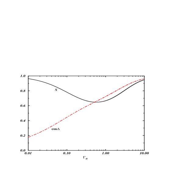
Figure 1: The power fraction $S$ of the isocurvature perturbations, and the cross-correlation $\cos\Delta$ between $\delta^{\rm ad}$ and $\delta^{\rm en}$ as a function of parameter $\Gamma_{H}$ at the end of thermal dissipative inflation for initial conditions (42) - (44).

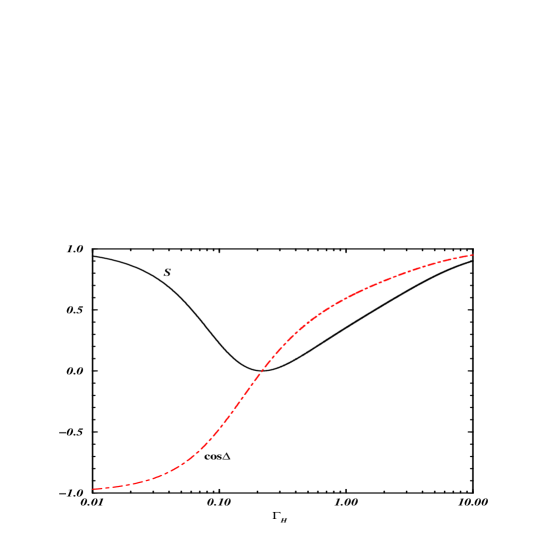
Figure 2: Same as Fig. 1 with initial conditions (48) - (50), i.e. taking into account the correlation given by the energy exchange between the background components.

V Conclusions and Discussions

We show that the thermal dissipative inflation produces the initial hybrid perturbations with significant correlation. This is largely due to the coexistence of two components, the radiation and the $\phi$ field, during the inflationary epoch. The evolution of the density perturbation of radiation and that of the $\phi$ field on scales larger than horizon are governed by different equations (D3) and (D7). Consequently after reentering the horizon, the density perturbation of radiation and that originated from $\phi$ field generally are different. The super-horizon analysis is essential to reveral the formation of the hybrid perturbations.

We have calculated the power fraction of the isocurvature perturbations ($S$), and the correlation between the adiabatic and the isocurvature perturbations ($\cos\Delta$) at the end of the inflationary epoch. Since the transition from the inflationary era to the radiation-dominated period is smooth without an intervening reheating process, the values of $S$ and $\cos\Delta$ can be directly used as the initial conditions for the radiation regime.

We found that, for each $k$-mode, $S$ and $\cos\Delta$ are mainly determined by the parameter $\Gamma_{H}$ at the instant as the perturbation mode crosses outside the Hubble horizon. That is, $S$ and $\cos\Delta$ depends entirely upon the dissipation of the inflaton. When taking into account the effect of energy exchange, $\cos\Delta$ is more sensitive to the dissipation parameter $\Gamma_{H}$. For strong dissipation cases where $\Gamma>0.217H$ the adiabatic and the isocurvature perturbations are in phase. Under weak dissipation $\Gamma<0.217H$, however, the two perturbation components are anti-correlated.

Given that the current observational constraints on $S$ and $\cos\Delta$ are rather diversepei ; val ; cro , we do not make the detail parameter fitting in this paper, but disscuss some properties of the hybrid perturbations which are useful for further model testing. Apparently, in this thermal dissipative model $S$ and $\cos\Delta$ are not independent of each other. The predicted $S$-$\cos\Delta$ relations can directly be seen from Figs. 1 and 2. These relations hold for all $k$-modes, but they are not associated with the parameter $\Gamma$. On large scales these predictions can be confronted with the CMB observation without considering the effects of evolution of perturbation during the radiation era. The relation $\cos\Delta\simeq\pm\sqrt{S}$ shown in Fig. 2 can then be tested by the observed adiabatic/isocurvature ratio and correlation. For instance, to realize the thermal dissipative inflation, the dissipation parameter $\Gamma_{H}$ can be taken in the range $\simeq 0.13-0.4$ bf ; lf1 ; lf2 . Consequently, $S$ amounts to about 10% and $\cos\Delta\simeq-0.3$ to +0.3.

Secondly, the $k$-dependence of $\cos\Delta$ in this model is governed by the $k$-dependence of $\Gamma_{H}$. On the other hand, Eqs. (42)-(43) or (48)-(49) shows that the two differences

$$\frac{d\ln\langle(\delta^{\rm ad})^{2}\rangle}{d\ln k}-\frac{d\ln\langle(\delta^{\rm en})^{2}\rangle}{d\ln k}\hskip 28.45274pt{\rm and}\hskip 28.45274pt\frac{d^{2}\ln\langle(\delta^{\rm ad})^{2}\rangle}{d\ln k^{2}}-\frac{d^{2}\ln\langle(\delta^{\rm en})^{2}\rangle}{d\ln k^{2}}$$

are also specified by the $k$-dependence of $\Gamma_{H}$. Therefore, the difference between the spectral indices, or the running spectral index, of the adiabatic and the isocurvature perturbations should also be determined by the $k$-dependence of the correlation $\cos\Delta$. For instance, if $\cos\Delta$ are $k$-independent for some range of $k$, the spectral indices should be fixed without any changes in that range. On the contrary, if there exists difference between the spectral indices of the two perturbation components, we should see a $k$-dependent $\cos\Delta$. This property is a robust prediction regardless of the initial conditions [Eqs. (42)-(44) or (48)-(50)] in use, and is effective to testing the thermal dissipative inflation model.

Appendix A Perturbation variables

Appendixes A - D will give all formulas needed for a full relativistic theory of linear perturbations for a system consisting of a $\phi$ field and a fluid, such as radiation. Most material is taken from b88 ; h123 .

A.1 Perturbing the space-time metric

The perturbed metric with respect to $\bar{g}_{ab}$ [Eq.(3)] is $g_{ab}=\bar{g}_{ab}+\delta g_{ab}$. In this paper, we are interested only in the scalar-type perturbations. For this purpose, the perturbations can be described by four variablesb88

$${\rm lapse\ function\ \alpha:} g_{00}=-a^{2}(1+2\alpha)$$ (55)

$${\rm 3-space\ curvature\ \varphi:} {\cal R}=\frac{4k^{2}}{a^{2}}\varphi$$ (56)

$${\rm expansion\ scalar\ \kappa:} \theta=3H-\kappa$$ (57)

$${\rm shear\ \chi:} \ \ \sigma_{\alpha\beta}=\chi_{\left.\right|\alpha\beta}-\frac{1}{3}g^{(3)}_{\alpha\beta}\chi^{\left.\right|\gamma}_{~{}\left.\right|\gamma}$$ (58)

where the comoving spatial metric tensor $g^{(3)}_{\alpha\beta}$ is defined by $\bar{g}_{\alpha\beta}=a^{2}g^{(3)}_{\alpha\beta}$. The vertical bar indicates a covariant derivative based on $g^{(3)}_{ab}$.

A.2 Perturbing the scalar $\phi$ field

From Eq.(5), the linearly perturbed energy density is

$$\delta\rho_{(\phi)}=\frac{1}{2}\delta(\phi,_{a}u^{a})^{2}+V^{\prime}\delta\phi.$$ (59)

The first term on the r.h.s. of (A5) can be calculated by

$$\delta(\phi,_{a}u^{a})=\delta\phi,_{a}u^{a}+\phi,_{a}\delta u^{a}=\delta\phi,_{0}u^{0}+\phi,_{0}u^{0}\left(\frac{\delta u^{0}}{u^{0}}\right).$$ (60)

By means of (A1), we have $\delta u^{0}/u^{0}\simeq-\delta g_{00}/2g_{00}=-\alpha$. Therefore, (A6) yields

$$\delta(\phi,_{a}u^{a})=\delta\dot{\phi}-\dot{\phi}\alpha.$$ (61)

Thus, (A5) becomes

$$\delta\rho_{(\phi)}=\dot{\phi}\delta\dot{\phi}-\dot{\phi}^{2}\alpha+V,_{\phi}\delta\phi.$$ (62)

Similarly, the perturbation in the pressure of the $\phi$ field is

$$\delta p_{(\phi)}=\dot{\phi}\delta\dot{\phi}-\dot{\phi}^{2}\alpha-V,_{\phi}\delta\phi.$$ (63)

For the background solution, $q_{(\psi)a}=0$. Since $q_{(\psi)a}u^{a}=0$, the linearly perturbed $q_{(\psi)a}=-\phi,_{c}u^{c}h^{b}_{a}\phi_{,b}$ can be described by

$$\delta q_{(\psi)\alpha}=\psi_{(\phi),\alpha},$$ (64)

where

$$\psi_{(\phi)}=-\dot{\phi}\delta\phi.$$ (65)

Since $\pi_{(\phi)ab}=0$ [Eq. (5)], the perturbed anisotropic pressure $\delta\pi_{(\phi),ab}=0$.

A.3 Perturbing the thermal bath

From Eq. (6), the perturbed variables of the thermal bath are given by

$${\rm perturbation\ of\ the\ energy\ density:} \varepsilon_{(r)}\equiv\delta\rho_{(r)}\$$ (66)

$${\rm perturbation\ of\ isotropic\ pressure:} \ \delta p_{(r)}=\frac{1}{3}\delta\rho_{(r)}=\frac{1}{3}\varepsilon_{(r)}$$ (67)

$${\rm energy\ flux:} \delta q_{(r)a}=\psi_{(r),\alpha}$$ (68)

$${\rm anisotropic\ pressure:} \ \ \delta\pi_{(r)ab}=0.$$ (69)

where $\psi_{(r),\alpha}$ is the energy density flux of radiation.

A.4 Perturbing the interaction terms

Using Eqs. (13) and (A6) the perturbed temporal component of the interaction term is

$$\delta Q_{(\phi)}=-\delta Q_{(r)}=-\Gamma\delta(\phi,_{a}u^{a})^{2}=2\Gamma(\dot{\phi}\delta\dot{\phi}-\dot{\phi}^{2}\alpha).$$ (70)

Similarly, the perturbed spatial component can be described by

$$\delta J_{(\phi)}=-\delta J_{(r)}=\Gamma\dot{\phi}\delta\phi.$$ (71)

Appendix B Equations of perturbation variables

Based on the perturbed variables given in §A, the evolution of these variables is governed by the following equations:

Definition of $\kappa$

$$\kappa=-3\dot{\varphi}+3H\alpha+\frac{k^{2}}{a^{2}}\chi,$$ (72)

ADM energy constraint

$$H\kappa-\frac{k^{2}}{a^{2}}\varphi=-4\pi G\left(\varepsilon_{(r)}+\dot{\phi}\delta\dot{\phi}-\dot{\phi}^{2}\alpha+V,_{\phi}\delta\phi\right),$$ (73)

momentum constraint

$$\kappa-\frac{k^{2}}{a^{2}}\chi=12\pi G\left(\psi_{(r)}-\dot{\phi}\delta\phi\right),$$ (74)

ADM propagation

$$\dot{\chi}+H\chi=\alpha+\varphi,$$ (75)

Raychaudhuri equation

$$\dot{\kappa}+2H\kappa=\left(\frac{k^{2}}{a^{2}}-3\dot{H}\right)\alpha+4\pi G\left[2\varepsilon_{(r)}+4\dot{\phi}\delta\dot{\phi}-4\dot{\phi}^{2}\alpha-2V,_{\phi}\delta\phi\right],$$ (76)

energy conservation of radiation

$$\dot{\varepsilon}_{(r)}+4H\varepsilon_{(r)}=\frac{k^{2}}{a^{2}}\psi_{(r)}+(4/3)\rho_{(r)}(\kappa-3H\alpha)+2\Gamma\dot{\phi}\delta\dot{\phi}-\Gamma\dot{\phi}^{2}\alpha,$$ (77)

momentum conservation of radiation

$$\dot{\psi}_{(r)}+3H\psi_{(r)}=-(4/3)\rho_{(r)}\alpha-(1/3)\varepsilon_{(r)}-\Gamma\dot{\phi}\delta\phi,$$ (78)

energy conservation of scalar field

$$\delta\ddot{\phi}+(3H+\Gamma)\delta\dot{\phi}+\left(\frac{k^{2}}{a^{2}}+V^{\prime\prime}\right)\delta\phi=\dot{\phi}(\kappa+\dot{\alpha})-\left[(3H+\Gamma)\dot{\phi}+2V^{\prime}\right]\alpha,$$ (79)

The momentum conservation of scalar field yields an identity.

Appendix C Gauge invariant variables

Considering a gauge transformation $\widetilde{x}^{a}=x^{a}+\xi^{a}$, in which $\xi^{a}$ is an infinitesimal quantity, any tensor quantity ${\bf T}$ transforms as $\widetilde{{\bf T}}={\bf T}-\cal L_{\xi}\it{\bf T}$, where $\cal L_{\xi}\it{\bf T}$ is the Lie derivative of ${\bf T}$ in the 4-vector field $\xi^{a}$. We may split the tensor ${\bf T}$ into its background and perturbed values; i.e., ${\bf T}=\overline{{\bf T}}+\delta{\bf T}$. The transformation of the perturbed parameter becomes $\widetilde{\delta{\bf T}}=\delta{\bf T}-\cal L_{\xi}\it\overline{{\bf T}}$. Applying the transformation to the metric tensor, we have

$$\widetilde{\delta g_{ab}}-\delta g_{ab}=-\cal L_{\xi}\it\bar{g}_{ab}\equiv-(\xi_{a;b}+\xi_{b;a})=-(\bar{g}_{ac}\xi^{c}_{~{},b}+\bar{g}_{cb}\xi^{c}_{~{},a}+\bar{g}_{ab,c}\xi^{c})~{}.$$ (80)

Since the background 3-space is homogeneous and isotropic, all the perturbation variables are gauge independent under purely spatial gauge transformations. The perturbation equations presented above are also independent of the spatial gauge transformation. Under the temporal transformation factor $T_{\xi}\equiv a\xi^{0}$, the perturbed variables are given by  b88 ; h123 :

$$\widetilde{\alpha} = \alpha-\dot{T}_{\xi}~{},$$ (81)

$$\widetilde{\varphi} = \varphi-HT_{\xi}~{},$$ (82)

$$\widetilde{\chi} = \chi-T_{\xi}~{},$$ (83)

$$\widetilde{\kappa} = \kappa+\left(3\dot{H}-\frac{k^{2}}{a^{2}}\right)T_{\xi}~{},$$ (84)

$$\widetilde{\delta\rho}_{i} = \delta\rho_{i}-\dot{\rho}_{i}T_{\xi}~{},$$ (85)

$$\widetilde{\psi}_{i} = \psi_{i}+(\rho_{i}+p_{i})T_{\xi}~{}$$ (86)

$$\widetilde{\delta Q}_{i} = \delta Q_{i}-\dot{Q}_{i}T_{\xi}~{}$$ (87)

$$\widetilde{\delta J}_{i} = \delta J_{i}+Q_{i}T_{\xi}.$$ (88)

Equations (C6) to (C9) are applicable to components $(\phi)$, $(r)$ as well as the total fluids.

Based on the time-gauge transformations [Eqs. (C2)-(C9)] and Background equations of motion [Eqs. (19) and (20)], one can construct the following gauge invariant variables:

$$\zeta=\varphi+\frac{\delta\rho_{\rm tot}}{3(\rho_{\rm tot}+p_{\rm tot})}=\varphi+\frac{\delta\rho_{(\phi)}+\delta\rho_{(r)}}{3(\rho_{(\phi)}+p_{(\phi)}+\rho_{(r)}+p_{(r)})}$$ (89)

$$\zeta_{(\phi)}=\varphi+\frac{\delta\rho_{(\phi)}+\delta J_{(\phi)}}{3(\rho_{(\phi)}+p_{(\phi)})}$$ (90)

$$\zeta_{(r)}=\varphi+\frac{\delta\rho_{(r)}+\delta J_{(r)}}{3(\rho_{(r)}+p_{(r)})}.$$ (91)

$$\psi_{(\phi r)}=\frac{\psi_{(\phi)}}{\rho_{(\phi)}+p_{(\phi)}}-\frac{\psi_{(r)}}{\rho_{(r)}+p_{(r)}}$$ (92)

Appendix D Equations of linear perturbation in the UCG

Using the uniform-curvature gauge (UCG), the equations of the perturbed variables can be obtained from Eqs. (B1) to (B8) by setting up $\varphi\equiv 0$. We have

$$\alpha=\dot{\chi}+H\chi,$$ (93)

$$\kappa=3H\dot{\chi}+\left(3H^{2}+\frac{k^{2}}{a^{2}}\right)\chi~{},$$ (94)

$$\varepsilon_{(r)}=\left(\dot{\phi}^{2}-\frac{3H^{2}}{4\pi G}\right)\dot{\chi}+\left[\dot{\phi}^{2}-\frac{1}{4\pi G}\left(3H^{2}+\frac{k^{2}}{a^{2}}\right)\right]H\chi-\dot{\phi}\delta\dot{\phi}-V^{\prime}\delta\phi,$$ (95)

$$\psi_{(r)}=-\frac{H}{4\pi G}\dot{\chi}-\frac{H^{2}}{4\pi G}\chi+\dot{\phi}\delta\phi,$$ (96)

$$\dot{\varepsilon}_{(r)}=-4H\varepsilon_{(r)}+\frac{k^{2}}{a^{2}}\psi_{(r)}+\frac{4}{3}\rho_{(r)}\frac{k^{2}}{a^{2}}\chi+2\Gamma\dot{\phi}\delta\dot{\phi}-\Gamma\dot{\phi}^{2}\alpha,$$ (97)

$$\dot{\psi}_{(r)}=-3H\psi_{(r)}-\frac{4}{3}\rho_{(r)}\left(\dot{\chi}+H\chi\right)-\frac{1}{3}\varepsilon_{(r)}-\Gamma\dot{\phi}\delta\phi,$$ (98)

$$\delta\ddot{\phi} = -\left[(3H+\Gamma)-\frac{8\pi G}{3}\frac{\dot{\phi}^{2}}{H}\right]\delta\dot{\phi}-\left[\frac{k^{2}}{a^{2}}+V^{\prime\prime}+\frac{16\pi G}{3}\frac{\dot{\phi}V^{\prime}}{H}\right]\delta\phi$$ (99)

$$-\left[\frac{32\pi G}{3}V\frac{\dot{\phi}}{H}+\left(\Gamma\dot{\phi}+2V^{\prime}\right)\right]\dot{\chi}$$

$$-\left[\left(\frac{32\pi G}{3}V-\frac{2}{3}\frac{k^{2}}{a^{2}}\right)\dot{\phi}+\left(\Gamma\dot{\phi}+2V^{\prime}\right)H\right]\chi~{},$$

$$\ddot{\chi} = -\left[H+\frac{32\pi G}{3}\frac{V}{H}\right]\dot{\chi}-\left[4\pi G\left(\frac{8}{3}V-\dot{\phi}^{2}-\frac{4}{3}\rho_{(r)}\right)-\frac{2}{3}\frac{k^{2}}{a^{2}}\right]\chi$$ (100)

$$-4\pi G\left[-\frac{2}{3}\frac{\dot{\phi}}{H}\delta\dot{\phi}+\frac{4}{3}\frac{V^{\prime}}{H}\delta\phi\right],$$

From (D1)-(D4), we have

$$\chi=\frac{4\pi G}{H}\frac{a^{2}}{k^{2}}\left[3H(\psi_{(r)}+\psi_{(\phi)})-(\varepsilon_{(r)}+\delta\rho_{(\phi)})\right],$$ (101)

and

$$\dot{\chi}=-\frac{4\pi G}{H}\left(\psi_{(r)}+\psi_{(\phi)}\right)-H\chi.$$ (102)

References

- (1) C. L. Bennett, et al., astro-ph/0302207
- (2) C. L. Bennett, et al. Astrophys. J. 464, L1 (1996).
- (3) S.L. Bridle, A.M. Lewis, J. Weller & G. Efstathiou, astro-ph/0302306
- (4) Y. P. Jing and L. Z. Fang, Phys. Rev. Lett. 73, 1882, (1994); L. Z. Fang and Y. P. Jing, Mod. Phys. Lett. A11, 1531 (1996).
- (5) A. Berera, L. Z. Fang and G. Hinshaw, Phys. Rev. D57, 2207 (1998).
- (6) H.V. Peiris, et al., astro-ph/0302225
- (7) L. A. Kofman, Phys. Lett. B173, 400(1986); D. Polarski and A. A. Starobinsky, Nucl. Phys. B 385, 623 (1992); D. Polarski and A. A. Starobinsky, Phys. Rev. D 50, 6123 (1994). F. Di Marco, F. Finelli, R. Brandenberger, Phys. Rev. D67, 063512 (2003)
- (8) D. Langlois, Phys. Rev. D59, 123512, (1999); D. Wands, N. Bartolo, S. Matarrese & A. Riotto, Phys. REv. D66, 043520, (2002); L. Amendola, C. Gordon, D. Wands & M. Sasaki, Phys. Rev. Lett. 88, 211302, (2002).
- (9) A. Berera and L.Z. Fang, Phys. Rev. Lett. 74, 1912 (1995). A. Berera, Phys. Rev. Lett. D 75, 3218 (1995).
- (10) W. L. Lee and L. Z. Fang, Phys. Rev. D59, 083503 (1999).
- (11) W.L. Lee and L.Z. Fang, Class. Quant. Grav. 17, 4467, (2000)
- (12) L.M. Hall, I.G. Moss and A. Berera, astro-ph/0305015
- (13) J. Yokoyama & A.D. Linde, Phys. Rev. D60, 083509 (1999)
- (14) A. Berera, Nucl. Phys. B585, 666, (2000)
- (15) W.L. Lee and L.Z. Fang, Int. J. Mod. Phys. D6, 305 (1997)
- (16) A.N. Taylor and A. Berera, Phys. Rev. D62, 083517, (2000)
- (17) W.L. Lee, thesis, Univ. of Arizona (1999).
- (18) G. F. R. Ellis and M. Bruni, Phys. Rev. D 40, 1804 (1989); G. F. R. Ellis, M. Bruni & J.-C. Hwang, Phys. Rev. D 42, 1035 (1990).
- (19) L.D. Landau & E.M. Lifshitz, Statistical Physics (Pergamon Press, 1989)
- (20) J. M. Bardeen, in Cosmology and Particle Physics, ed. L. Z. Fang & A. Zee, (Gordon and Breach Science Publishers, 1988)
- (21) J.-C. Hwang, Astrophys. J. 375, 443 (1991); J.-C. Hwang, Astrophys. J. 415, 486 (1993); J.-C. Hwang, Astrophys. J. 427, 542 (1994).
- (22) see e.g. J. Väliviita & V. Mubonen, astro-ph/0304175
- (23) P. Crotty, J. García-Bellido, J. Lesgourgues, & A. Riazuelo, astro-ph/0306286.