The Space Density of Redshift 5.7 Ly$\alpha$  Emitters: First Constraints from a Multislit Windows Search

Abstract

We present results from a blind, spectroscopic search for redshift 5.7 Ly$\alpha$  emission-line galaxies at Keck I. Using a band-limiting filter and custom slitmask, we cover the LRIS detector with low resolution spectra in the $8100-8250\mbox{~{}\AA}$ atmospheric window which contains no bright night sky emission lines. We find nine objects with line fluxes greater than our flux limit of $6\times 10^{-18}$ ergs s^-1 cm^-2 in our $\sim 5.1$ square arcminute field. We rule out a Ly$\alpha$  identification for six of these based on the absence of the continuum break, expected at rest-1215 Å for high-z galaxies, and/or the identification of additional emission-lines in our follow-up spectra. We find that extremely metal-poor, foreground emission-line galaxies are the most difficult type of interloper to recognize. For the three remaining emission-line objects, we identify a plausible counterpart for each object in a deep V-band image of the field suggesting that none of them has a continuum break in the $i$ band. Our preliminary conclusion is that our field contains no z=5.7 Ly$\alpha$  emitters brighter than $0.6\mbox{$L^{*}_{Ly\alpha}$}$, where $\mbox{$L^{*}_{Ly\alpha}$}\ \equiv 3.26\times 10^{42}$ ergs s^-1 . Selecting a field with zero Ly$\alpha$  emitters is marginally consistent with the no-evolution hypothesis – i.e. we expected to recover 2 to 3 Ly$\alpha$  emitters assuming the Ly$\alpha$  luminosity function at redshift 5.7 is the same as it is at redshift 3. Our null result rules out a brightening of $L^{*}_{Ly\alpha}$ by more than a factor of 1.7 from redshift 3 to redshift 5.7, or, over the same redshift interval, an increase of more than a factor of 2.2 in the number density of Ly$\alpha$ emitters. The paucity of z=5.7 Ly$\alpha$  emitters raises the question of whether the Ly$\alpha$ -selected population plays a significant role in maintaining the ionization of the intergalactic medium at $z=5.7$. We find that if the escape fraction of Ly$\alpha$  radiation is less than $0.4f_{LyC}$, where $f_{LyC}$ is the escape fraction of Lyman continuum photons, then the star formation rate in the Ly$\alpha$  emitting population is high enough in the no-evolution model (our upper limit) to maintain the ionization of the IGM at z=5.7.

1 Introduction

The Epoch of Reionization likely marks a distinct change in the galaxy population in addition to a phase transition in the intergalactic medium. Sustained star formation is probably prevented by supernova feedback in the first, low mass galaxies. Completion of Reionization likely follows the formation of fairly massive galaxies that are immune to such violent feedback. The WMAP satellite has measured a large optical depth to electron scattering after cosmological recombination implying significant reionization at $z\sim 17\pm 5$ (Kogut et al. 2003; Spergel et al. 2003). Yet the most recent re-heating must have occured more recently based on the thermal history of the intergalactic medium derived from the Ly$\alpha$  forest (Wyithe & Loeb 2003). The absence of neutral regions in the intergalactic medium at $z\lower 2.0pt\hbox{$\buildrel{\scriptstyle<}\over{\scriptstyle\sim}$}\ 6$ (Becker et al. 2001; Djorgovski et al. 2001) indicates Reionization was completed by this time. The population of galaxies responsible for Reionization, however, has yet to be recognized.

Searches for $z\sim 6$ objects latch onto either the Ly$\alpha$  emission line or the Lyman continuum break. Over cosmological distances, the HI opacity of the IGM blankets the continuum from 912 Å to the Ly$\alpha$  line effectively shifting the continuum break up to 1216Å (Madau 1995). For galaxies at redshift 5 to 7, this break crosses the $r$ and $i$ bands, producing very red $r-i$ galaxy color (or, as redshift increases, $i-z$ color). Selection by very red color, i.e. r-band (or i-band) dropouts, provides many high-redshift candidates (e.g. Yan et al. 2003) but is not a sufficient selection criterion. Galactic L and T dwarf stars, as well as $z\sim 1$ galaxies with a 4000 Å continuum break, have similar red colors in these bands. Broad-band selection followed by spectroscopic follow-up for Ly$\alpha$  emission has provided some of the best statistics on high-z galaxies to date (Lehnert & Brewer 2003), but the spectroscopic follow-up required for confirmation is difficult. Indeed, to date, the highest redshift galaxies have been discovere fd in narrow-band imaging surveys for Ly$\alpha$  emission (z=6.56, Hu et al. 2002; z=6.541, 6.578, Kodaira et al. 2003). Selection by Ly$\alpha$  emission, however, is clearly not complete as only $\sim 25\%$ of starburst galaxies at $z\sim 3$ show strong Ly$\alpha$  line emission (e.g. Steidel et al. 2000; Shapley et al. 2003). Since line selection and continuum-break selection have different shortcomings, progress will likely be made by using the two techniques in parallel.

At $z\lower 2.0pt\hbox{$\buildrel{\scriptstyle>}\over{\scriptstyle\sim}$}\ 5$, a method for detecting intrinsically faint galaxies – i.e. typical galaxies rather than rare objects – in large numbers is clearly needed to characterize their number density and clustering properties. Surveys for lensed objects along cluster caustics probe extremely deep but search tiny volumes (e.g. Ellis et al. 2001). In contrast, narrowband imaging covers large areas on the sky but does not go as deep as desired. The survey described in this paper explores a technique that may allow us to probe further down the luminosity function than narrowband imaging surveys while covering more area than lensing surveys. This multi-slit windows technique minimizes the sky noise under an emission line by dispersing the light but covers significant area on the sky by stacking multiple longslits on a single mask. We describe the strategy and our pilot observations in §2 of this paper. In §3, we present our catalog of emission-line objects and discuss the line identifications. We constrain the number density and evolution of high redshift Ly$\alpha$  emitters in §4. Section 5 summarizes our main results and the utility of the multi-slit windows technique. We adopt an $\Omega_{m}=0.3$, $\Omega_{\Lambda}=0.7$, $h=0.7$ cosmological model throughout this paper.

2 Emission-Line Search

To search for Ly$\alpha$  emission line objects at redshift 5.7, we have carried out a multislit windows search at Keck I with LRIS (Oke et al. 1995) over the atmospheric window at 8200 Å. Dispersing the light with a grating maximizes the line vs sky contrast. A narrowband filter restricts the spectral bandpass to the airglow-free region illustrated in Figure 1. Because the spectra are only $\sim 100$ Å wide, we can cut multiple long-slits on a single slit-mask, thereby greatly increasing the sky area surveyed. Similar techniques have been described by Crampton and Lilly (1999) and Stockton (1999) in the atmopheric window at 9200ÅOur aim was to systematically probe the 8200 Å  window for Ly$\alpha$  emission at z=5.7 going significantly deeper in intrinsic luminosity than the Crampton & Lilly work and narrowband-imaging surveys. Two key features of our strategy were (1) near real-time spectroscopic follow-up of emission-line candidates, and (2) a quantitative analysis of our selection function based on simulations of our detection efficiency.

2.1 Experimental Technique

The shape of the filter transmission profile is an important aspect of the experimental design. To optimally use the detector area, the filter transmission curve should have a top-hat profile with width less than or equal to that of the atmospheric bandpass. Figure 1 shows the filter transmission curve of NB8185 which Esther Hu kindly loaned to us. The transmission profile is centered at 8197 Å and has a full width at half maximum intensity (FWHM) of 106 Å and full width at 10% transmissivity of 145 Å. The filter wings transmit bright sky lines, so we spaced the spectra 165 Å apart to avoid contaminating the targetted bandpass with sky lines from neighboring slits. The increased slit spacing, over that allowed by a perfect top-hat transmission profile, effectively reduces the survey area by a factor of 1.56.

We designed our mask for the Keck I LRIS instrument and the NB8185 filter. Our selection of the 150 ${\rm mm}^{-1}$ grating (4.7  Å pix^-1) reflects a tradeoff between maximum sensitivity (somewhat higher spectral resolution) and survey volume (more slits at lower resolution). Rest-frame line widths of redshift 5.7 Ly$\alpha$  emitters are 260 km s^-1  (Bunker et al. 2003) to 340 km s^-1  (Ajiki et al. 2002), so the ideal spectral reslution for our experiment is 7 to 10  Å. We chose a slit width of 1$\farcs$5 which projects to 4.7 pixels and yields a spectral resolution of about 22 Å for a source filling the slit. At this dispersion, we fit thirty-three slitlets onto the mask at 165 Å spacing. Figure 2 shows the mask layout. Each of the longslits projects onto the full 7$\farcm$27 length of the Tektronix $2048\times 2048$ CCD. The combined slitlets subtend 5.09 square arcminutes on the sky. Stability bars prevent the thin aluminum mask from buckling; and small holes allow accurate positioning of the mask using foreground stars. The mask design does not cover the full LRIS field due to vignetting in the spectrograph, and the spectra cover just over 50% of the detector width in the dispersion direction.

The effective search area for faint objects, however, is significantly lower than the area subtended by the slits. Partial occultation by the mask renders objects with fluxes near the limiting flux of the survey too faint to detect unless they land in the center of a slit. These slit losses are derived quantitatively in §2.3. The depth of our search along the sightline, set by the filter bandpass, also has a slight dependence on flux since we measure the product $FT(\lambda)$ where $F$ is the line flux and $T(\lambda)$ is the filter transmission at the wavelength of the line. We include this effect in our modeling of the source counts. The sky noise (and therefore our sensitivity) was found to be fairly uniform across a bandpass equal to one filter FWHM. For a 1$\farcs$5 (or 1$\farcs$0) effective slit width, our survey volume is 1100 (or 730) Mpc³.

We choose a field centered at RA = 0:26:35.86, DEC = 17:11:35.15, J2000.0 This field covers the core of the rich cluster CL0024+16, redshift 0.397 (Czoske 2001). The field was chosen because it could be observed at a low airmass from Hawaii, the reddening is low $E_{B-V}=0.057$ (Schlegel, Finkbeiner, & Davis 1998), and deep broadband imaging had been obtained previously for the galaxy cluster. By selecting a cluster field, we also improve the chances of serendipitously finding a lensed object.

2.2 Observations

We obtained the search spectra 2002 November 6 with the Low-Resolution Imaging Spectrometer (Oke et al. 1995) on Keck I. A total of 21,600 s of integration time was obtained under clear skies. A series of exposures were made to allow us to track flexure, remove cosmic rays, and apply a 4″ dither along the slits. Mask alignment was verified on alternating exposures by checking the flux of the alignment stars. The median seeing measured from the spatial profiles of the alignment stars was 0$\farcs$8.

Calibration followed standard procedures using IRAF. The mean bias level of each frame was measured for each amplifier and subtracted from the detector section read by that amplifier. Pixel-to-pixel variations in gain were flattened by dividing each data frame by an appropriately normalized exposure of a quartz lamp. The images were aligned using integer shifts to compensate for instrument flexure and dithering. The 12 frames were averaged using cosmic ray rejection. The dispersion and spectral coverage were verified using Ar lines in an exposure of a calibration lamp. At such low resolution, it was not possible to directly measure the spectral resolution as all lines are blends.

We derived the flux calibration from observations of spectrophotometric standards made with a 1$\farcs$5 wide longslit. Despite the presence of an atmospheric absorption band in the filter bandpass, the two stars we observed, Feige 34 and Hiltner 600 (Massey & Gronwall 1990), gave remarkably consistent values for the sensitivity (within a few percent). The systematic errors introduced by the unknown location of a source within the slit are much larger and are discussed later in this paper. During the portion of the night with no moon, the measured sky brightness in our bandpass was $3.7\times 10^{-18}$ ergs s^-1 cm^-2 Å^-1.

Cleaning the image with sky and continuum subtraction was necessary to make automated searching possible. Although the brightest atmospheric emission lines have been blocked out of our spectra, we subtracted local sky in the combined spectral image by using a running sky window that subtended a region from 1$\farcs$06 to 3$\farcs$20 in both directions along the spatial axis. The resulting S/N in the sky subtracted frame reaches the theoretical limit set by the shot noise from sky photons, so the amplitude of the random noise fluctuations varies with wavelength as the square root of the intensity of the sky spectrum. We fit the continuum line by line for each panel of the sky-subtracted image and subtracted the fit. Emission-lines can be picked out of this cleaned image in a manner similar to object detection in direct images.

2.3 Simulations

We used simulations to gauge the sensitivity of our emission line search. We inserted artificial emission lines into our stacked and cosmic-ray cleaned – but yet not sky- or continuum-subtracted – data frames. We used artificial emission lines with Gaussian spatial and spectral profiles. The three combinations of parameters were: (FWHM_spatial, FWHM_λ) = (0.85″, 18.4Å), (1.07″, 23Å), and (1.28″, 30Å). These choices were motivated by the expected velocity dispersion – rest-frame $220$ km s^-1  FWHM (observed line width of 6 Å) and our spectral resolution – 22 Å for an object filling the slit. Since more compact objects are easier to detect, these cases include the limit of an unresolved source but also explore the sensitivity to source profile. For each line shape, we ran simulations for a range of line brightnesses from 75 to 1000 digital units (which corresponds to $2.91\times 10^{-18}{\rm~{}to~{}}3.89\times 10^{-17}$ ergs s^-1 cm^-2 for no slit loses). We avoided placing artificial emission lines on bright continuum objects, just as we avoided regions around such objects in our automated search.

We automated the recovery of these artificial sources by tuning the parameters in the SExtractor software (Bertin & Arnouts 1996). We choose regions with at least 4 connected pixels with S/N exceeding 0.5 times the rms background fluctuations. The noise level was computed in a ring around a candidate, so it sampled both the sky and continuum noise. This approach proved more robust than the human eye which may be drawn to regions of high shot noise where bright sky lines intersect continuum sources. The sky aperture underestimates the noise in regions near the edges of the bandpass, where the sky rms was higher due to the presence of airglow lines, so we excluded these regions from the automated search. The fraction of artificial emission line objects recovered determines the completeness of our emission line search. For the $0\farcs 8$ FWHM, 18.4Å FWHM sources, SExtractor finds nearly all lines brighter than $\sim$160 DN, or equivalently, to an emission line strength of $6\times 10^{-18}$ ergs s^-1 cm^-2 for a source in the center of a slit. Our results are summarized in Figure 3 which shows the completeness is higher for more compact lines.

Because of slit losses, the position of an object within the slit affects its observed flux and hence impacts our ability to detect it. Consequently, the effective area of our survey depends on the intrinsic flux of the object: the faintest objects can only be detected if they fall near the slit centre while intrinsically brighter objects can be detected closer to the slit edge and hence over a larger area. Figure 4 shows how the effective area of our survey grows as the flux of the target increases. This plot includes the small, but measured, reduction in search area caused by bright foreground objects that fall on a slit. The fluxes of sources that are only detectable exactly in the slit center – where the survey area tends to zero – are $4.5\times 10^{-18}$ ergs s^-1 cm^-2, $6.2\times 10^{-18}$ ergs s^-1 cm^-2, and $8.0\times 10^{-18}$ ergs s^-1 cm^-2 for our three fiducial object sizes. For objects that fall in the central two-thirds of a slit (i.e. 1$\farcs$0), the area searched is 3.3895 square arcminutes and the flux limit is $6\times 10^{-18}$ ergs s^-1 cm^-2, $8\times 10^{-18}$ ergs s^-1 cm^-2, and $10\times 10^{-18}$ ergs s^-1 cm^-2. In Section 4 we will use the flux-dependent survey area function shown in Figure 4 to predict expected source counts.

3 Object Identification

The dividing line between faint sources and noise fluctuations becomes increasingly fuzzy as line flux decreases. Based on the analysis of our simulations (see §2.3), we believe most lines with 160 counts or more are real detections. To ensure that we did not miss objects, we ran SExtractor (Bertin & Arnouts 1996) with the same detection criteria which were applied to the simulations in § 2.3 and identified emission lines objectively. Figure 5 shows the nine objects we found in the discovery spectra above this count limit.

We extracted spectra for the nine emission-line objects, and Table 1 summarizes their measured line properties. Notice that several line sources – B5, B4b, A21, and C28 in in order of increasing flux – have line fluxes that if at z=5.7 would imply Ly$\alpha$  luminosities similar to $L^{*}_{Ly\alpha}$, where $\mbox{$L^{*}_{Ly\alpha}$}\equiv 3.26\times 10^{42}$ ergs s^-1 . We adopt this fiducial luminosity for the knee of the luminosity function based on the typical Ly$\alpha$  luminosities measured at z=3 (Steidel et al. 2000) and at z= 4.9 (Ouchi 2003). If $L^{*}_{Ly\alpha}$ does not evolve, an $L^{*}_{Ly\alpha}$ emitter at z=5.7 has an observed flux of $1.09\times 10^{-17}$ ergs s^-1 cm^-2. Our faintest emission line source, B5, would have a line luminosity of $0.77\mbox{$L^{*}$}$ if it were at $z=5.7$. For completeness, we remind the reader that we do not know where in the slit a particular source fell so the line fluxes are technically lower limits.

Any viable high-redshift Ly$\alpha$  emitter will have at least a factor of 5 to 10 continuum break just blueward of the Ly$\alpha$  line due to attenuation from intergalactic gas (Madau 1995). Figure 5 reveals relatively bright continuum emission to both sides of the line in B5, D21b, and D22. We reject these three objects as Ly$\alpha$  candidates on the basis of the absence of a continuum break; and we tentatively identify D22 as a blend of H$\alpha$  and [NII] 6584 on the basis of the line shape.

For the other galaxies, the follow-up observations described in the next section were required to determine their identity, but we draw attention to a few interesting attributes derived from the discovery spectra first. For example, extremely high equivalent widths are often more easily fitted by the Ly$\alpha$  line than any other emission line, and we find C17 and D21 have extreme equivalent widths. Specifically, using the continuum blueward of the C17 line, we measure observed equivalent width of 490 Å. No continuum is detected near D21, and we find the equivalent width must exceed 500 Å. In addition to their high equivalent widths, objects C17 and D21 are the only two candidates not spatially resolved in 0$\farcs$8 seeing.

3.1 Follow-Up of Emission-Line Candidates

3.1.1 Follow-Up Spectroscopy

To ensure accurate alignment of our follow-up mask on the desired targets, we milled the follow-up mask using a modified version of the mask design file from our search mask. Consequently, the relative positions of set-up star boxes and those slit segments that contained the five candidates of interest were preserved, allowing us to position our follow-up mask’s slits exactly on the same place in the sky as those in our search mask. To allow us to use higher dispersion and broader spectral coverage for the follow-up observations without generating overlapping spectra, slit segments containing no Ly$\alpha$  candidates were removed from the mill file. This procedure allowed us to be confident that our targets were indeed in the slits of our follow-up mask.

We obtained follow-up spectra of emission-line objects A21, B4b, B5, D11, and D21 on 2002 November 9 with LRIS. We inserted the 831 ${\rm mm}^{-1}$ grating blazed at 8200Å to improve the spectral resolution on the red side (0.93Å pix^-1). Blue light diverted by the D680 dichroic was dispersed by a 300 mm^-1 grism blazed at 5000 Å. We removed the narrowband filter to increase the spectral coverage from $\sim\lambda 6800$ to the atmospheric limit at $\sim\lambda 3200$ in the blue and $\lambda 6800$ to $\lambda 8700$ in the red.

Five hours of integration time were obtained under thin cirrus clouds and 0$\farcs$8 seeing fwhm. We guided in the i-band to keep the $\sim\lambda 8200$ emission centered in the slits. Since there is no atmospheric dispersion compensator on LRIS, the targets are only in the slits on the blue side for a few hours. The measured width of the night sky lines was 4.7 pixels, or 4.4 Å. The image processing steps were the same as those described in Section 2.2. Figure 6 shows the emission line sources A21, D11, and D21 were redetected in our follow-up spectra. Object B4b was not re-detected.

3.1.2 Imaging Follow-Up

We mapped the positions of the emission line candidates onto a direct image of the sky taken with LRIS. Since we do not know the position of an object within the slit, the error perpendicular to the slit direction is $\pm 0\farcs 75$. We computed only the lowest order term for the coordinate transformation along the slit, and the average error for a set of bright, test objects was $0\farcs 55$. The coordinates on the LRIS image were tied to a deep V-band image of CL0024V (Czoske et al. 2001). None of our emission line candidates were near bright stars or galaxies. Object D21 lies along a set of arclets near the cluster although the spectral follow-up identified the line as H$\alpha$  emission from a foreground galaxy. Although our spectroscopic analysis yielded 3 emission lines which could be Ly$\alpha$  at z=5.7, we find a faint V-band object within 2$\farcs$0 of the position of each. The small size of these galaxies is consistent with either irregular galaxies at $z\sim 0.6$ or dwarf irregular galaxies at $z\sim 0.24$ The faintest counterpart, related to C28, consists of two small clumps. The brightest counterpart, related to B4b, appears to be a spiral galaxy near, but not on, the slit. Deep $i$ or $z$ imaging of these fields would determine whether there is another object closer to our predicted position. Follow-up spectroscopy of each V-band counterpart would also quickly determine if it is the emission-line source.

3.2 Conclusions on Line Identifications

We draw the following conclusions about the identity of the emission-line objects in Table 1.

• A21: Several emission lines were detected in the follow-up spectrum. We identify the discovery line as [OIII] $\lambda 5007$; and the emitter is at $z=0.656$. See Figure 6.

• B4b: Emission-line source not detected on follow-up mask.

• B5: Lack of a continuum break across the emission line rules out Ly$\alpha$  identification.

• C17: If the emitter is at z=5.7, the line luminosity is brighter (and more rare) than the objects expected in our survey volume. We tentatively identify a V band counterpart for this object which, if correct, indicates the object is not at high redshift. We cannot rule out a Ly$\alpha$  identification at this time however.

• C28: Marginal continuum detection to both sides of the line leads us to suspect this object is not Ly$\alpha$ . Continuum detection is too weak to rule out a Ly$\alpha$  identification however.

• D11: Several emission lines were detected in follow-up spectrum. We identify the discovery line as [OIII] $\lambda 5007$ at $z=0.662$. See Figure 6.

• D21: This object lies near the cluster caustic. No continuum or line emission, aside from the single line at $\lambda 8189.65$, was detected from D21 in the red follow-up spectrum ($\lambda 7080-\lambda 8970$). The line profile has a Gaussian FWHM of 3.7 Å which rules out an identification as [OII] 3726, 29 at z=1.2. However, a series of emission lines identified as [OIII] 4959, 5007, [OIII] 4364, and the Balmer series are seen in the blue spectrum. The high equivalent width line originally detected turns out to be H$\alpha$ emission at z=0.248. The 3-sigma upper limit on the [NII] 6583 line, which is not detected, is $<1\%$ of the strength of the H$\alpha$ line. Our red spectrum covered [ArIII] 7135, HeI 6678, [SII] 6731, [NII] 6583, [OI] 6300, and He 5578. None of metal lines are strong in this obviously very metal poor galaxy; and the He I lines fell on strong night sky lines.

• D21b: Strong continuum emission, but lack of continuum break rules out Ly$\alpha$  identification.

• D22: Strong continuum detected, but lack of continuum break rules out Ly$\alpha$  identification. Second line redward of brightest line presents correct offset for H$\alpha$ and [NII] 6583 at a redshift $z\sim 0.24$.

Objects B4b, C17, and C28 are our only objects for which a Ly$\alpha$  identification is plausible. Within the positional uncertainties, the position of each of these emission-line sources matches the location of an object detected in a deep V-band image. In summary, we urge caution in the use of single-line redshifts for high-redshift galaxies. Many of the faint emission-line objects that we found turn out to be foreground galaxies upon more detailed inspection. Our sample contains at most three Ly$\alpha$  emitters brighter than $7.8\times 10^{-18}$ ergs s^-1 cm^-2, and none of these three candidates appears likely to be a genuine z=5.7 galaxy

4 Discussion

Since our survey sensitivity and search volume are well understood from simulations, our observations constrain the properties of the z=5.7 population of Ly$\alpha$ emitters. The clean detection of objects B5 and C28 confirm that a Ly$\alpha$   emission line with $L^{*}$ luminosity would easily be detected, and we are confident that galaxies as faint as 0.6$L^{*}$ would be detected $>85\%$ of the time. The paucity of Ly$\alpha$  emitters found excludes a high density of bright galaxies with high Ly$\alpha$  escape fractions. We quantify this statement in §4.1 and §4.2. In §4.3, we discuss whether bright, Ly$\alpha$  selected galaxies can maintain the ionization of the intergalactic medium at z=5.7.

4.1 Density of Ly$\alpha$  Emitters

To gain some insight into the properties of the high-redshift galaxy population, we parameterize the Ly$\alpha$  emitting population by a Schecter luminosity function $\phi(L/\mbox{$L^{*}$})d(L/\mbox{$L^{*}$})=\phi^{*}(L/\mbox{$L^{*}$})^{\alpha}e^{-L/L^{*}}d(L/L^{*})$, where the three parameters $\phi^{*}$, $L^{*}$, and $\alpha$ describe the number density, Ly$\alpha$  luminosity of the bright-end turnover, and the faint-end slope. We expect our survey to find

$$N=\int_{L_{min}}^{L_{max}}\phi(L/\mbox{$L^{*}$})V(L/\mbox{$L^{*}$})\xi(L/\mbox{$L^{*}$})d(L/\mbox{$L^{*}$})$$ (1)

galaxies. The survey volume, $V$, and the survey completeness, $\xi$, depend on luminosity because the survey area and bandwidth decrease as the line flux approaches the limiting flux of the survey (see §2.3). We compute $V(L/\mbox{$L^{*}$})$ from the cosmological volume increment per unit redshift, the accessible redshift interval (from Figure 1), and the effective survey area (from Figure 4). Figure 3 illustrates the completeness function, $\xi(L/\mbox{$L^{*}$})$. Guided by the properties of the Ly$\alpha$  population at redshifts 3 and 4 (Steidel et al. 2000; Ouchi et al. 2003), we adopt the following luminosity function – $\phi^{*}=0.0055$ Mpc^-3, $\mbox{$L^{*}$}=3.26\times 10^{42}$ ergs s^-1 , and $\alpha=-1.2$ (-1.6) – and integrate down to the limiting flux of the survey. For the no-evolution scenario, we predict our survey should return 2.5 (2.4) Ly$\alpha$  emitters per field on average.

Using the above formalism, we test the hypothesis that the luminosity function does not evolve between redshift 3 and 5.7. Suppose we observe many fields, we would expect to recover the mean – i.e. 2 to 3 Ly$\alpha$  emitters – on average. Assuming (for the moment) the galaxies are randomly distributed in space (i.e. Poisson statistics), the probability of obtaining 0 (or 1) object is 8.2% (20%). The paucity of Ly$\alpha$  emitters found in our field is therefore marginally consistent with no-evolution in the Ly$\alpha$  emitting galaxy population between redshift 3 and 5.7.

It is interesting to consider how strong lensing by the cluster CL0024+16 might affect the results of our survey. Galaxies seen through the cluster core will typically be magnified by a factor $\sim 2$. The cluster core subtends $\sim 18\%$ of the area covered by our mask, so we would expect 1 in 5 background galaxies to be lensed by a factor of two. We find no statistically significant clustering among the emission-line objects in our field. Only two of our emission line objects clearly have redshifts greater than the cluster redshift, and one of these, A21, is projected well beyond the cluster core. Given that we find no high redshift galaxies, accounting for the presence of a lensing cluster in our field would strengthen our claim that the emission line galaxy population does not undergo positive evolution from redshift 3 to redshift 5.7. Stronger magnification is only possible near the caustics where our mask subtends an insignificant area.

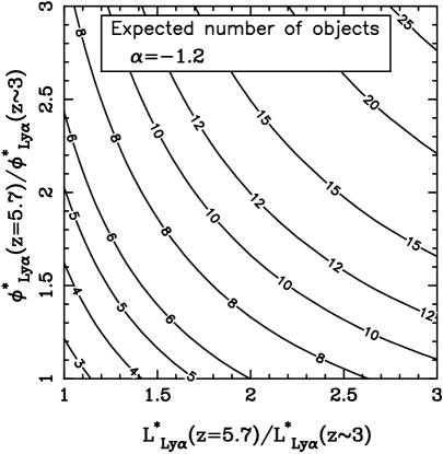
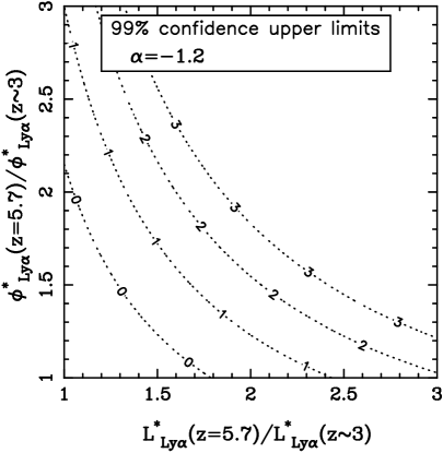
Figure 7: (a) Predicted survey yield for various evolution models of the Ly$\alpha$  luminosity function. The axes indicate the amount of evolution in the number density (vertical axis) or luminosity density (horizontal axis) relative to our baseline luminosity function ( $\mbox{$L^{*}_{Ly\alpha}$}(z=3)\equiv 3.26\times 10^{42}$ ergs s^-1, $\phi^{*}_{Ly\alpha}(z=3)=0.0055$ Mpc^-3). The faint end slope of $\alpha$=-1.2 was assumed for the luminosity function, but the results do not depend significantly on the assumed $\alpha$. For a Ly$\alpha$ luminosity function that does not evolve between $z$$\sim$$3$ and $z$=5.7, we expect to recover $\sim$2.5 $z$=5.7 Ly$\alpha$ emitters on average. (b)Constraints on the evolution of the Ly$\alpha$ luminosity function from $z$$\sim$3 to $z$=5.7. The leftmost curve — labelled “0” — shows the upper limit (Poisson 99% confidence) on the amount of luminosity and density evolution in the Ly$\alpha$ luminosity function allowed by the null result of our survey. The area of parameter space to the right of the curve is ruled out by our lack of Ly$\alpha$ detections. The other curves show the upper limits had we detected 1, 2, or 3 Ly$\alpha$ emitters. Evidently between redshift 3 and 6, $L^{*}_{Ly\alpha}$ does not brighten by more than a factor of 1.8 and $\phi^{*}_{Ly\alpha}$ does not increase by more than a factor of 2.1.

Our results place strong constraints on the evolution of the Ly$\alpha$ -emitting population. For any model of the luminosity function described by $\phi^{*}$, $L^{*}$, and $\alpha$, we can calculate the number of Ly$\alpha$ -emitters our survey would detect. Figure 7a shows the expected yield of Ly$\alpha$  emitters per field over a grid spanning a factor of three evolution in $L^{*}$ and $\phi^{*}$. For each of these models, we computed the probability of our field yielding zero Ly$\alpha$  detections. The leftmost dashed line in Figure 7b illustrates the 99% Poisson confidence contour for our null result. We find that in the limit of no density evolution, the value of $L^{*}_{Ly\alpha}$ appears unlikely to brighten by more than a factor 1.8 between z=3 and z=5.7. Similarly, in the limit of no luminosity evolution, the number density of Ly$\alpha$  emitters does not increase by more than a factor of 2.1 between z=3 and z=6. The number of predicted objects is not sensitive to the faint-end slope of the luminosity function because our observations reach only 0.6$L^{*}$. The other curves show the upper limits had we detected 1, 2, or 3 Ly$\alpha$  emitters. Even if a similar observation of another field yielded 2 Ly$\alpha$  detections, we would conclude that between z=3 and z=6 $L^{*}$ brightens by less than a factor 3 and the comoving density of Ly$\alpha$  emitters grows by less than a factor of 3.75. Our results rule out strong positive evolution in the Ly$\alpha$ - emitting population from z=3 to z=6.

4.2 Impact of Galaxy-Galaxy Clustering on Results

The true variance in galaxy counts $N$ about the mean $\mu$ will be larger than the Poisson variance, $\delta^{2}=<(N-\mu)^{2}>=\mu$, by an amount reflecting the clustering strength, $\mu^{2}\xi(r)$ (e.g. Peebles 1993). The correlation function, $\xi(r)$, has not yet been measured for high-redshift Ly$\alpha$  emitters, but we can illustrate how much clustering would be required to significantly change our conclusions. If clustering reduces the number of Ly$\alpha$  emitters in our field from 2.5 to 0, then $\delta\rho/\bar{\rho}=1$ and $\xi(r)=1$. The variance of the counts increases to $\delta=\sqrt{\mu+\mu^{2}\xi(r)}=2.0$, which is not much larger than the value of $\delta=1.6$ expected for a random source distribution. Yet this estimate implies a higher degree of clustering than the Steidel et al. (1999) $\delta\rho/\bar{\rho}\approx 0.25$ estimate for Ly$\alpha$  emitters at $z\sim 3$. It seems unlikely, therefore, that clustering of Ly$\alpha$  emitters could account for the paucity of Ly$\alpha$  emitters found by our survey; and our conclusion - that $L^{*}$ Ly$\alpha$  emitters cannot increase much in luminosity or increase in number density between $z\sim 3$ and $z\sim 5.7$ – holds even if the population is fairly strongly clustered.

To place further constraints on the potential impact of clustering, it is interesting to ask whether our number density is consistent with the yield of high-redshift galaxies from other Ly$\alpha$  surveys. For a non-evolving Ly$\alpha$  population, we expected to recover only a couple Ly$\alpha$  emitters in our pilot survey, and we expected them to have sub-$L^{*}$ luminosities. Narrowband imaging surveys, in contrast, cover larger areas but recover only objects brighter than roughly 2$L^{*}$. The no-evolution model implies that a survey must, on average, cover 21 square arcminutes on the sky to return one 2.0$L^{*}$ Ly$\alpha$  emitter from a 103 Å wide bandpass at z=5.7. This area corresponds to a survey volume $\sim 4500$ Mpc³. The LALA group has three secure identifications of $z=5.7$ Ly$\alpha$  emitters which corresponds to $2.5\times 10^{4}$ Mpc³ per 2.5$L^{*}$ Ly$\alpha$  emitter. For our adopted cosmology, the volume per emitter for the Hu et al. narrowband imaging is smaller at roughly 6900  Mpc³. The Ly$\alpha$ search at Subaru confirmed a bright $z=5.7$ emitter ($F=4.1\times 10^{-17}$ ergs s^-1 cm^-2; Taniguchi et al. 2003) after searching about $3.4\times 10^{4}$ Mpc³. Considering the uncertainties inherent in gross comparisons among these surveys, our limits on the number density of Ly$\alpha$  emitters appear to be consistent with the other results. It remains plausible then that the Ly$\alpha$  emitting population could maintain the ionization of the IGM at $z=5.7$ and be related to the population responsible for cosmic reionization.

Lehnert & Bremer (2003) selected galaxies between z=4.8 to z=5.8. using the broadband drop-out technique and spectroscopically confirmed two Ly$\alpha$  emitters in the 8200 Å atmospheric window. Their survey volume in the z=5.697 to z=5.710 window is only $\sim 9.72\times 10^{3}$ Mpc³, but both objects found are bright sources typical of those found by narrowband-selection (BDF 1:10 $F=2.45\times 10^{-17}$; BDF 2:19 $F=2.51\times 10^{-17}$). The implied number density of $L\lower 2.0pt\hbox{$\buildrel{\scriptstyle>}\over{\scriptstyle\sim}$}\ \mbox{$L^{*}$}$ Ly$\alpha$  emitters in the field is roughly 1 per 5000 Mpc³. Lehnert & Bremer (2003) conclude that their objects cannot maintain the ionization of the IGM and suggest that lower luminosity galaxies contribute to the ionization of the IGM. Since some of the emission line galaxies that we detected are too faint in the continuum to be selected by the Lehnert & Bremer survey, their result may be consistent with our conclusion. To date then, the different high redshift galaxy surveys seem to yield mutually plausible constraints on the high redshift galaxy population. Consequently, we cannot yet use the variance in Ly$\alpha$  emitting galaxies among surveys to empirically estimate their clustering properties.

4.3 Are There Enough High-Redshift Galaxies to Ionize the Intergalactic Medium?

Recent observations of high redshift quasars pin the redshift of the final reionization epoch near $z\sim 6$ (Becker et al. 2001; Djorgovski et al. 2001), so the formation rate of stars and quasars must remain high enough following the end of Reionization to at least offset the recombination rate of the intergalactic gas. The identity of the objects that maintain the ionization of the intergalactic medium at $z=5.7$ remains an open question. While quasars dominate the production of intergalactic Lyman continuum radiation by $z=0$, at $z\sim 3$ more ionizing flux escapes from Lyman-break-selected galaxies than from quasars (Madau et al. 1999; Steidel et al. al 2001). The contribution from quasars at $z\sim 5.7$ appears to fall far short of that needed to maintain IGM ionization (Fan et al. 2001). It is interesting to examine whether the bright Ly$\alpha$  emitting population is a plausible source of the required ionizing luminosity.

The time from redshift z=5.7 to the reported completion of Reionization at z=6 (Becker et al. 2001; Djorgovski et al. 2001) is only $152h_{0.7}^{-1}$ Myr. Hence the galaxy population responsible for Reionization may still be present at $z=5.7$. A hydrogen atom in the IGM consumes several ionizing photons in this short period. The recombination time at z=5.7, averaged over a clumpy IGM, is $\bar{t}_{rec}=64~{}{\rm Myr~{}}(0.041/(\Omega_{b}h_{70}^{2}))C_{30}^{-1}$, where $C_{30}$ is the ionized hydrogen clumping factor in units of $C\equiv<n_{HII}^{2}>/\bar{n}_{HII}^{2}=30$ (Madau et al. 1999). To raise the filling factor, $f_{HII}$, of ionized regions in the IGM to unity, the number of ionizing photons escaping from galaxies over the recombination timescale must equal or exceed the baryon density. Following Madau et al. (1999), the critical production rate of ionizing photons is $\dot{N}_{H}=\bar{n}_{H}(0)/\bar{t}_{rec}(z)$ per unit comoving volume, which we can write as

$$\dot{N}_{H}=10^{51.34}{\rm~{}s}^{-1}{\rm~{}Mpc}^{-3}~{}C_{30}\left(\frac{1+z}{6.7}\right)^{3}\left(\frac{\Omega_{b}h_{70}^{2}}{0.041}\right)^{2}.$$ (2)

For an initial stellar mass function $dM/dN\propto M^{-2.35}$ (i.e. Salpeter IMF), continuous star formation produces ionizing photons at a rate of $\dot{N}_{H}=10^{53.4}$ s^-1 per solar mass of 1.0${\rm~{}M_{\odot}}$ to 100${\rm~{}M_{\odot}}$stars formed in 1 year (Leitherer et al. 1999). Including the mass of 0.1 to 1.0${\rm~{}M_{\odot}}$ stars formed by this IMF, the minimum cosmic star formation rate required to keep the universe ionized at z=5.7 in the absence of any ionizing flux from quasars is

$$\dot{\rho}_{*}=0.0223\mbox{$~{}{\rm M_{\odot}}$~{}yr${}^{-1}$}{\rm Mpc}^{-3}C_{30}\left(\frac{1+z}{6.7}\right)^{3}\left(\frac{\Omega_{b}h_{70}^{2}}{0.041}\right)^{2}f_{LyC}^{-1},$$ (3)

where $f_{LyC}$ is the fraction of Lyman continuum photons escaping from galaxies. Theoretical simulations predict that the escape fraction, $f_{LyC}$, will become large when a starburst-driven wind blows out of a galactic disk (Fujita et al. 2003). In nearby starburst galaxies, measured values of $f_{LyC}$ are less than 15% (Leitherer et al. 1995; Hurwitz et al. 1997). Some high-redshift galaxies have higher escape fractions (Steidel et al. 2001), but no clear consensus about escape fractions from high-redshift starbursts has been reached (Fernández-Soto et al. 2003). Although the most appropriate value of $f_{LyC}$ for high-redshift galaxies clearly remains to be determined, values up to unity remain plausible for now.

The Ly$\alpha$  line is a notoriously poor measure of the galactic star formation rate. The large scattering cross section in the line produces a high probability that a Ly$\alpha$  photon will be absorbed by a dust grain. The effective optical depth in the line can be dramatically reduced, however, by bulk motions in the ISM which Doppler shift the line photons away from the resonance. Observations of the Ly$\alpha$  emission/absorption profile show wide variety among even starburst galaxies (Shapley et al. 2003), and models suggest the emission line flux depends as much on the evolutionary state of the starburst wind as on the absolute value of the star formation rate (SFR) (Tenorio-Tagle et al. 1999). For purposes of illustration, we simply parameterize the line luminosity in terms of the fraction of Ly$\alpha$  photons that escape the galaxy $f_{Ly\alpha}$. For a Salpeter stellar IMF extending from 0.1${\rm~{}M_{\odot}}$ to 100${\rm~{}M_{\odot}}$  a star formation rate of 1.0 $~{}{\rm M_{\odot}}$ yr^-1 yields an H$\alpha$ emission line luminosity of $1.26\times 10^{41}$ ergs s^-1 (Kennicutt 1998). Using the Case B ratio of the H recombination lines at low density (Ferland & Osterbrock 1985), we find $L_{Ly\alpha}=8.32f_{Ly\alpha}L_{H\alpha}$. Substituting for the star formation rate in Equation 3, we derive the critical (comoving) luminosity density of Ly$\alpha$  emission,

$$\L_{Ly\alpha}=2.34\times 10^{40}{\rm~{}erg~{}s}^{-1}{\rm~{}Mpc}^{-3}~{}\left(\frac{f_{Ly\alpha}}{f_{LyC}}\right)C_{30}\left(\frac{1+z}{6.7}\right)^{3}\left(\frac{\Omega_{b}h_{70}^{2}}{0.041}\right)^{2},$$ (4)

required to maintain the ionization of the IGM at z=5.7.

We may use Equation 4 to explore whether the population of z=5.7 Ly$\alpha$  emitters can make a significant contribution to the required ionizing luminosity. For our fiducial model ($\phi_{*}=0.0055$ Mpc^-3, $\mbox{$L^{*}_{Ly\alpha}$}=3.26\times 10^{42}$, and $\alpha=-1.2$), the Ly$\alpha$  luminosity produced by galaxies brighter than 0.6$L^{*}$ is $\L=0.0028\mbox{$L^{*}$}$ Mpc^-3. This population can only maintain the ionization of the IGM if $f_{Ly\alpha}$ is small (relative to $f_{LyC}$) - i.e. most of the emitted Ly$\alpha$  is absorbed and therefore not detected. Using equation 3, our limits on the number density of galaxies brighter than 0.6$L^{*}_{Ly\alpha}$  imply the escape fraction of Ly$\alpha$  photons would have to be $f_{Ly\alpha}\leq\ 0.39f_{LyC}$ if these relatively bright galaxies were to maintain the ionization of the IGM.

Since the optical depth in the Ly$\alpha$  line is much higher than the optical depth at the Lyman limit, it is possible for a large fraction of the Lyman continuum photons to escape while most Ly$\alpha$  photons are absorbed by dust after many scatterings. A Ly$\alpha$  escape fraction $f_{Ly\alpha}\sim 0.4$ also seems plausible when the properties of the known $z\sim 6$ galaxies are considered. For SSA22-HCM1 (z=5.74), Hu et al. (1999) derive a SFR from the ultraviolet continuum that is twice as large as that derived from the Ly$\alpha$  line. (Using the flux to SFR scale adopted in this paper, we get a SFR from the continuum that is six times larger than that estimated from the line flux, so a value of $f_{Ly\alpha}$ in the range of 0.2 to 0.5 is at least plausible.) If the number of luminous Ly$\alpha$  emitters at z=5.7 is similar to our inferred upper limit on their number density and the Ly$\alpha$  escape fraction $\lower 2.0pt\hbox{$\buildrel{\scriptstyle<}\over{\scriptstyle\sim}$}\ 40\%$, then relatively bright Ly$\alpha$  emitters with $L\sim\ \mbox{$L^{*}_{Ly\alpha}$}\$ can maintain the ionization of the IGM at $z=5.7$. A significant deficit of $L^{*}$ Ly$\alpha$  emitters relative to this no-evolution model would suggest that another population of galaxies, perhaps large numbers of dwarf galaxies, must be present to maintain the ionization of the IGM. That measurement should be possible soon.

Continuum-break-selected surveys also find a paucity of galaxies at high redshift. In particular, Lehnert & Bremer (2003) conclude that the bulk of the ionizing flux that reionized the universe came from faint galaxies with $M_{AB}(1700{\rm\AA})>-21$. They find a lower density of $z\sim 5.3$ r-band dropouts than expected from no-evolution predictions tied to the lyman-break-selected galaxy population at z=3 and 4. The ultraviolet luminosity density from their $z\sim 5.3$ drop-outs is considerably less than that required to ionize their survey volume. Drop-out searches complement the Ly$\alpha$  searches because the inherent biases are quite different. (The dropout technique yields some false-positive detections, but the Ly$\alpha$  surveys may miss galaxies entirely.) Constraints from both techniques will probably be required to pin down the population producing the ionizing background at $z\sim\ 6$.

5 Conclusions and Outlook

We have shown that the multi-slit windows technique provides a very sensitive means of searching for emission-line galaxies. It probes significantly larger volumes than surveys of cluster caustics but reaches sub-$L^{*}$objects which are largely inaccessible to narrow-band imaging surveys at high redshift. In our pilot survey, most of the emission-line sources were found to be foreground galaxies. It is possible that the Ly$\alpha$  emitting population at z=5.7 is described by the same $L^{*}$ and $\phi_{*}$ as the Ly$\alpha$ -emitting population at $z\sim 3$ to 4, and we recovered no Ly$\alpha$  emitters simply because the richness of our field was poor compared to an average field. However, the paucity of Ly$\alpha$  emitters in our field does strongly rule out significant positive evolution in the luminosity function. Neither the characteristic luminosity nor number density of Ly$\alpha$  emitters can increase much between z=3 and z=5.7 – a period long enough, $1.1h^{-1}_{0.7}$ Gyr, to allow several cycles of bursting activity and fading (Sawicki & Yee 1998; Shapley et al. 2001).

Since the recombination time of the intergalactic gas is shorter at higher redshift, the paucity of Ly$\alpha$  emitters at $z\sim 5.7$ raises the question of whether the Ly$\alpha$ -selected population can keep the IGM ionized at $z=5.7$. In the no-evolution scenario, in order for the inferred star formation rate to be high enough to maintain the ionization of the intergalactic medium, the fraction of Ly$\alpha$  emission escaping must be less than 40%. This average Ly$\alpha$  escape fraction does not appear to be unusual. Indeed, only 25% of starburst galaxies at z=3 have Ly$\alpha$  in emission (Shapley et al. 2003). Our constraint is strictly an upper limit, however. Additional observations will either recover Ly$\alpha$  emitters in number or push this upper limit low enough to require another population of galaxies (e.g. perhaps dwarf galaxies) to maintain ionization. The existence of another population of dwarf starbursts is suggested by the detection of a z=5.7 Ly$\alpha$  emitter with de-lensed flux of only $2\times 10^{-18}$ ergs s^-1 cm^-2 in a search volume an order of magnitude smaller than that of our survey (Ellis et al. 2001).

Future surveys with the multislit windows technique are expected to produce about a dozen high-redshift galaxies per pointing. The gains will come from a combination of improved sensitivity, the larger field of view provided by new cameras, and multi-night observing campaigns. Dispersing the spectra to a rest-frame velocity dispersion of 200 km s^-1 , which is about $\sim 5.5$ Å, will reduce the sky noise by another factor of 3 to 4. The throughput can probably be doubled by using a more efficient dispersing element. It should be possible, therefore, to reach fluxes a factor of 2.5 to 3 times fainter than our limit of $6.2\times 10^{-18}$ ergs s^-1 cm^-2 in a single night of observing time. Although the cost of higher dispersion would normally be reduced area, the new generation of large format CCD arrays more than makes up for the decrease in survey area.

Atmospheric windows at longer wavelength allow the technique to be extended to higher redshifts. However, even in the next window at 9200 Å (z = 6.5), the exposure time required to reach a given luminosity is nearly a factor of two higher than that required at z=5.7 (in the 8200 Å window). We would expect a large multislit windows survey in the 8200 Å window to yield a secure measurement of the number density of dwarf (i.e. sub $L^{*}$) Ly$\alpha$  emitters at z=5.7.

Table 1: Properties of Emission-Line Sources

Object ID	FWHM	FWHM	Line Flux	Line Flux	EWo	Line ID
(MS-0h17)	(″)	( Å)	(Counts)	($10^{-17}$ ergs s-1 cm-2)	( Å)	(redshift)
A21	1.47	18.0	$340\pm 50$	$1.30\pm 0.2$	28	[OIII], z=0.656
B4b	1.48	15.1	$290\pm 29$	$1.1\pm 0.1$	$>80$	Unlikey Ly$\alpha$  Line
B5	1.40	10.0	$220\pm 50$	$0.84\pm 0.2$	9	Not Ly$\alpha$
C17	1.10	17.2	$1200\pm 44$	$4.80\pm 0.2$	490	Unlikely Ly$\alpha$  Line
C28	1.29	19.5	$430\pm 56$	$1.7\pm 0.1$	80	Unlikely Ly$\alpha$  Line
D11	1.08	16.5	$640\pm 38$	$2.5\pm 0.2$	47	[OIII], z=0.662
D21	0.86	17.7	$6280\pm 66$	$24.4\pm 0.3$	$>500$	H$\alpha$ at z=0.248
D21b	1.38	20.8	$700\pm 90$	$2.7\pm 0.4$	32	Not Ly$\alpha$
D22	1.16	20.4	$2760\pm 110$	$10.7\pm 0.4$	40	Likely H$\alpha$ +[NII]

Table Notes –

(1) Object name on Martin & Sawicki mask for field at 0h 17^∘.

(2) Extent of emission line along the slit.

(3) Observed line width. All lines are unresolved.

(4) Counts in the emission line.

(5) Line flux derived assuming the average filter transmission over the bandpass.

(6) Emission-line equivalent width.

Figure 1: Relative intensity of the Mauna Kea night sky (courtesy of Tom Slanger). The transmission of filter NB8185 (kindly loaned by Esther Hu) illustrates the atmospheric window probed by our survey.

Figure 2: Slitmask layout for the search mask. The mask consisted of 33 longslits interrupted by three bars needed for structural rigidity. Small squares are holes for alignment stars used for positioning the mask on the sky. Dispersion direction is left to right.

Figure 3: Survey sensitivity. The fraction of simulated objects recovered by the automated detection routine for the three combinations of object size parameters. We define our completeness limit at 160 counts, which, in the absence of slit losses, corresponds to 6$\times$$10^{-18}$ erg s^-1 cm^-2.

Figure 4: Our survey area as a function of emission line flux. The horizontal line denotes the geometric angle subtended by the slitlets. Slit losses reduce the transmitted flux, and the faintest emission lines are only detected when the objects land in the center of the slit.

Figure 5: Emission-line candidates found by the automated search. The arrows denote 5${}^{\prime\prime}~{}$and 100 Å in the spatial and spectral directions respectively. Wavelength increases from left to right.

Figure 6: Follow-up spectra for objects A21, D11, and D21. None of the confirmed line identifications are Ly$\alpha$ .

References

- (1)
- (2) Ajiki, M. et al. 2002, ApJ, 576, L25
- (3)
- (4) Bertin, E. & Arnouts, S. 1996, A&AS, 117, 393
- (5)
- (6) Becker, R. H. et al. 2001, AJ, 122, 285
- (7)
- (8) Bunker, A. J. et al. 2003, MNRAS, 342, L47
- (9)
- (10) Chapman, S. C., Blain, A. W., Ivison, R. J., & Smail, I. 2003, Nature, April 17.
- (11)
- (12) Crampton, D. & Lilly, S. 1999, ASP Conf. Series, 191, p. 229
- (13)
- (14) Czoske, O. et al. 2001, A&A, 372, 391
- (15)
- (16) Djorgovski, S. G. et al. 2001, ApJ, 560, 5
- (17)
- (18) Ellis, R. et al. 2001, ApJ, 560, 119
- (19)
- (20) Fan, X. et al. 2001, AJ, 122, 2833
- (21) ApJ, 569, L65
- (22)
- (23) Ferland, G. J. & Osterbrock, D. E. 1985, ApJ, 289, 1985
- (24)
- (25) Fernández-Soto, A. F., Lanzetta, K. M., & Chen, H. W. 2003, astro-ph/0303286
- (26)
- (27) Fujita, A., Martin, C. L., Mac Low, M.-M., & Abel, T. 2003, submitted to ApJ
- (28)
- (29) Hurwitz, M., Jelinsky, P., & Van Dyke Dixon, W. 1997, ApJ, 281, L31
- (30)
- (31) Kennicutt, R. C. 1998, ApJ, 498, 541
- (32)
- (33) Kodaira, K. et al. 2003, PASJ, 55, 17
- (34)
- (35) Kogut, A. et al. 2003, astro-ph/0302213
- (36)
- (37) Hu, E. et al. 2002, ApJ, 568, L75
- (38)
- (39) Hu, E. M., McMahon, R. G., & Cowie, L. L. 1999, ApJ, 522, L9
- (40)
- (41) Lehnert, M. & Bremer 2003, astro-ph/0212431
- (42)
- (43) Leitherer, C., Ferguson, H. C., Heckman, T. M., & Lowenthal, J. D.1995, ApJ, 454, L19
- (44)
- (45) Leitherer, C. et al. 1999, ApJS, 123, 3
- (46)
- (47) Madau, P. 1995, ApJ, 441, 18
- (48)
- (49) Madau, P., Haardt, F., & Rees, M. J. 1999, ApJ, 514, 648
- (50)
- (51) Massey, P. & Gronwall, C. 1990, ApJ, 358, 344
- (52)
- (53) Oke, J. B., et al. 1995, PASP, 107, 375
- (54)
- (55) Osterbrock, D. E. 1989, Physics of Gaseous Nebulae and Active Galactic Nuclei, University Science Books, Sausalito, CA
- (56)
- (57) Ouchi, M. et al. 2003, ApJ, 582, 60
- (58)
- (59) Peebles, P. J. E. 1993, Principles of Physical Cosmology, Princeton University Press, Princeton, New Jersey
- (60)
- (61) Rhoads, J. et al. 2003, AJ, 125, 1006
- (62)
- (63) Rhoads, J. E. & Malhotra, S. 2001, ApJ, 563, L5
- (64)
- (65) Sawicki, M., & Yee, H. K. C. 1998, AJ, 115, 1329
- (66)
- (67) Schlegel, D. J., Finkbeiner, D. P., & Davis, M. 1998, ApJ, 500, 525
- (68)
- (69) Shapley, A. E. et al. , 2001, ApJ, 562, 95
- (70)
- (71) Shapley, A. E., Steidel, C. C., Pettini, M. & Adelberger, K. L. 2003, ApJ, 588, 65
- (72)
- (73) Shimasaku, K. et al. 2003, ApJ, 586, L111
- (74)
- (75) Spergel, D. et al. 2003, astro-ph/0303309
- (76)
- (77) Steidel, C. C. et al. 2000, ApJ, 532, 170
- (78)
- (79) Steidel, C. C., Pettini, M., & Adelberger, K. L. 2001, ApJ, 546, 665
- (80)
- (81) Stockton, A. 1999, Astrophysics and Space Science, 269-270, 209-216
- (82)
- (83) Taniguchi, Y. et al. 2003, ApJ, 585, L97
- (84)
- (85) Tenorio-Tagle, G. et al. 1999, MNRAS, 309, 332
- (86)
- (87) Wyithe, J. S. B. & Loeb, A. 2003, ApJ, 588, L69
- (88)
- (89) Yan, H. et al. 2003, ApJ, 565, L93
- (90)
- (91) Yan, H. et al. 2002, ApJ, 580, 725
- (92)