Turbulence in the Star-forming Interstellar Medium:
Steps toward Constraining Theories with Observations

Abstract

Increasingly sophisticated observational tools and techniques are now being developed for probing the nature of interstellar turbulence. At the same time, theoretical advances in understanding the nature of turbulence and its effects on the structure of the ISM and on star formation are occurring at a rapid pace, aided in part by numerical simulations. These increased capabilities on both fronts open new opportunities for strengthening the links between observation and theory, and for meaningful comparisons between the two.

1 Introduction

Supernova remnants, expanding HII regions, rotational shear, and spiral arm shocks contribute to the interstellar gaseous maelstrom within galaxies. Even in the high density regime of the interstellar medium, where molecules have condensed and gravity plays an increasingly larger role in the dynamics, the flow of gas is chaotic. In the dense, highly localized cores of giant molecular clouds, self-gravity may overwhelm the countering internal pressure, enabling the generation of newborn stars and stellar clusters. The initial conditions of such protostellar regions are likely set by the overlying turbulent gas. Therefore, understanding the critical process of star formation in galaxies requires more accurate descriptions of interstellar turbulence, especially as it relates to the formation of molecular clouds and within molecular gas itself. Such descriptions demand both insightful theories and relevant observations that confront and constrain physical models.

The study of turbulence within the cold, dense interstellar has greatly benefited from the interplay between theory (analytical and numerical simulations) and observations. Analytical efforts target specific physical processes and typically predict dimensional relationships that may be measured by the observer (Kolmogorov 1941; Goldreich and Sridhar 1995; Boldyrev 2002, papers by Chandran and Boldyrev in these Proceedings). Yet, purely analytical methods do not follow the evolutionary state of a turbulent medium without making overly simplistic assumptions nor do they readily account for complex gas distributions driven by advection.

The sophistication and dynamic range of the hydrodynamic and magnetohydrodynamic numerical simulations of interstellar turbulence have greatly expanded in recent years owing to ever increasing computational capabilities. The simulations do follow the time evolution of an interstellar volume and provide a 3-dimensional spatial view of the gas distribution and kinematics. The primary limitations of current simulations are the low kinetic and magnetic Reynolds numbers relative to expected ISM values (Zweibel, Heitsch, & Fan 2003), together with the impracticality of using the most highly resolved, and hence highly resource intensive, computations to carry out parameter studies. Nevertheless, the fields of interstellar turbulence and dynamics, and their relationship to star formation, currently are largely driven by the results from these computational efforts [see Mac Low & Klessen (2003) for a recent review].

Observational capabilities have also increased several fold over the last decade. Millimeter wave interferometers can now routinely mosaic primary fields of view to generate high resolution ($<$5^′′) images of molecular line and continuum emissions from star forming regions. This capability enables investigators to define relationships between compact cores within the field and provide a census of protostellar outflows (Testi & Sargent 1998; Williams, Plambeck, & Heyer 2003). Sensitive focal plane arrays on single dish, filled aperture telescopes enable the collection of high spatial dynamic range images (see Figure 1). These data reveal both the varying textures of molecular line emissions and environmental connections to the more widely distributed atomic and ionized gas components of the ISM. Moreover, since turbulence couples motions on many spatial scales within the inertial range, the analyses of wide field, spectroscopic images of the molecular gas play an essential role in constraining models of turbulent gas flow.

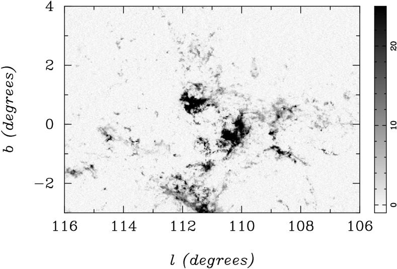
Figure 1: An image of velocity integrated CO J=1-0 emission from a section of the Perseus spiral arm of the Milky Way (Heyer etal 1998). The image shows giant molecular clouds, compact globules and flocculent features.

In this summary of the two sessions on Turbulence in the Interstellar Medium, we will describe important requirements in comparing observations with models of turbulence and the need for future observations and theoretical advances to make progress in this critical field.

2 A Common Platform

A pre-requisite for any useful dialogue between observers and theorists is a common description of the ISM. The ISM and the output from computational studies are best described by 3-dimensional scalar (ex. density, temperature) and vector (ex. velocity, magnetism) fields. However, spectroscopic observations do not directly yield such 3D fields but rather, spectra of a given molecular or atomic transition at different positions in the plane of the sky. The spectrum is a complex integration of scalar and vector field quantities along the line of sight and in principle, provides a valuable diagnostic to these fields. In practice, it is very difficult to reliably extract this information. For a turbulent medium, there is a complex re-ordering of the information into the spectrum that precludes an accurate re-construction of the original fields. In addition, spectroscopic observations are subject to selection effects such as line excitation, opacity, and instrumental noise. These biases act to mask an uncertain fraction of the volume from the observer and are not generally considered when parameterizing 3D model fields (ex. power spectra of the velocity field) or developing predictions. Since it is not possible to uniquely recover the intrinsic fields of density or velocity from the observed spectra, it is necessary to compute synthetic spectra from the model fields with the same observational biases to achieve a common platform to compare with real measurements. Many investigators have recognized this requirement and have developed methods to transform model fields into synthetic spectra taking into account radiative transfer and line excitation (Falgarone etal 1994; Padoan etal 1998; Brunt & Heyer 2002, Padoan, Goodman, & Juvela 2003).

Diagnostics of turbulence which are not based on spectroscopy yield valuable complementary information, but are subject to their own uncertainties. Following the original suggestion by Chandrasekhar & Münch (1950) that the statistics of stellar extinction could be used to probe the underlying density distribution of turbulent interstellar gas, Elmegreen (1997) discussed the distribution of column densities in a fractal model, and Padoan & Nordlund (1999) and Ostriker, Stone, & Gammie (2001) did the same for numerical models of supersonic MHD turbulence. As the latter set of authors have discussed, spatially and dynamically distinct structures are frequently projected on top of one another, possibly suggesting an intrinsic limitation on the use of such statistics for extracting volumetric quantities.

3 Calibrated Spatial Statistics

Images of molecular line emission from interstellar clouds exhibit a wide range of structural features and textures (see Figure 1). The measured spatial variability arises from the various processes that modify the gas phase (UV fields from massive stars), compress (shocks from outflows, HII regions, or turbulence), redistribute the gas (turbulent eddys), or modulate chemical abundances. While it is tempting to investigate interesting, targeted features, such phenomenological efforts do not often generate quantitative constraints to theoretical descriptions of the ISM. Within a turbulent medium, where structure can be generated by advection of material through the velocity field, localized, high contrast objects may be short-lived and therefore, do not evolve to higher density configurations that lead to the formation of stars (see Ballesteros-Paredes etal 1999).

Spatial statistics provide a condensed, unbiased description of observational and model data and are an essential tool for the study of interstellar turbulence. A frequently used example is the power spectrum of the velocity field, which is often further parameterized by the slope of the power law fit. It is essential that any proposed metric derived from the observations reflect the true statistics of interstellar quantities. One can not assume that there is a direct equivalence given the complexities of the projection described above. Therefore, it is necessary to calibrate the metric against fields with known statistics prior to its application on real data. This calibration enables the following results.

• Demonstrate sensitivity to varying true field statistics. A derived metric that is invariant under varying conditions is simply not useful to compare with models.

• Empirically define the algebraic relationship between the true and measured values as this can be distorted in the projection process.

• Evaluate the role of noise, resolution, sample size, and selection effects on the results.

Several semi-calibrated methods have been developed to estimate the scale dependence of the velocity dispersion from spectroscopic data cubes as parameterized by the power law slope of the second order structure function, or equivalently, the energy spectrum ($E(k)\sim k^{-\beta}$) (Miesch, Scalo, & Bally 1999, Lazarian & Pogosyan 2000; Brunt & Heyer 2002). However, the accuracy of these methods is not yet sufficient ($\sigma_{\beta}\sim 0.3$) to even fully distinguish between incompressible Kolmogorov turbulence ($\beta=5/3$) and shock dominated Burgers turbulence ($\beta=2$).

In comparison to the use of velocity statistics, diagnostics of turbulence in molecular clouds based on magnetic field measurements are in their infancy. Polarimetric maps of star-forming regions in the far-infrared probe the orientation of the magnetic field in regions of high extinction (Hildebrand et. al. 2000). The dispersion of the orientation angle about the mean contains information about the fieldstrength (Chandrasekhar & Fermi 1953) as well as the fluctuation spectrum, but corrections for line of sight and angular averaging can be substantial (Heitsch et al. 2001, Ostriker, Stone, & Gammie 2001). This is demonstrated in Figure 2.

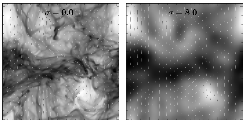
Figure 2: Surface density plots and overlaid polarization vectors for a 256³ simulation of MHD turbulence driven on global scales. The sonic and Alfvén Mach numbers are 10 and 3.2, respectively. The left panel shows unsmoothed data, and the right panel shows the effect of smoothing with a Gaussian filter with $\sigma=8$ pixels. After Heitsch et al. 2001.

Detailed statistical analysis of polarimetric observations of the type emulated in the figure requires more highly resolved spatial sampling than is currently available, but would be quite feasible, for example, with measurements at 100$\mu m$ made by SOFIA.

4 Summary and Future Efforts

The discussions that followed the presentations in this session focused upon the most essential measurements to conduct in order to constrain models and augment our current understanding of interstellar turbulence.

Mass to Magnetic Flux Ratio – The magnetic field is expected to be frozen to the plasma component of interstellar gas, except on the smallest scales. Unless the Alfvén Mach number of the turbulence is much less than unity, which is unlikely to be the case, one expects a statistical correlation between fieldstrength and gas density. Parameterizing the correlation by a power law exponent $\alpha\equiv d\ln{B}/d\ln{\rho}$, one expects $\alpha\sim 2/3$ for very weak fields, and $\alpha\sim 1/2$ for self gravitating clouds supported by moderately strong fields. Published observations of the $B-\rho$ relation suggest that the power law scaling is more an upper envelope than a tight relationship, but the number of data points is small, and corrections due to line of sight averaging and unresolved angular structure could be substantial. But the absence of a $B-\rho$ relation, if confirmed, is evidence for anomalously strong diffusion in the ISM, possibly turbulent in nature (Zweibel 2002, Fatuzzo & Adams 2002, Kim & Diamond 2002, Heitsch et al. in these Proceedings).

The mass to magnetic flux ratio $M/\Phi$ is the global counterpart of the density - fieldstrength relation. It measures the degree to which the evolution of a self gravitating mass element of the ISM is regulated by its magnetic field. If $M/\Phi$ is above the critical value $(M/\Phi)_{c}\sim 0.2G^{-1/2}$, the magnetic field cannot prevent collapse. Measuring the degree of criticality of dense interstellar clouds is necessary in order to determine the dynamical role of magnetic fields in star formation. Observations to date suggest that this ratio, while not far from critical, generally exceeds the critical value (Crutcher 1999 and these Proceedings, Bourke et al. 2001, Crutcher, Heiles, & Troland 2003). Possibly this again is evidence for turbulent diffusion, although these measurements too are subject to small number statistics, line of sight averaging, and resolution effects.

In order to make further progress, it is imperative to obtain direct, reliable observations of the magnetic field strength. In weakly ionized regions this requires measuring Zeeman splitting (difficult), and, in regions with substantial electron density, Faraday rotation. Measurements of the polarization of the far infrared continuum and of radio frequency spectral lines furnish information about the orientation of the field, but not the strength, except indirectly. Reliable measurements of the gas density are required as well; in too many cases one has only column densities, not volume densities. Observing more sources, even if only to obtain upper limits, would improve the statistical reliability of the results. Papers by Crutcher and by Heiles in these Proceedings discuss the situation in molecular and neutral atomic gas, respectively.

It is equally imperative that theoretical models of the $B-\rho$ relation develop observationally testable predictions. For models of turbulent diffusion, this might involve characterizing the turbulent velocity fields, or predicting the structure function for the magnetic fieldstrength or the Stokes parameters. Quantifying the effects of numerical diffusion is a separate but equally important issue in simulations of magnetic field evolution in turbulent media.

Degree of Intermittency - Intermittency describes the filling factor or sparseness of the spatial and temporal dissipation of turbulent energy. Signatures to intermittency include non-gaussian probability density functions (PDFs) of velocity increments (Lis etal 1996; Miesch, Scalo, & Bally 1999; Pety & Falgarone 2003) and the curvature of the scaling exponent, ${\zeta}(q)$, with q where

$$S_{q}(L)=<|{\delta}v|^{q}>\propto L^{{\zeta}(q)}$$

is the generalized structure function and ${\delta}v$ refers to the velocity difference between two points in a volume separated by size scale, $L$. It would be useful to understand the dissipation process as this is a critical step to the formation of stars. At what scales and through which modes is turbulent energy dissipated? Is this energy replenished? If so, what are the primary sources of energy injection to the interstellar cloud (see Miesch & Bally 1994)? The structure function of velocity fluctuations provides a statistical road-map of energy flow within a volume. Principal Component Analysis (Brunt etal 2003) and Velocity Channel Analysis (Lazarian & Pogasyan 2000) can recover the low order moments of the structure function. However, intermittent phenomena are more readily measured within the higher order moments. The complete evaluation of the generalized structure function requires the development of observations and analysis tools that are sensitive to these higher order ($q>2$) velocity fluctuations.

Density Contrast – Collisions of super-Alfvenic gas streams produce shocks and filamentary density distributions. Such filaments are prominent features within the density fields generated by numerical simulations of compressible interstellar turbulence. The measured angular distribution of molecular line emission is not so readily characterized by filaments. Rather, there are filaments, compact cores, flocculent clouds, and diffuse features. Where are the signatures of hydrodynamic shocks? Are these lost in the projection of the fields or in the observational noise? An important metric to develop is a filamentary index which could describe the fraction of mass contained in filaments or sheets both in 3-dimensional density fields and projected images of gas column density.

As stated in the first section of this article, analytical theories of turbulence in the ISM led to a few testable predictions, but do not describe the wealth of detail that observations of the ISM reveal. This made it difficult, in the past, to argue that we understand very basic problems, such as the nature of energy injection, the primary mechanisms for cloud formation, the dynamical role of magnetic fields, and the origin of the observed IMF. Numerical simulations offer a threefold opportunity in this regard. First of all, numerical simulations can be used to study universal problems in data analysis and interpretation, such as recovery of 3D distributions from 2D projections, the role of finite angular resolution, and the role of noise. Studies of this type can be valuable in the interpretation of the observations, and perhaps can lead to new methods of data analysis. Second, it is possible, through parameter studies, to determine the sensitivity of the basic output - the density, velocity, and magnetic fields in a turbulent simulation - to changes in the basic physical input. For example, if turbulence is driven at a particular scale, is that scale imprinted on the output fields? Does it make a difference whether the driving is through addition of energy, or momentum? What is the effect of underlying rotational shear? Finally, the first and second avenues of investigation must be combined to demonstrate the sensitivity, or lack thereof, of observable quantities to physical processes and input parameters. This makes it possible to answer questions such as: What observations are required to determine whether the turbulence in a molecular cloud is driven or decaying? Is there a way to determine, short of direct measurement, whether the magnetic field in a cloud is weak or strong? What is the physical significance of the observed linewidth - size and column density - size relations? We are challenged by these and other questions regarding interstellar turbulence. The continued creative tension between observations and theory provides motivation for future studies to address these critical issues.