Approximate angular diameter distance in a locally inhomogeneous universe with nonzero cosmological constant

We discuss the general and approximate angular diameter distance in the Friedman-Robertson-Walker cosmological models with nonzero cosmological constant. We modify the equation for the angular diameter distance by taking into account the fact that locally the distribution of matter is non homogeneous. We present exact solutions of this equation in a few special cases. We propose an approximate analytic solution of this equation which is simple enough and sufficiently accurate to be useful in practical applications.

1 Introduction

Recent observations of the type Ia supernovae and CMB anisotropy strongly indicate that the total matter-energy density of the universe is now dominated by some kind of vacuum energy also called ”dark energy” or the cosmological constant $\Lambda$ (Perlmutter (1997); Perlmutter et al. (1999); Riess et al. (1998); Riess (2000)). The origin and nature of this vacuum energy remains unknown. There are several review articles providing thorough discussion of the history, interpretations and problems connected with the vacuum energy and observational constrains (Zel’dovich (1967); Weinberg (1989); Carroll et al. (1992)).
The type Ia supernovae have been already observed at redshifts $z>1$. It is well known from galaxy surveys that galaxies and clusters of galaxies up to a scale of $\approx$ 1Gpc are distributed non homogeneously forming filaments, walls and underdense voids. This indicates that on similar scales also the dark matter is distributed non homogeneously. In this paper we analyze the influence of local non homogeneities on the angular diameter distance in a universe with non zero cosmological constant.
The angular diameter distance in a locally non homogeneous universe was discussed by Zeldovich  (Dashveski & Zeldovich (1965)) see also (Dashveski & Slysh (1966)) and (Weinberg (1989); Kayser et al. (1997)). Later Dyer& Roeder (1972) used the so called empty beam approximation to derive an equation for the angular diameter distance; for more detailed references see also (Schneider, Ehlers & Falco (1992)), (Kantowski (1998)), and (Tomita & Futamase (1999)). We follow the Dyer & Roeder method to derive the equation for angular diameter distance in a locally non homogeneous universe with a cosmological constant. In the general case the equation for the angular diameter distance does not have analytical solutions, it can be solved only numerically (Kantowski, Kao & Thomas (2000)). We have found an analytic approximate solution of this equation, which is simple and accurate enough to be useful in practical applications. This allowed us to find an approximate dependence of the angular diameter distance on the basic cosmological parameters.
The paper is organized as follows: we begin with the general form of Sachs equations describing light propagation in an arbitrary spacetime and using the empty beam approximation we derive the equation for angular diameter distance. Then, we discuss the angular diameter distance as observed from a location not at the origin (z=0). Finally, after discussing some properties of the analytical solutions of the equation for the angular diameter distance in a locally non homogeneous universe, we propose an analytic approximation solution of this equation valid in a wide redshift interval (0, 10). We have been motivated by the great advances in observing further and further objects and the construction of very powerful telescopes that provide the possibility to observe gravitational lensing by clusters of galaxies, and supernovae at large distances. It is therefore necessary to develop a more accurate formalism to describe the distance redshift relation and gravitational lensing by high–redshift objects. To achieve this goal we use cosmological models with realistic values of the basic cosmological parameters such as the Hubble constant and the average matter-energy density. In concluding remarks we summarize our results and discuss some perspectives .

2 Propagation of light and local non homogeneities

2.1 General considerations

Let us consider a beam of light emanating from a source S in an arbitrary spacetime described by the metric tensor $g_{\alpha\beta}$. The light rays propagate along a null surface $\Sigma$, which is determined by the eikonal equation

$$g^{\alpha\beta}\Sigma,_{\alpha}\Sigma,_{\beta}=0.$$ (1)

A light ray is identified with a null geodesic on $\Sigma$ with the tangent vector $k_{\alpha}=-\Sigma,_{\alpha}$. The light rays in the beam can be described by $x^{\alpha}=x^{\alpha}(v,y^{a})$, where $v$ is an affine parameter, and $y^{a}$ (a=1, 2, 3) are three parameters specifying different rays. The vector field tangent to the light ray congruence, $k^{\alpha}=\displaystyle{{dx^{\alpha}\over dv}}=-\Sigma,_{\alpha}$, determines two optical scalars, the expansion $\theta$ and the shear $\sigma$, which are defined by

$$\theta\equiv{1\over 2}{k^{\alpha}}_{;\alpha},\;\ \ \ \ \sigma\equiv k_{\alpha;\beta}{\bar{m}}^{\alpha}{\bar{m}}^{\beta},$$ (2)

where ${\bar{m}}^{\alpha}={1\over\sqrt{2}}(\xi^{\alpha}-i\eta^{\alpha})$ is a complex vector spanning the spacelike 2-space (the screen space) orthogonal to $k^{\alpha}$ $(k^{\alpha}{\bar{m}}_{\alpha}=0)$. Since $k_{\alpha}=-\Sigma,_{\alpha}$ the vorticity connected with the light beam is zero in all our considerations; therefore in this case $\sigma$ and $\theta$ fully characterize the congruence. These two optical scalars satisfy the Sachs (Sachs & Kristian (1966)) propagation equations

$$\dot{\theta}+\theta^{2}+|\sigma|^{2}=-\frac{1}{2}R_{\alpha\beta}k^{\alpha}k^{\beta},$$ (3)

$$\dot{\sigma}+2\theta\sigma=-\frac{1}{2}C_{\alpha\beta\gamma\delta}{\bar{m}}^{\alpha}k^{\beta}{\bar{m}}^{\gamma}k^{\delta},$$ (4)

where dot denotes the derivative with respect to $v$, $R_{\alpha\beta}$ is the Ricci tensor, and $C_{\alpha\beta\gamma\delta}$ is the Weyl tensor. Eqs. (3) and (4) follow from the Ricci identity. The optical scalars $\theta$ and $\sigma$ describe the relative rate of change of an infinitesimal area A of the cross section of the beam of light rays and its distortion. The expansion $\theta$ is related to the relative change of an infinitesimal surface area $A$ of the beam’s cross section by

$$\theta={1\over 2}{d\ln{A}\over dv}.$$ (5)

Let us use these equations to study the propagation of light in the Friedman-Robertson-Walker (FRW) spacetime. The FRW spacetime is conformally flat, so that $C_{\alpha\beta\gamma\delta}=0$. From Eq. (4) it follows that, in the FRW spacetime if the shear of the null ray congruence is initially zero, then it always vanishes. Therefore, assuming that the light beam emanating from the source S has vanishing shear, we can disregard the shear parameter altogether (empty beam approximation). Using Eq. (5) we can rewrite equation (3) in the form

$$\ddot{\sqrt{A}}+{1\over 2}R_{\alpha\beta}k^{\alpha}k^{\beta}\sqrt{A}=0.$$ (6)

An observer moving with the 4-velocity vector $u^{\alpha}$ will associate with the light-ray a circular frequency $\omega=cu^{\alpha}k_{\alpha}$. Different observers assign different frequencies to the same light ray. The shift of frequency, as measured by an observer comoving with the source and an arbitrary observer, is related to their relative velocity or the redshift $z$ by

$$1+z={\omega\over\omega_{o}}={c\over\omega_{o}}u_{\alpha}k^{\alpha},$$ (7)

where $\omega$ is the frequency measured by a comoving observer and $\omega_{0}$ by an arbitrary observer. Differentiating this equation with respect to the affine parameter $\it{v}$, we obtain

$${dz\over dv}={c\over\omega_{o}}k^{\alpha}k^{\beta}u_{\alpha;\beta}.$$ (8)

Since the angular diameter distance D is proportional to $\sqrt{A}$ we can rewrite Eq.(6) using D instead of $\sqrt{A}$ and, at the same time, replace the affine parameter $\it{v}$ by the redshift $z$; we obtain

$$\left(\frac{dz}{dv}\right)^{2}\frac{d^{2}D}{dz^{2}}+\left(\frac{d^{2}z}{dv^{2}}\right)\frac{dD}{dz}+\frac{4\pi G}{c^{4}}T_{\alpha\beta}k^{\alpha}k^{\beta}D=0,$$ (9)

where we have used the Einstein equations to replace the Ricci tensor by the energy-momentum tensor. A solution of Eq. (9) is related to the angular diameter distance if it satisfies the following initial conditions:

$$D(z)\arrowvert_{z=0}=0,$$

(10)

$$\frac{dD(z)}{dz}\arrowvert_{z=0}=\frac{c}{H_{0}}.$$

2.2 The angular diameter distance between two objects at different redshifts

In order to use solutions of the Eq. (9) to describe gravitational lenses we have to introduce the angular diameter distance between the source and the lens $D(z_{l},z_{s})$, where $z_{l}$ and $z_{s}$ denote correspondingly the redshifts of the lens and the source. Let $D(z_{1},z_{2})$ denote the angular diameter distance between a fictitious observer at $z_{1}$ and a source at $z_{2}$; of course, $D(0,z)=D(z)$. Suppose that we know the general solution of Eq. (9) for $D(z)$, which satisfies the initial conditions (2.1); let us define $D(z_{1},z)$ by

$$D(z_{1},z)=\frac{c}{H_{0}}(1+z_{1})D(z_{1})D(z)\left|\int_{z_{1}}^{z}{\frac{dz^{\prime}}{D^{2}(z^{\prime})g(z^{\prime})}}\right|\ ,$$ (11)

subject to the conditions

$$D(z_{1},z)\arrowvert_{z=z_{1}}=0,$$

(12)

$$\frac{d}{dz}D(z_{1},z)\arrowvert_{z=z_{1}}={\rm sign}(z-z_{1})\frac{c}{H_{0}}\frac{1+z_{1}}{g(z_{1})}.$$

We see that $D(z_{1},z)$ satisfies Eq. (9), if the function $g(z)$ is a solution of the equation

$$\frac{d}{dz}\ln{g(z)}={\frac{{\large d^{2}z}}{{\large dv^{2}}}\over\left(\frac{{\large dz}}{{\large dv}}\right)^{2}},$$ (13)

so that

$$g(z)=g_{0}\exp{\int{\frac{\frac{d^{2}z^{\prime}}{dv^{2}}}{\left(\frac{dz^{\prime}}{dv}\right)^{2}}dz^{\prime}}},$$ (14)

where $g_{0}$ is an arbitrary constant of integration. It is easy to relate the function $g(z)$ to the Hubble function $H(z)$. In fact, using

$$\frac{dz}{dt}=-(1+z)H(z),$$ (15)

and

$${dz\over dv}=(1+z)^{2}\frac{H(z)}{H_{0}},$$ (16)

it follows that Eq. (13) can be rewritten as

$$\frac{d}{dz}\ln{g(z)}=\frac{d}{dz}\left[\ln{(1+z)^{2}\frac{H(z)}{H_{0}}}\right],$$ (17)

so,

$$g(z)=(1+z)^{2}\frac{H(z)}{H_{0}},$$ (18)

where we have imposed the initial condition $g(0)=1$. Let us remind that one of the Friedman cosmological equations can be rewritten as

$$H(z)=H_{0}\sqrt{\Omega_{m}(1+z)^{3}+\Omega_{k}(1+z)^{2}+\Omega_{\Lambda}},$$ (19)

where $H_{0}$ is the present value of the Hubble constant, $\Omega_{m}=\displaystyle{{8\pi G\varrho_{m}}\over 3H_{0}}$ is the matter density parameter, $\Omega_{k}=-\displaystyle{kc^{2}\over{R_{0}^{2}H_{0}}}$ is the curvature parameter and $\Omega_{\Lambda}=\displaystyle{{\Lambda c^{2}}\over 3H_{0}}$ is the cosmological constant parameter. The omega parameters satisfy a simple algebraic relation

$$\Omega_{m}+\Omega_{k}+\Omega_{\Lambda}=1.$$ (20)

The initial conditions (2.2) expressed in terms of $H(z)$ become

$$D(z_{1},z)\arrowvert_{z=z_{1}}=0,$$ (21)

$$\frac{d}{dz}D(z_{1},z)\arrowvert_{z=z_{1}}={\rm sign}(z-z_{1})\frac{c}{(1+z_{1})H(z_{1})}.$$ (22)

2.3 The angular diameter distance

To apply the angular diameter distance to the realistic universe it is necessary to take into account local inhomogeneities in the distribution of matter. Unfortunately, so far an acceptable averaging procedure for smoothing out local inhomogeneities has not been developed (Krasinski (1997)). Following Dyer & Roeder  (Dyer & Roeder (1972)), we introduce a phenomenological parameter $\alpha=1-{\varrho_{clumps}\over<\varrho>}$ called the clumpiness parameter, which is related to the amount of matter in clumps relative to the amount of matter distributed uniformly (Dashveski & Zeldovich (1965); Tomita et al. (1999)). Therefore, Eq. (9), in the FRW case, can be rewritten in the form

$$\left(\frac{dz}{dv}\right)^{2}\frac{d^{2}D}{dz^{2}}+\left(\frac{d^{2}z}{dv^{2}}\right)\frac{dD}{dz}+\frac{3}{2}\alpha\Omega_{m}(1+z)^{5}D=0.$$ (23)

Let us note however that this equation does not fully describe the influence of non homogeneities in the distribution of matter on the propagation of light. It takes into account only the fact that in locally non homogeneous universe a light beam encounters less matter than in the FRW model with the same average matter density. Equation (23) does not include the effects of shear, which in general is non zero in a locally non homogeneous universe (see, for example SEF Chapter 4 and 11). The effects of shear have been estimated with the help of numerical simulations (see, for example Schneider & Weiss (1988), Linder (1998), Jaroszynski (1991), Watanabe & Sasaki (1990)) but satisfactory analytic treatment is still lacking.

It is customary to measure cosmological distances in units of $c/H_{0}$, therefore we introduce the dimensionless angular diameter distance $r=DH_{0}/c$. Using Eq. (16) and Eq. (19), we finally obtain

$$(1+z)\left[\Omega_{m}(1+z)^{3}+\Omega_{k}(1+z)^{2}+\Omega_{\Lambda}\right]{d^{2}r\over dz^{2}}+$$ (24)

$$\left({7\over 2}\Omega_{m}(1+z)^{3}+3\Omega_{k}(1+z)^{2}+2\Omega_{\Lambda}\right){dr\over dz}$$

$$+{3\over 2}{\alpha}\Omega_{m}(1+z)^{2}r=0,$$

with initial conditions

$$r(z)\arrowvert_{z=0}=0,$$ (25)

$$\frac{dr(z)}{dz}\arrowvert_{z=0}=1.$$ (26)

Eq. (24) can be cast into a different form by using $u=1/{(1+z)}$ as an independent variable instead of $z$; we get

$$u^{2}(\Omega_{m}+\Omega_{k}u+\Omega_{\Lambda}u^{3}){d^{2}r\over du^{2}}-u({3\over 2}\Omega_{m}+\Omega_{k}u){dr\over du}$$

$$+{3\over 2}{\alpha}\Omega_{m}r=0.$$ (27)

On the other hand, using the cosmic time $t$ as an independent variable, Eq. (23) assumes the form

$${d^{2}r\over dt^{2}}-H(t){dr\over dt}+4\pi G{\alpha}\varrho_{m}(t)r=0.$$ (28)

This equation was for the first time introduced by Dashevski & Zeldovich (Dashveski & Zeldovich (1965)) (see also Dashveski & Slysh (1966)), and more recently Kayser et al. (Kayser et al. (1997)) and  (Kantowski (1998)) have used it to derive an equation similar to Eq. (2.3). In Eq. (28) the clumpiness parameter $\alpha$ is usually considered as a constant. However, in (Dashveski & Zeldovich (1965) and Kayser et al. (1997)), $\alpha$ is allowed to vary with time, but only the case $\alpha=$ constant is really considered. For a discussion of the general case when $\alpha$ depends on $z$ see, for example, the paper by Linder (Linder (1988)).
To give an example of our procedure of constructing the angular diameter distance between a fictitious observer at $z_{1}$ and a source at $z_{2}$, let us consider the simple case of $\alpha=$ constant,  $\Omega_{\Lambda}=0$, and $\Omega_{k}=0$. In this case it is easy to integrate the equation (22), we obtain

$$r(z)={{(1+z)^{\beta}-(1+z)^{-\beta}}\over{2\beta(1+z)^{5/4}}},$$ (29)

where $\beta={1\over 4}\sqrt{25-24\alpha}$, is the general solution of Eq. (2.3) with the imposed initial conditions. This solution can be found, for example, in SEF (Schneider, Ehlers & Falco (1992)), (see Eq. (4.56) there). The function $g(z)$ can be easily computed in the flat $\Lambda=0$ Friedman-Robertson-Walker cosmological model; in fact, in this case we have

$$H(z)=H_{0}(1+z)\sqrt{z+1},$$ (30)

so that, according to the Eq. (18), we have

$$g(z)=(1+z)^{3}\sqrt{z+1}.$$ (31)

Thus using (11), we get the familiar solution

$$D(z_{l},z_{s})=\frac{1}{2\beta}\left[\frac{(1+z_{2})^{\beta-\frac{5}{4}}}{(1+z_{1})^{\beta+\frac{1}{4}}}-\frac{(1+z_{1})^{\beta-\frac{1}{4}}}{(1+z_{1})^{\beta+\frac{5}{4}}}\right],$$ (32)

found in SEF.

3 Exact solutions

In the general form the Eq. (24) is very complicated. From the mathematical point of view this equation is of Fuchsian type with four regular singular points and a regular singular point at infinity (Ince (1964)). General properties of this equation have been extensively studied by Kantowski (Kantowski (1998); Kantowski, Kao & Thomas (2000); Kantowski & Thomas (2001)).
Following Kantowski let us cast the Eq. (24) into a different form replacing $1+z=x$ and introducing $r(z)={h(z)\over{1+z}}$, we obtain

$$\left(\Omega_{m}x^{3}+\Omega_{k}x^{2}+\Omega_{\Lambda}\right){d^{2}h\over dx^{2}}+\left({3\over 2}\Omega_{m}x+\Omega_{k}\right)x{dh\over dx}+$$ (33)

$$\left({3\over 2}(\alpha-1)\Omega_{m}x-\Omega_{k}\right)h=0.$$

When $\Omega_{k}\not=0$ by rescaling $x$,  $x={\Omega_{k}\over\Omega_{m}}{\tilde{x}}$ this equation can be turned into the Heun equation

$$({\tilde{x}}^{3}+{\tilde{x}}^{2}+{{\Omega_{\Lambda}\Omega_{m}^{2}}\over\Omega_{k}^{3}}){d^{2}h\over d{\tilde{x}}^{2}}+({3\over 2}{\tilde{x}}+1){\tilde{x}}{dh\over d{\tilde{x}}}+$$

$$[{3\over 2}(\alpha-1){\tilde{x}}-1]h=0.$$ (34)

The angular diameter distance can be expressed in terms of basic solutions of the Heun equation as

$$r(z)={h({\Omega_{m}\over\Omega_{k}}(1+z))\over{1+z}},$$ (35)

provided that $h({\Omega_{m}\over\Omega_{k}})=0$ and $h^{\prime}({\Omega_{m}\over\Omega_{k}})={\Omega_{k}\over\Omega_{m}}$. The generic solution for the angular diameter distance expressed in terms of the Heun functions is very complicated, in an explicit form it is given by Kantowski (Kantowski (1998)).
When $\Omega_{k}=0$, dividing Eq. (33) by $\Omega_{m}$, we obtain

$$(x^{3}+{\Omega_{\Lambda}\over\Omega_{m}}){d^{2}h\over dx^{2}}+{3\over 2}x^{2}{dh\over dx}+{3\over 2}(\alpha-1)xh=0.$$ (36)

By changing variables to $\eta(x)=\sqrt{1+\displaystyle{\Omega_{\Lambda}\over{\Omega_{m}x^{3}}}}$ and introducing new independent variable $P(x)=x^{3/4}h(x)$ this equation can be transformed into the associated Legendre equation

$$(1-\eta^{2}){d^{2}P\over d\eta^{2}}-2\eta{dP\over d\eta}-{1\over 36}(5+{{25-24\alpha}\over{(1-\eta^{2})}})P=0.$$ (37)

In this case ($\Omega_{k}=0$) the angular diameter distance is given by

$$r(z)={2\Gamma(1-{\delta\over 6})\Gamma(1+{\delta\over 6})\over{\delta}}(1+z)^{-{1/4}}\sqrt{1+{\Omega_{\Lambda}\over\Omega_{m}}}{\times}$$ (38)

$$\left[P^{\delta\over 6}_{-{1\over 6}}\left(\sqrt{1+{\Omega_{\Lambda}\over\Omega_{m}(1+z)^{3}}}\right)P^{-{\delta\over 6}}_{-{1\over 6}}\left(\sqrt{1+{\Omega_{\Lambda}\over\Omega_{m}}}\right)-\right.$$

$$\left.P^{\delta\over 6}_{-{1\over 6}}\left(\sqrt{1+{\Omega_{\Lambda}\over\Omega_{m}}}\right)P^{-{\delta\over 6}}_{-{1\over 6}}\left(\sqrt{1+{\Omega_{\Lambda}\over{\Omega_{m}(1+z)^{3}}}}\right)\right],$$

where $\delta=\sqrt{25-24\alpha}$, and $P^{\mu}_{\nu}(z)$ denotes the associated Legendre function of the first kind. In section 5 we will propose a simple approximate analytic solution of the general equation for the angular diameter distance which is reproducing reasonably well the exact numerical solution in the range of redshifts (0, 10) far exceeding the range of redshifts of observed supernovae of type Ia.

4 Angular diameter distances in the gravitational lensing theory.

The angular diameter distances, or their combinations, appear in the main equations and in the most important observational quantities of the gravitational lensing (GL) theory. This fact, together with the relation between the angular diameter distance $(D_{A})$ and the luminosity distance $(D_{L})$

$$D_{L}=\left(1+z\right)^{2}D_{A},$$ (39)

makes the study of the equation for the angular diameter distance still more important, also from the point of view of better interpretation of observational data. In this section we describe very briefly the role of angular diameter distance in the gravitational lensing theory, mentioning only some effects in which it plays an important role.
Let us begin with the general expression for the time delay between different light rays reaching the observer

$$c\Delta t=(1+z_{d})\left\{\frac{D_{d}D_{s}}{D_{ds}}(\@vec{\theta}-\@vec{\beta})^{2}-\psi(\@vec{\xi})\right\}+{\rm constant},$$ (40)

where $D_{d}$, $D_{s}$ and $D_{ds}$ are correspondingly the angular diameter distances to the deflector, to the source and between the deflector and the source. The term $(\@vec{\theta}-\@vec{\beta})$ in Eq. (40) represents the geometrical time delay and the other term is connected with the non homogeneous distribution of matter (Schneider, Ehlers & Falco (1992)). The first term in Eq. (40) is proportional to an important combination of angular diameter distances namely, to $\displaystyle\frac{D_{d}D_{s}}{D_{ds}}$. This combination of angular diameter distances was introduced for the first time by Refsdal (Refsdal (1966)), and was used to obtain an estimate of $H_{0}$ from the time delay measurements of multiply imaged quasars. It is possible to rewrite it in the following way

$$(1+z_{d})\frac{D_{d}D_{s}}{D_{ds}}=\frac{c}{H_{0}}[\chi(z_{d})-\chi(z_{s})]^{-1}\ ,$$ (41)

where the function $\chi$ is given by

$$\chi(z,\Omega_{m},\Omega_{\Lambda},\Omega_{k},\alpha) \equiv \int_{z}^{\infty}{\frac{dz}{r^{2}g(z)}}=$$ (42)

$$\int_{z}^{\infty}{{H_{0}\over{r^{2}(z)(1+z)^{2}H(z)}dz}}.$$

So, $\chi$ is connected with the general solution of Eq. (2.3), and it directly appears in the expression for time delay.
Let us now consider the cosmological lens equation. The metric describing FRW cosmological models is conformally flat. In this case the simplest way to derive the lens equation is to use the Fermat principle, so we have

$$\frac{\partial\Delta t}{\partial\@vec{\theta}}=0,$$ (43)

or

$$\@vec{\beta}=\@vec{\theta}-\frac{2R_{g}}{cH_{0}}(1+z_{d})[\chi(z_{d})-\chi(z_{s})]\frac{\partial{\psi}}{\partial{\@vec{\theta}}}\ ,$$ (44)

where $R_{g}$ is the Schwarzschild radius of the deflector. By denoting $\@vec{\xi}=D_{d}\@vec{\theta}$, $\@vec{\eta}=D_{s}\@vec{\beta}$, and $\@vec{\alpha}(\@vec{\xi})=\displaystyle{\frac{2R_{g}}{D_{d}}\frac{\partial{\psi}}{\partial{\@vec{\theta}}}}$, we can transform Eq.(44) into

$$\@vec{\eta}=\frac{D_{s}}{D_{d}}\@vec{\xi}-D_{ds}\@vec{\alpha}(\@vec{\xi})\ ,$$ (45)

which is formally identical with the lens equation for $z<<1$. As is apparent, in the lens equation (45) another dimensionless combination of angular diameter distances, $D_{s}/D_{d}$ appears, besides the angular diameter distance itself, $D_{ds}$. In other words, in the equations describing gravitational lensing we find quantities, which can be written in terms of the angular diameter distance $D(z)$ and the $\chi(z)$ function. In the general case $D(z)$ and $\chi(z)$ can be evaluated only numerically. In the next section we propose a simple analytical approximation for both functions. We hope that these approximate forms can be useful, for example, in big numerical codes used to derive basic cosmological parameters from observational data and to study for instance, statistical lensing, weak lensing, microlensing of QSO, etc.

5 The approximate expression for the angular diameter distance

In the generic case the equation (24) does not have analytical solutions (Kantowski (1998); Kantowski, Kao & Thomas (2000)). From the mathematical point of view this equation is of the Fuchsian type (Ince (1964)) with four regular singular points and a regular singular point at infinity. The solutions near each of the singular points, including the point at infinity, are given by the Riemann ${\mathcal{P}}$-symbol and in general the solutions can be expanded in a series of hypergeometric functions (Tricomi (1961)) or expressed in terms of the Heun functions (Kantowski (1998)).
In practice, in the general case, the equation (24) with appropriate initial conditions is solved numerically. In Fig.1 we show a numerical solution of the D-R equation for $\alpha=0.8$, $\Omega_{\Lambda}=0.7$, $\Omega_{k}=0$ and $\Omega_{m}=0.3$.

Figure 1: The dimensionless angular diameter distance as a function of the redshift in a flat cosmological model with $\Omega_{m}=0.3$,  $\Omega_{\Lambda}=0.7$ and $\alpha=0.8$.

Using Mathematica we discovered that there is a simple function $r(z)$ which quite accurately reproduces the exact numerical solutions of the equation (24) for $z$ up to 10, it has the form

$$r(z)=\frac{z}{{\sqrt{d_{1}\,z^{2}+{\left(1+d_{2}\,z+d_{3}\,z^{2}\right)}^{2}}}},$$ (46)

where $d_{1}$, $d_{2}$ and $d_{3}$ are constants which depend on the parameters that specify the considered cosmological model. First of all please note that the function (46) automatically satisfies the imposed initial conditions, so $r(0)=0$ and $\displaystyle{dr\over dz}(0)=1$. To express the constants $d_{1}$, $d_{2}$ and $d_{3}$ in terms of $\Omega_{\Lambda}$, $\Omega_{m}$, $\Omega_{k}$ and $\alpha$ we inserted the proposed form of $r(z)$ into the equation (24) and required that it be satisfied to the highest order. In this way we obtained that:

$$d_{1} = \frac{-\left(2\,\Omega_{k}+3\,\Omega_{m}\right)^{2}}{4}+\frac{7\,\Omega_{k}+\left(13+\alpha\right)\,\Omega_{m}}{2}-$$

$$\frac{14\,\Omega_{k}+\left(28+5\,\alpha\right)\,\Omega_{m}}{6\,\Omega_{k}+7\,\Omega_{m}+4\,\Omega_{\Lambda}},$$

$$d_{2} = 1+\frac{2\,\Omega_{k}+3\,\Omega_{m}}{4},$$ (48)

$$d_{3} = \frac{1}{16}\left(\left(2\,\Omega_{k}+3\Omega_{m}\right)^{2}-4\,\left(5\,\Omega_{k}+9\,\Omega_{m}\right)\right.+$$

$$\left.\frac{8\,\left(14\,\Omega_{k}+\left(28+5\alpha\right)\,\Omega_{m}\right)}{6\,\Omega_{k}+7\,\Omega_{m}+4\,\Omega_{\Lambda}}\right).$$

In Fig. 2 we show the approximate solution of the equation (24) for $\alpha=0.8$, $\Omega_{\Lambda}=0.7$, $\Omega_{k}=0$, and $\Omega_{m}=0.3$ and for comparison we also plot the exact solution.

Figure 2: The exact dimensionless angular diameter distance $r$ is plotted (solid line) and compared with the analytic approximation (dashed line) in a model with $\alpha=0.8$, $\Omega_{\Lambda}=0.7$, $\Omega_{k}=0$ and $\Omega_{m}=0.3$. In the considered range of redshifts the relative error is less than $10\%$.

Using Mathematica we have also found a useful approximate analytical form for the $\chi$ function

$$\chi(z)={1\over{z\left(1+\displaystyle{z\over\gamma}\right)}},$$ (50)

where $\gamma$ is a constant. Unfortunately we have not been able to analytically relate $\gamma$ to $\alpha$ and other cosmological parameters and the appropriate value of $\gamma$ should be obtained by the standard fitting procedure. In Fig. 3 we show the exact numerical solution for $\chi(z)$ and for comparison we plot the approximate solution with the best fit value of $\gamma=6$.

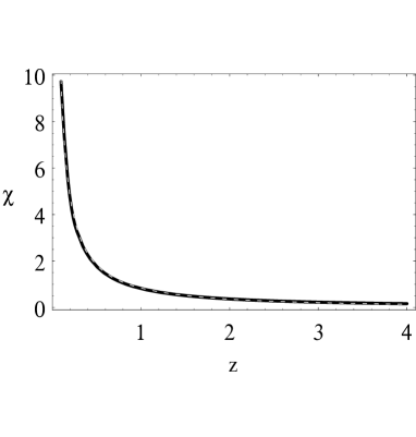
Figure 3: The exact dimensionless function $\chi$ (solid line) for a model with $\alpha=0.8$, $\Omega_{\Lambda}=0.7$, $\Omega_{k}=0$, and $\Omega_{m}=0.3$. With dashed line we plot the analytic approximation with the best fit value of the parameter $\gamma=6$.

6 Conclusions

In this paper we discuss the angular diameter distance in the Friedman-Robertson-Walker cosmological models and consider the case when the cosmological constant and the curvature of space could be different from zero. The effects of local non homogeneous distribution of matter are described by a phenomenological parameter $\alpha$, consistently with the so called empty–beam approximation. Unfortunately, at the moment there are no generally accepted models that describe the distribution of baryonic and dark matter and therefore the influence of inhomogeneities of matter distribution can be included only at this approximate level. In the generic case the equation (24) is of a Fuchsian type, with four regular singular points and one regular singular point at infinity. The general solution of this type of ordinary differential equation is given in terms of the Heun functions (Kantowski (1998); Demianski et al. (2000)).

However the exact solution is so complicated that it is useless in practical applications  (Kantowski (1998); Kantowski, Kao & Thomas (2000)). Therefore we have proposed an approximate analytic solution, simple enough to be used in many applications and at the same time it is sufficiently accurate, at least in the interesting range of redshifts ($0\leq z\leq 10$). In Fig. 2 we compare the exact numerical solution of the equation for the angular diameter distance with the approximate one. The approximate solution reproduces the exact curve quite well and the relative error does not exceed $10\%$.
Following SEF, we have found the function $\chi$ which appears in the expression for time delay as well as in the lens equation, and which naturally appears in the expression for angular diameter distance between two arbitrary objects at redshifts $z_{1}$ and $z_{2}$ ( see Eq. (11)).
We have also proposed an approximate analytical form of the function $\chi$ which depends only on one parameter $\gamma$ but unfortunately $\gamma$ has to be fixed by a standard fitting procedure (see Fig. 3). Our approximations have been already applied in complicated codes used to study the statistical lensing (Perrotta et al. (2001)).
Finally we would like to stress that from our analysis it follows that variations in the angular diameter distance caused by the presence of cosmological constant are quite similar to the effects of a non homogeneous distribution of matter described here by the clumpiness parameter $\alpha$. In Fig. 4 we plot the angular diameter distance for two models, one with a homogeneous distribution of matter ($\alpha=1$) and $\Lambda\not=0$ and another with a non homogeneous distribution of matter ($\alpha=0.7$) and $\Lambda=0$. We see that an inhomogeneous distribution of matter can mimic the effect of a non zero cosmological constant. This is an important observation in view of the recent conclusions based on observations of high redshift type Ia supernovae that the cosmological constant is different form zero  (Perlmutter (1997); Riess (2000)).

Figure 4: The angular diameter distance for two models, one with a homogeneous distribution of matter ($\alpha=1$) and $\Lambda\not=0$ (solid line) and another with a non homogeneous distribution of matter ($\alpha=0.7$) and $\Lambda=0$  (dashed line).

7 Acknowledgments

It is a pleasure to thank V.F. Cardone, G. Covone, C. Rubano, P. Scudellaro, and M. Sereno for the discussions we had on the manuscript. E.P. is partially supported by the P.R.I.N. 2000 SINTESI. This work was supported in part by EC network HPRN-CT-2000-00124. M.D. wants to acknowledge partial support of the Polish State Committee for Scientific Research through grant Nr. 2-P03D-017-14 and to thank the Theoretical Astrophysics Center in Copenhagen for warm hospitality.

8 Appendix

As was already noted the equation for the angular diameter distance in a locally non homogeneous Friedman-Robertson-Walker universe with non zero cosmological constant can be reduced to the Heun equation (see Eq. 28) (Heun, 1889). The Heun differential equation generalizes the Gauss hypergeometric equation, it has one more finite regular singular point (see Ince, 1964). This equation often appears in physical problems in particular in studying of diffusion, wave propagation, heat and mass transfer, and magnetohydrodynamics (see Ronveaux, 1995). In the general form the Heun equation can be written as

$${d^{2}H\over dy^{2}}+\left({a_{1}\over{y-y_{1}}}+{a_{2}\over{y-y_{2}}}+{a_{3}\over{y-y_{3}}}\right){dH\over dy}+$$

$${(a_{4}y-q)\over{(y-y_{1})(y-y_{2})(y-y_{3})}}H=0,$$ (51)

where $a_{1}$, $a_{2}$, $a_{3}$, $a_{4}$, $q$, $y_{1}$, $y_{2}$ and $y_{3}$ are constants, or in a canonical form as (Bateman & Erdélyi (1955))

$$x(x-1)(x-a){d^{2}H\over dx^{2}}+$$

$$\left\{(\alpha+\beta+1)x^{2}-\left[\alpha+\beta+1+a(\gamma+\delta)-\delta\right]x+a\gamma\right\}{dH\over dx}+$$

$$(\alpha\beta x-q)H=0,$$ (52)

where $\alpha$, $\beta$, $\gamma$, $\delta$, $a$, and $q$ are constants.

When $\gamma$ is not an integer, the general solution of the Heun equation can be written as:

$$H(x) = C_{1}F(a,q,\alpha,\beta,\gamma,\delta,x)+$$

$$C_{2}|x|^{1-\gamma}F(a,q_{1},\alpha-\gamma+1,\beta-\gamma+1,2-\gamma,\delta,x),$$

where $C_{1}$ and $C_{2}$ are constants and $q_{1}=q+(\alpha-\gamma+1)(\beta-\gamma+1)-\alpha\beta+\delta(\gamma-1)$.

Following our success in finding an approximate solution of the equation for angular diameter distance we would like to present an approximate solution of the Heun equation. It has the form:

$$H(x)=B\frac{x}{x_{0}}\,\left(\frac{x}{x_{0}}-1\right)$$ (54)

$${1\over{\sqrt{{\left(1+d_{2}\,\left(\frac{x}{x_{0}}-1\right)+d_{3}\,{\left(\frac{x}{x_{0}}-1\right)}^{2}\right)}^{2}+d_{1}\,{\left(\frac{x}{x_{0}}-1\right)}^{2}}}\,},$$

where the parameter $x_{0}$ represents the point where the initial conditions are specified and $d_{1}$, $d_{2}$, $d_{3}$, $B$ are constants. For the Heun equation we adopt the following initial conditions:

$$H[x_{0}] = 0,$$ (55)

$${dH\over dx}\left|{}_{x_{0}}\right. = {B\over x_{0}}.$$ (56)

Please note that the form (8) automatically satisfies the imposed initial conditions.

To express the constants $d_{1}$, $d_{2}$ and $d_{3}$ in terms of $\alpha$, $\beta$, $\gamma$, $\delta$, $a$, and $q$, it is necessary to insert the proposed form of $H(x)$ into the canonical Heun equation (52) and require that it be satisfied to the highest order. The constants $d_{1}$, $d_{2}$ and $d_{3}$ obtained in this way are quite complicated. It will take about 3 pages to give them here. They are shown in an explicit form at http://people.na.infn.it/ ester

Figure 5: Comparison of the exact (solid line) with the approximate solution (dashed line) of the Heun equation.

Figure 6: Relative error of the approximate solution of the Heun equation as a function of $x$.

In Fig. 5 we compare an exact numerical solution of the Heun equation with the approximate solution for the same values of $\alpha$, $\beta$, $\gamma$, $\delta$, $a$ and $q$.

References

- Bateman & Erdélyi (1955) Bateman, H., and Erdélyi, A., Higher Transcedental Functions, Vol. 3, 1955, McGraw-Hill Book Comp., New York
- Carroll et al. (1992) Carroll, S.M., Press, W.H., Turner, E.L., 1992, Ann. Rev. Astro. Astrophys. 30, 499
- Dashveski & Zeldovich (1965) Dashveski V.M., Zeldovich Ya.B., 1965, Soviet Astr., 8, 854
- Dashveski & Slysh (1966) Dashveski V.M., Slysh V.I.,1966, Soviet Astr., 9, 671
- Dyer & Roeder (1972) Dyer C.C., Roeder R.C., 1972, ApJ, 174, L115
- Demianski et al. (2000) Demianski M., de Ritis R. ,Marino A.A., Piedipalumbo E., astro-ph/0004376
- Dyer & Oattes (1988) Dyer C.C.,Oattes L.M., 1988, ApJ, 326,50
- Dashevski & Zeldovich (1965) Dashevski V.M., Zeldovich Y.B., 1965,Soviet. Astr., 8, 854.
- Etherington (1933) Etherington J.M.H., 1933, Phil.Mag., 15, 761
- Heun (1889) Heun, K., 1889, Math.Ann., 33, 161
- Ince (1964) Ince E.L, Ordinary differential equation, 1964, Dover, New York
- Kayser et al. (1997) Kayser R., Helbig P., Schramm T., 1997, A&A, 318, 680
- Kayser & Refsdal (1988) Kayser R., Refsdal S., 1988, A&A, 197, 63K
- Kantowski (1998) Kantowski R., 1998, ApJ, 507,483
- Kantowski, Kao & Thomas (2000) Kantowski R., Kao J.K., Thomas, R.C., 2000, ApJ, 545, 549
- Kantowski & Thomas (2001) Kantowski R., and Thomas, R.C., 2001, ApJ, 561, 491
- Krasinski (1997) Krasinski A., Inhomogeneous Cosmological Models, 1997, Cambridge University Press, Cambridge
- Jaroszynski (1991) Jaroszynski M., 1991, MNRAS, 249, 430
- Linder (1988) Linder E.V.,1988, A&A, 206, 190
- Linder (1998) Linder E.V.,1998, ApJ, 497, 28
- Nakamura (1997) Nakamura T., 1997, Phys. Rev. D, 40, 2502
- Perlmutter (1997) Perlmutter S. et al., 1997, ApJ, 483, 565
- Perlmutter et al. (1999) Perlmutter S. et al., 1999, ApJ, 517, 565
- Perrotta et al. (2001) Perrotta F., Baccigalupi C., Bartelmann M., De Zotti G., Granato G. L., 2002, MNRAS, 329, 445; astro-ph/0101430
- Riess et al. (1998) Riess et al., 1998, AJ, 116, 1009
- Riess (2000) Riess, A.G., 2000, PASP, 112, 1284
- Refsdal (1966) Refsdal S., 1966, MNRAS, 132,105R
- Refsdal (1970) Refsdal S., 1970, ApJ, 159, 357R
- Seitz Schneider & Ehlers (1994) Seitz S.,Schneider P., Ehlers J., 1994, Class.Quant.Grav. 11 2345
- Ronveaux (1995) Ronveaux, A., Heun’s Differential Equation, 1995, Oxford University Press, Oxford
- Sachs & Kristian (1966) Sachs R.K., Kristian, J., 1966, ApJ, 143, 379
- Schneider & Weiss (1988) Schneider P., Weiss A., 1988, ApJ,327, 526
- Schneider, Ehlers & Falco (1992) Schneider P., Ehlers J., Falco E.E., 1992, Gravitational lenses, Springer - Verlag, Berlin
- Tomita & Futamase (1999) Tomita K., Futamase T., Gravitational lensing and the high-redshift universe, 1999, Prog. Theor. Phys., 133
- Tomita et al. (1999) Tomita K., Premadi P., Nakamura T., 1999 Prog. Theor. Phys., 133, 85
- Tricomi (1961) Tricomi F.G., Differential equations, 1961, Blackie, London
- Watanabe & Sasaki (1990) Watanabe K., Sasaki M., 1990, Publ. Astron. Soc. Japan, 42, L33
- Weinberg (1976) Weinberg S., 1976, ApJ, 208, L1
- Weinberg (1989) Weinberg S., 1989, Rev. Mod. Phys., 61, 1
- Zel’dovich (1967) Zeldovich, Ya., B., 1967, Pis’ma Zh. Eksp. Teor. Fiz. 6, 883; (JETP Lett. 6,316 (1967)).