On the Iron content in rich nearby Clusters of Galaxies

In this paper we study the iron content of a sample of 22 nearby hot clusters observed with BeppoSAX. We find that the global iron mass of clusters is tightly related to the cluster luminosity and that the relatively loose correlation between the iron mass and the cluster temperature follows from the combination of the iron mass vs. luminosity and luminosity vs. temperature correlations. The iron mass is found to scale linearly with the intracluster gas mass, implying that the global iron abundance in clusters is roughly constant. This result suggests that enrichment mechanisms operate at a similar rate in all clusters. By employing population synthesis and chemical enrichment models, we show that the iron mass associated to the abundance excess which is always found in the centre of cool core clusters can be entirely produced by the brightest cluster galaxy (BCG), which is always found at the centre of cool core clusters. The iron mass associated to the excess, the optical magnitude of the BCG and the temperature of the cluster are found to correlate with one another suggesting a link between the properties of the BCG and the hosting cluster. These observational facts lends strength to current formation theories which envisage a strong connection between the formation of the giant BCG and its hosting cluster.

1 Introduction

The X-ray thermal continuum observed in clusters of galaxies originates from the hot intra-cluster medium (ICM) permeating the cluster potential well. At the high temperatures measured in rich clusters, kT$\lower 2.15277pt\hbox{$\;\buildrel>\over{\sim}\;$}3$ keV, the ICM is highly ionised and its spectrum presents a number of emission lines, among which the most prominent is the Fe K-shell line at $\sim 7$ keV. From the measure of the equivalent width of these spectral lines it is possible to estimate the abundance of a given element. A well known result is that the global iron abundance in clusters is about a third of the solar value and that this value remains constant within redshift $\lower 2.15277pt\hbox{$\;\buildrel<\over{\sim}\;$}1$ (Mushotzky & Loewenstein 1997, Allen & Fabian 1998, Della Ceca et al. 2000, Ettori, Allen & Fabian 2001, Tozzi et al. 2003), indicating that the enrichment process has mostly taken place at early times in the cluster formation.

The ICM iron mass is a key observable to constrain the integral past star formation history in clusters, and its relation with other observables such as the cluster optical light, total cluster mass and stellar mass allows us to study the enrichment processes and the related efficiencies. The iron mass of the ICM correlates with the optical light of massive early-type galaxies in clusters (Arnaud et al. 1992), suggesting that the stellar population of these systems are the main responsible of the ICM enrichment. Further evidences that clusters evolved experiencing very similar star formation histories comes from the observed constancy of the iron-mass-to-light ratio (Ciotti et al. 1991, Renzini et al. 1993, Renzini 1997), and of the iron-mass-to-total-mass ratio (Lin, Mohr & Stanford 2003) among clusters. These evidences, and the similar global abundance among clusters, support the possibility that rich clusters evolved as ”closed boxes” after their formation, with little baryon exchange with the surroundings (Renzini 1997). While the origin of the metals observed in the ICM is clearly related to stellar evolution (supernovae events), the transfer mechanism of these metals from stars in galaxies to the ICM is less clear. Possible ICM enrichment mechanisms that have been proposed for clusters are: ram pressure stripping of metal enriched gas from cluster galaxies (e.g. Gunn & Gott 1972, Toniazzo & Schindler 2001), and stellar winds AGN- or SN- induced in early-type galaxies during the formation of the proto-cluster (e.g. Gnedin 1998, Kauffmann & Charlot 1998, Dupke & White 2000, Renzini et al. 1993, Lin et al. 2003). The efficiency of the metal extraction by ram pressure stripping should increase with the local density of galaxies, the lack of any trend of either the iron abundance and iron-mass-to-light ratio with cluster temperature or velocity dispersion argues against this being the main mechanisms of metal transportation at work in clusters (Renzini 2003).

Spatially resolved analysis of metal abundances in clusters have become possible only recently, first with ASCA and BeppoSAX and, more recently, with Chandra and XMM-Newton. These measurements have shown that abundance gradients are common in clusters and groups of galaxies (ASCA: Fukazawa et al. 2000, Makishima et al. 2001, Finoguenov, Arnaud & David 2001; BeppoSAX: Irwin & Bregman 2001, De Grandi & Molendi 2001; Chandra: Ettori et al. 2002, Hicks et al. 2002, Schmidt, Fabian & Sanders 2002, Blanton et al. 2003; XMM-Newton: Molendi & Gastaldello 2001, Gastaldello & Molendi 2002, Finoguenov et al. 2002, Pratt & Arnaud 2002, Matsushita, Finoguenov & Boehringer 2003). Relaxed clusters with evidences of cool cores have global abundance about twice larger than the abundance of non relaxed systems (Allen & Fabian 1998). De Grandi & Molendi (2001, DM01 hereafter), found that this is due to the almost ubiquitous presence of abundance peaks in the cores of relaxed clusters in correspondence of the brightest cluster galaxy (BCG), while clusters showing evidences of dynamical activity on large scales have flat abundance profiles. Comparison between the total cluster light and abundance profiles suggests that the abundance peaks are probably due to the accumulation of metal ejection from the BCG in the ICM (Fukazawa et al. 2000, DM01).

The plan of the paper is as follows: in Sect. 2 we describe the sample, give a brief review on the data analysis and discuss the deprojected abundance profiles. In Sect. 3 we compute the ICM iron mass for our clusters and study how this mass scales with the other important physical observables. We estimate the metal content of local clusters and compare it to the cosmological metal budget. In Sect. 4 we investigate the origin of the iron mass excess associated to the abundance peak observed in cool core clusters and its possible connection with the brightest cluster galaxy located at the centre of these clusters. Finally we summarise our findings in Sect. 5.

In the rest of the paper we employ the solar abundance ratios from Grevesse & Sauval (1998) with $Z_{\odot}={\rm Fe/H}=3.16\times 10^{-5}$ by number, as suggested by Brighenti & Mathews (1999). This ”standard solar composition” derived by Grevesse & Sauval (1998) follows from recent photospheric models of the Sun and shows perfect agreement with the meteoritic composition. We recall here that the new abundances can be easily converted into abundances relative to other sets of solar abundances with a simple scaling. The multiplicative factor necessary to convert abundances relative to solar values from Grevesse & Sauval (1998) to those relative to solar values from Anders & Grevesse (1989) is 0.675.

The cosmological framework is an Einstein-de Sitter model with H₀ = 50 Mpc km s^-1 to allow comparison with previous works. Quoted confidence intervals are $68\%$ for 1 interesting parameter (i.e. $\Delta\chi^{2}=1$), unless otherwise stated.

2 The Sample and deprojected Abundance Profiles

We consider a sample of 22 nearby ($z\lower 2.15277pt\hbox{$\;\buildrel<\over{\sim}\;$}0.1$) clusters of galaxies observed with the two Medium Energy Concentrator Spectrometers (MECS) on board BeppoSAX. These clusters cover the range in gas temperature between 3 and 10 keV, and have bolometric X-ray luminosity between $2\times 10^{44}$ erg s^-1 and $6\times 10^{45}$ erg s^-1. We have divided the sample into a subsample of 10 clusters without evidences of cool cores (NCC clusters hereafter, these objects were called non-CF clusters in our previous papers) and another subsample of 12 clusters with cool cores (CC clusters hereafter, they were called CF clusters in our previous papers). We have defined NCC cluster an object with a mass deposition rate consistent with zero according to the spatial analysis of ROSAT observations presented in Peres et al. (1998). Contrary to NCC systems, which show signatures of recent merging events, CC clusters are mostly relaxed systems (at least on the scale of 100 kpc) with evidence of strong emission peaks (e.g. Mohr, Mathiesen & Evrard 1999) and cool gas in their centres (e.g. Peres et al. 1998, Allen, Schmidt & Fabian 2001).

Details on the data analysis and deprojection technique are given in the previous papers of this series, DM01, De Grandi & Molendi (2002) and Ettori, De Grandi & Molendi (2002) (EDM02 in the rest of this paper). The observation log for the current cluster sample is given in Table 1 of EDM02. The observed metal abundance and temperature profiles have been discussed in details in DM01 and De Grandi & Molendi (2002), respectively. We remark here that the metal abundances determined for these clusters are essentially iron abundances derived from the K-shell iron line at $\sim 6.9$ keV, and that the other elements in the ICM are scaled in solar proportion. In EDM02 we have converted the physical quantities derived from the fitting of the MECS spectra extracted from cluster regions projected on the sky, into their deprojected values under the assumption of spherical geometry of the X-ray emitting plasma. For the first time these BeppoSAX observations allowed us to obtain deprojected physical quantities of clusters from one dataset only.

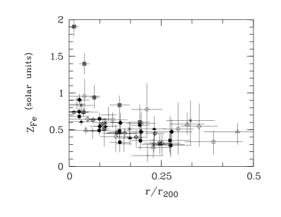
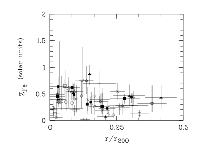
Figure 1: Deprojected iron abundance profiles for CC (left) and NCC (right) clusters plotted as a function of the radius normalised to $r_{200}$. Clusters are related to symbols as follows: (left panel) A85 (filled circles), A426 (asterisks), A496 (filled lozenges), A1795 (filled triangles), A2029 (open squares), A2142 (open triangles), A2199 (filled squares), A3526 (crossed squares), A3562 (open circles), A3571 (crosses $+$), 2A 0335$+$096 (crosses $\times$), and PKS 0745$-$191 (open lozenges); (right panel) A119 (open lozenges), A754 (filled squares), A1367 (open circles), A1656 (open squares), A2256 (filled circles), A2319 (filled triangles), A3266 (open triangles), A3376 (crosses $+$), A3627 (crosses $\times$), and Triangulum Austr. (asterisks).

The projected (observed) metal abundance profiles presented in DM01 provided evidences that CC clusters have strong abundance enhancements in their cores with respect to NCC systems, which on the contrary tend to have constant metallicities. In Fig. 1 we show the deprojected iron abundance profiles for both cluster types, as a function of the radius normalised to $r_{200}$ (values of $r_{200}$ are given in EDM02). The comparison between the deprojected profiles is in agreement with the comparison of projected profiles reported in DM01: NCC systems have almost flat metallicity profiles whereas CC ones have metallicity enhancements in the core and flat profiles in the outermost regions. The best-fit value of the metallicity using a constant model over the whole radial range for both CC and NCC clusters is $0.62\pm 0.01$ and $0.32\pm 0.01$, respectively. The constant model however provides a poor fit in both cases ($\chi^{2}$/dof=302/60 for CC and 112/56 for NCC clusters).

In the case of NCC clusters the fact that the constant model does not reproduce the data adequately is due to the large scatter in their deprojected profiles. We recall that the deprojected profiles are obtained by applying a deprojection technique which assumes that the sources are spherically symmetric, in the case of NCC clusters this is a rather strong simplification and may result in the observed scatter.

In the case of CC clusters the constant model is clearly a poor fit to the profiles. The best-fit to the data with a $\beta$-model, $Z_{\rm Fe}=Z_{\rm Fe0}(1+(x/x_{c}))^{-\alpha}$ where $x=r/r_{200}$, gives $Z_{\rm Fe0}=0.80\pm 0.03$, $x_{\rm c}=0.04\pm 0.01$ and $\alpha=0.18\pm 0.03$ ($\chi^{2}$/dof=140/58), an F-test shows that the improvement with respect to the constant model is highly significant (P${}_{F}>99.99\%$). Note that the metallicity profile of Centaurus cluster (A3526) is peculiar in the sense that the deprojected abundance at its centre is the only one, among our CC clusters, to be larger than solar. By excluding Centaurus both the constant and $\beta$ models fit on the remaining CC clusters give parameters indistinguishable from those obtained considering all CC clusters. The only important difference is that, when Centaurus is excluded, the $\beta$-model becomes acceptable ($\chi^{2}$/dof=69/51).

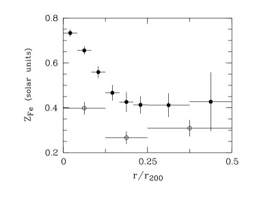
Figure 2: Binned weighted average of the deprojected metallicity profiles for CC (filled circles) and NCC (open circles) clusters.

In Fig. 2 we plot, for both CC and NCC clusters, the binned error-weighted average of the metallicity profiles shown in Fig. 1. From this figure we note that the mean abundance at large radii is different between CC and NCC clusters. The best-fitting constant to the mean profile of CC clusters for $r>0.2\leavevmode\nobreak\ r_{200}$ gives an average abundance of $0.40\pm 0.03$ ($\chi^{2}$/dof=12.4/17), which differs by $\sim 2.2\sigma$ from the average abundance over the whole radial range of NCC clusters ($0.32\pm 0.01$). Although the statistical significance of this difference is small we suggest that this could indicate that CC clusters are older systems than the NCC ones. In this case the early-type galaxy population of CC clusters had more time to produce metals and eject them into the ICM with respect to NCC clusters. An independent indication that relaxed clusters are probably older than disturbed systems, comes from the work of Katayama et al. (2003), who found that the offset of the brightest cluster galaxy from the peak of cluster X-ray emission is larger for younger (i.e. less relaxed) clusters. New XMM-Newton measurements of cluster abundances in the outermost regions of the clusters are required to make further progress on this important issue.

Table 1: Sample of 22 galaxy clusters considered in this study. The ‘CC’ column indicates if a cluster is or is not a cool core object according to the mass deposition rate quoted in Peres et al. (1998). The ICM iron mass computed at different overdensities are reported in the third, fourth and fifth columns. The sixth column reports the iron mass excess measured for CC clusters only.

Cluster	CC	${\rm M_{Fe}}$	${\rm M_{Fe}}$	${\rm M_{Fe}^{(\dagger)}}$	${\rm M_{Fe}^{exc}}$
		${\rm 10^{10}M_{\odot}}$	${\rm 10^{10}M_{\odot}}$	${\rm 10^{10}M_{\odot}}$	${\rm 10^{9}M_{\odot}}$
		$\Delta=2500$	$\Delta=1000$	$\Delta=500$
A85	y	3.90(1.06)	7.83(1.90)	12.1(2.80)	4.10(1.92)
A426	y	2.90(0.31)	4.94(0.47)	7.10(0.63)	3.57(1.43)
A496	y	1.98(0.41)	3.53(0.65)	5.09(0.89)	1.58(0.54)
A1795	y	3.73(0.59)	8.00(1.17)	12.7(1.80)	3.28(1.69)
A2029	y	6.00(1.96)	12.0(3.34)	18.7(4.77)	11.6(5.63)
A2142	y	5.59(1.47)	13.3(3.04)	21.9(4.21)	1.09(0.96)
A2199	y	1.63(0.30)	2.69(0.46)	3.76(0.62)	1.50(0.95)
A3526	y	0.54(0.12)	0.88(0.17)	1.23(0.22)	0.64(0.21)
A3562	y	1.77(0.65)	3.72(1.10)	5.67(1.54)	0.61(0.34)
A3571	y	3.07(0.66)	5.34(1.15)	7.77(1.68)	3.81(1.96)
2A 0335$+$096	y	1.61(0.36)	3.01(0.64)	4.41(0.92)	1.77(0.54)
PKS 0745$-$191	y	5.49(1.23)	12.3(2.69)	20.1(4.22)	4.89(1.43)
A119	n	1.38(0.52)	2.59(0.86)	3.76(1.19)	—
A754	n	3.29(0.93)	9.50(1.70)	16.3(2.55)	—
A1367	n	1.07(0.61)	3.35(1.22)	5.42(1.76)	—
A1656	n	1.23(0.43)	2.27(0.62)	3.31(0.81)	—
A2256	n	2.76(0.74)	7.59(1.30)	12.2(1.84)	—
A2319	n	4.84(1.61)	11.6(3.48)	19.9(5.12)	—
A3266	n	1.75(0.80)	5.75(1.37)	10.1(2.00)	—
A3376	n	0.32(0.18)	0.79(0.41)	1.55(0.57)	—
A3627	n	1.29(0.48)	2.49(0.69)	3.69(0.90)	—
Triang.Austr.	n	4.34(1.81)	8.62(3.21)	13.3(4.48)	—
(†)These values are extrapolated and should be considered as upper limits.

The global abundance obtained by fitting simultaneously the profiles of both CC and NCC clusters is $0.55\pm 0.01$. However, when excluding from the fit the central regions of CC clusters (i.e. $r<0.2\leavevmode\nobreak\ r_{200}$), this global value decreases to $0.34\pm 0.02$. The higher value obtained in the first case is due to the presence of abundance and surface brightness peaks at the centre of CC clusters and to the emission-weighted nature of the abundance measure. We will show in Sect. 4 that the abundance peaks in CC clusters are related to local enrichment processes connected with the presence of a massive galaxy. We therefore assume that the global abundance of the ICM is the one computed by excluding the centres of CC clusters. One should note that this value is $\sim 1/3$ of the solar abundance when the solar reference system is that given by Grevesse & Sauval (1998), corresponding to $0.23\pm 0.02$ in the Anders & Grevesse (1989) reference system.

3 The ICM iron Mass

The iron mass enclosed within a sphere of radius $R$ is obtained by radially integrating $\int_{0}^{R}\rho_{\rm Fe}(r)dV(r)$, where $\rho_{\rm Fe}$ is the iron density by mass and $dV$ is the volume of the considered element, both measured at a distance $r$ from the centre. Since the deprojected iron abundance is defined as $Z_{\rm Fe}=n_{\rm Fe}/n_{\rm H}$ (in units of $Z_{\odot}$, that is the solar abundance of iron), where $n_{\rm Fe}$ and $n_{\rm H}$ are the iron and hydrogen densities (by number) respectively, the total iron mass in solar units can be written as:

$$M_{\rm Fe}(<R)=4\pi A_{\rm Fe}m_{\rm H}{Z_{\odot}\over M_{\odot}}\leavevmode\nobreak\ \int_{0}^{R}Z_{\rm Fe}(r)\leavevmode\nobreak\ n_{\rm H}(r)\leavevmode\nobreak\ r^{2}dr,$$ (1)

where $A_{\rm Fe}$ is the atomic weight of iron and $m_{\rm H}$ is the atomic unit mass. To integrate the observed profiles at any radius, we smoothed the metallicity profiles applying a Savitzky-Golay filter (Press et al. 1992, Sect. 14.8). In Table 1 we present the ICM iron masses within overdensities $\Delta=2500$, $1000$ and $500$, where $\Delta$ is the overdensity defined with respect to the critical density, $\rho_{\rm c,z}=(3H_{z}^{2})/(8\pi G)$, and $r_{\Delta}$ is the associated radius. We recall that, at $\Delta=2500$, 18 galaxy clusters in our sample have detectable X-ray emission, while, at $\Delta=1000$($500$), 11(2) objects are observable (see Fig. 1 in EDM02). To estimate the ICM iron mass enclosed within a given $\Delta$ for each cluster we interpolate or extrapolate linearly the cumulative iron mass profile up to $r_{\Delta}$. Since the abundance and gas density profiles are likely to remain constant or decline at large radii the extrapolated values, especially those for overdensity 500, must be considered as upper limits of the iron mass.

Eq. (1) is also used to estimate the iron mass excess in CC clusters, $M_{\rm Fe}^{\rm exc}$, namely the iron mass associated to the abundance peaks in the central cooling regions of these clusters. In this case we compute the deprojected abundance excess, $Z_{\rm Fe}^{\rm exc}(r)=Z_{\rm Fe}(r)-Z_{\rm Fe}^{\rm out}$, where $Z_{\rm Fe}^{\rm out}$ is the measured average metal abundance of CC clusters at radii larger than 0.2 $r_{200}$, and substitute it to $Z(r)$ in eq. (1). The derived iron mass excesses for $Z_{\rm Fe}^{\rm out}=0.40\pm 0.03$ (solar units) are reported in Table 1, the analysis of the iron mass excesses will be discussed in Sect. 4.

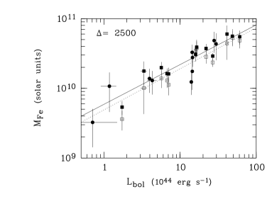
Figure 3: ICM iron mass as a function of the cluster X-ray bolometric luminosity both computed within overdensity $\Delta=2500$ . Filled squares represent CC clusters, whereas filled circles are NCC objects. Open squares show ICM iron mass of CC clusters after subtraction of the iron mass excess. The solid and the dotted lines are the best-fitting power law models (see Table 2) to all clusters taking into account the total ICM iron mass and the iron mass without the iron excess, respectively.

We have investigated the relation between the ICM iron mass and other important observables, i.e. the cluster X-ray bolometric luminosity and temperature. The two correlations for $\Delta=2500$ are shown in Fig. 3 and Fig. 5, respectively. In both figures CC clusters are shown as filled squares, whereas NCC systems are plotted as filled circles. For CC clusters we have also plotted the ICM iron masses without the iron mass excess associated to the cooling regions (open squares in both figures): $M^{\rm noexc}_{\rm Fe}=M_{\rm Fe}-M_{\rm Fe}^{\rm exc}$.

We have characterised the dependence of the physical quantities in the $M_{\rm Fe}-L_{\rm bol}$ and $M_{\rm Fe}-T_{\rm ew}$ relations by means of a linear regression using the algorithm described in Akritas & Bershady (1996, BCES method hereafter), which takes into account measurements errors and intrinsic scatter on the data along both X- and Y-axis. The linear regression has been applied to the logarithms of the physical quantities. In Table 2 we report the best-fit results of the bisector modification of BCES (see Akritas & Bershady 1996 for details). The errors on the best-fit parameters are obtained from 10000 bootstrap resamplings.

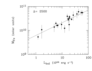
Figure 4: ICM iron mass enclosed within overdensity $\Delta=2500$ plotted as a function of cluster X-ray bolometric luminosity from the catalogue of David et al. (1993). The solid line is the best-fitting power law model (see Table 2).

We find that more luminous clusters posses larger amounts of iron in their ICM. The $M_{\rm Fe}-L_{\rm bol}$ relation, shown in Fig. 3, appears tight, namely the scatter around the best-fitting power law along the y-axis ($M_{\rm Fe}$) is small (see Table 2). The X-ray luminosity and the ICM iron mass are both derived using the emission integral measured from the same BeppoSAX datasets and are therefore subject to some degree of correlation. To test whether the $M_{\rm Fe}-L_{\rm bol}$ relation is affected by systematic effects we have further investigated this relation using bolometric luminosities derived from another totally independent dataset, namely luminosities taken from the work of David et al. (1993) (Fig. 4). We find that the difference between this last correlation and the one measured directly from BeppoSAX data is negligible (see BCES results in Table 2), confirming that the $M_{\rm Fe}-L_{\rm bol}$ relation is robust.

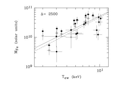
Figure 5: ICM iron mass as a function of the cluster deprojected emission-weighted temperature both computed within overdensity $\Delta=2500$ . Symbols and lines have the same meaning as in Fig. 3.

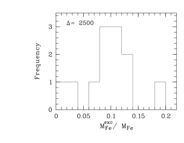
Figure 6: Histogram of the ratio between ICM excess and ICM total iron mass computed at overdensity $\Delta=2500$ for CC clusters.

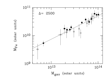
Figure 7: ICM iron mass as a function of ICM gas mass at overdensity 2500. Filled squares and open circles are CC and NCC clusters, respectively. The solid line is the best-fitting power law model to all clusters.

The ICM iron mass also correlates with the deprojected emission-weighted temperature. In Fig. 5 we show that hotter clusters contain larger amounts of iron than cooler systems. Contrary to the $M_{\rm Fe}-L_{\rm bol}$ relation, the $M_{\rm Fe}-T_{\rm ew}$ relation shows a noticeable scatter along the y-axis ($M_{\rm Fe}$), more than a factor 2 larger than that of the $M_{\rm Fe}-L_{\rm bol}$ relation, and shows a clear segregation between CC and NCC clusters. This segregation cannot be entirely due to the contribution of the iron excess observed in CCs to the total amount of iron. Indeed, as shown in Fig. 6, the iron mass excess is a modest fraction of the total ICM iron mass (i.e. only $<20\%$ at overdensity $\Delta=2500$). We hypothesise that the ICM iron mass correlates directly with the cluster luminosity, whereas the correlation between iron mass and temperature is not direct but derives from the combination of the $M_{\rm Fe}-L_{\rm bol}$ relation and the well known relation between X-ray luminosities and gas temperatures (EDM02 and references therein). The $L_{\rm bol}-T_{\rm ew}$ relation (see EDM02 for an extensive discussion about the luminosity-temperature relation derived at various overdensities from the BeppoSAX sample used in this work; and also Markevitch 1998 and references therein for a discussion of the intrinsic scatter in this relation), exhibits a large scatter mostly due to the effect of strong gas cooling in the cores of CC clusters, which are biasing global temperature and luminosity measurements (Fabian et al. 1994). For instance, EDM02 have shown that the scatter in the $L_{\rm bol}-T_{\rm ew}$ relation is reduced by $20\%$ when only CC clusters are considered.

Table 2: Results of the best-fit analysis. To derive the slope of a relation we apply the linear BCES bisector estimator to the logarithm of the power law $Y=aX^{b}$, $\log Y=A+B\log X$ (i.e. $a=10^{A},b=B$; errors are given in parentheses). The emission-weighted temperature, $T_{\rm ew}$, is in units of keV; the luminosity, $L_{\rm bol}$, is in $10^{44}$ erg s^-1; the iron mass, $M_{\rm Fe}$, and the iron mass after subtraction of the iron mass excess (for CC clusters only), $M_{\rm Fe}^{\rm noexc}$, are in $10^{10}M_{\odot}$, the gas mass, $M_{\rm gas}$, is in $10^{13}M_{\odot}$. The scatter on $Y$ is measured as $\left[\sum_{j=1,N}\left(\log Y_{j}-A-B\log X_{j}\right)^{2}/N\right]^{1/2}$ (the scatter along the X-axis can be estimated as $\sigma_{\log X}=\sigma_{\log Y}/B$).

Relation		$\Delta=$2500				$\Delta=$1000
		$A$	$B$	$\sigma_{\log Y}$		$A$	$B$	$\sigma_{\log Y}$
${\rm M_{Fe,10}-L_{bol,44}}$		-0.23 (0.09)	0.57 (0.07)	0.13		-0.23 (0.10)	0.76 (0.07)	0.16
${\rm M_{Fe,10}^{noexc}-L_{bol,44}}$		-0.31 (0.10)	0.59 (0.08)	0.14		-0.34 (0.10)	0.80 (0.08)	0.16
${\rm M_{Fe,10}-L_{bol,44}^{(David\leavevmode\nobreak\ et\leavevmode\nobreak\ al.\leavevmode\nobreak\ 1993)}}$		-0.21 (0.08)	0.53 (0.06)	0.11		-0.01 (0.12)	0.64 (0.09)	0.14
${\rm M_{Fe,10}-L_{44}^{(0.1-2.4\leavevmode\nobreak\ keV)}}$		-0.31 (0.11)	0.67 (0.09)	0.14		-0.07 (0.13)	0.75 (0.10)	0.19
${\rm M_{Fe,10}-T_{ew}}$		-1.10 (0.34)	1.82 (0.40)	0.26		-0.20 (0.71)	1.15 (0.95)	0.37
${\rm M_{Fe,10}^{noexc}-T_{ew}}$		-1.25 (0.31)	1.93 (0.37)	0.24		-0.33 (0.73)	1.25 (0.96)	0.39
${\rm L_{bol,44}-T_{ew}}$		-1.54 (0.51)	3.21 (0.60)	0.39		-0.14 (0.65)	1.78 (0.82)	0.46
${\rm M_{Fe,10}-M_{gas,13}}$		-0.13 (0.04)	0.83 (0.06)	0.10		-0.12 (0.06)	0.88 (0.05)	0.11

To test our hypothesis we have computed the expected parameters and the scatter along the y-axis for the $M_{\rm Fe}-T_{\rm ew}$ relation by combining the best-fitting parameters and scatters of the $M_{\rm Fe}-L_{\rm bol}$ and $L_{\rm bol}-T_{\rm ew}$ relations, and we have compared them with those derived from direct fitting of the $M_{\rm Fe}-T_{\rm ew}$ relation. We find that the parameters computed from the $M_{\rm Fe}-L_{\rm bol}$ and $L_{\rm bol}-T_{\rm ew}$ relations ($A=-1.11,B=1.83$ for $\Delta=2500$), are in good agreement with those derived from direct fitting of the $M_{\rm Fe}-T_{\rm ew}$ relation (see Table 2). Most importantly, we find that the scatter along the y-axis ($M_{\rm Fe}$) observed in the $M_{\rm Fe}-T_{\rm ew}$ relation ($\sigma_{\rm logM_{Fe}}=0.26$) is consistent with the one derived by combining the $M_{\rm Fe}-L_{\rm bol}$ and $L_{\rm bol}-T_{\rm ew}$ relations ($\sigma_{\rm logM_{Fe}}=0.27$). We therefore conclude that the large scatter and the segregation observed in the $M_{\rm Fe}-T_{\rm ew}$ distribution is due to the large dispersion in X-ray luminosities for a given temperature, and that the most direct relation is the one between the ICM iron mass and the X-ray luminosity.

In Fig. 7 we explore the relation between the iron mass and the gas mass in the ICM. Such a relation is expected as a direct consequence of the $M_{\rm Fe}-L_{\rm bol}$ relation since the X-ray luminosity is related to the square of the gas mass ($L_{\rm bol}\propto n_{H}^{2}T^{1/2}$). We find that the iron mass scales linearly with the gas mass (see Table 2), which is equivalent to saying that all nearby clusters have the same iron abundance, $Z_{\rm Fe}\propto M_{\rm Fe}/M_{\rm gas}$. Since the iron in the ICM has been formed in stars this result supports a scenario where the mass in stars in clusters is closely related to the intracluster gas mass. At overdensity $\Delta=2500$ the iron to gas mass ratio, $M_{\rm Fe}/M_{\rm gas}$, ranges between $2.9-9.2\times 10^{-4}$, which corresponds to an iron abundance in solar units of $0.22-0.71$. We note that this measure of the ICM metallicity is not emission-weighted as it is derived from direct integration of the deprojected iron abundance and gas density profiles. This mass-weighted metallicity is $\sim 15\%$ smaller than the emission-weighted projected abundance measured directly from the data within the same overdensity, $\Delta=2500$. The difference is due to the abundance and surface brightness peaks in CC clusters.

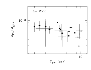
Figure 8: Ratio between ICM iron mass and gas mass, i.e. metallicity, as a function of temperature. Filled squares are CC clusters and open circles are NCC systems. The dotted line is the best-fitting constant model to all clusters.

Finally, as illustrated in Fig. 8 we show that the ratio between the iron and gas mass (at $\Delta=2500$) does not show any trend with the cluster temperature. A constant model fitted over the distribution of all clusters gives a mean metallicity of $0.44\pm 0.02$ ($M_{\rm Fe}/M_{\rm gas}=5.76\pm 0.4\times 10^{-4}$, with $\chi^{2}$/dof=18.2/21). Since CC span a different range in temperature with respect to NCC systems we have fitted the two cluster classes independently: the best-fitting constant for CC clusters is $6.3\pm 0.4\times 10^{-4}$ with $\chi^{2}$/dof=6/11), and that for NCC clusters is $4.5\pm 0.6\times 10^{-4}$ with $\chi^{2}$/dof=5/9), corresponding to iron abundances of $0.51\pm 0.03$ and $0.36\pm 0.05$, respectively. We find that the CC cluster distribution shows a mild negative gradient with increasing temperature: indeed, by performing a fit with a constant plus a linear component we find a statistically modest improvement according to the $F$-test (Prob${}_{\rm F-test}=0.95$).

3.1 The local ICM iron Mass Function and the Metal Content in Clusters

The $M_{\rm Fe}-L_{\rm bol}$ relation allows us to estimate a reliable ICM iron mass once the cluster X-ray luminosity is known. From this relation it is straightforward to derive the iron mass function of the ICM (X$M_{\rm Fe}$F) in the local Universe using the local X-ray luminosity function of clusters (XLF).

We have computed the X$M_{\rm Fe}$F by assuming the XLF of the REFLEX sample (Böhringer et al. 2002, their eq. 4) in the case of an $\Omega_{m}=0.3$ and $\Omega=0.7$ Universe (with parameters of the Schechter function $n_{0}=1.07\times 10^{-7}$ Mpc^-3, $\alpha=1.69\pm 0.045$, $L_{*}=8.36^{+0.9}_{-0.8}10^{44}$ ergs s^-1), and our scaling relation $M_{\rm Fe}-L_{(0.1-2.4\leavevmode\nobreak\ keV)}$ computed with luminosities converted into the 0.1-2.4 keV energy band (parameters A=-0.31, B=0.67, see Table 2). To estimate the clusters contribution to the iron mass budget of the local Universe we have integrated the X$M_{\rm Fe}$F over a given iron mass range. The integral limits have been chosen from the $M_{\rm Fe}-T_{\rm ew}$ relation for a minimum and maximum temperature of 3 and 10 keV, respectively. The resulting iron mass in clusters with respect to the total critical density, $\Omega_{Fe}=\rho_{Fe}/\rho_{c}$, is $4.54\times 10^{-8}$.

From this we have estimated the total metal budget in nearby clusters, by summing over all relevant metals considering a Grevesse & Sauval (1998) solar abundance and assuming that the enrichment is mostly given by SNII (we have assumed metal-to-iron mass ratios accordingly with Nomoto et al. 1997). We compute an upper limit of the metal content in clusters relative to the critical density, $\Omega_{Z}$, of $\sim 1.61\times 10^{-6}$, by excluding only the masses of H and He from the calculation. By excluding the masses of C and N too, as they are both metals not yet measured in the ICM (see Finoguenov et al. 2003), we obtain the lower limit of $\Omega_{Z}\sim 1.47\times 10^{-6}$. This contribution is about a factor 3 smaller than that estimated independently, with different assumption and methods, by Finoguenov et al. (2003).

3.2 The cluster IMLR

The concept of ICM iron mass to light ratio ($M_{\rm Fe}/L_{B}$, IMLR hereafter) as the ratio of the total iron mass in the ICM over the total optical luminosity of galaxies in the cluster was first introduced by Ciotti et al. (1991). This is a fundamental quantity to understand the ICM enrichment (Renzini 1997). Renzini et al. (1993) derived a typical value of the IMLR for rich clusters of $0.01-0.02$ ($M_{\odot}/L_{\odot}$). These values were obtained computing the iron mass in the ICM as the product of the iron abundance times the mass of the ICM gas: $M_{\rm Fe}\propto Z_{\rm Fe}M_{\rm gas}$, using the global cluster value for the abundance, $Z_{\rm Fe}$. Since rich relaxed clusters show abundance gradients, this way of measuring the IMLR tends to overestimate the total amount of iron present in the ICM (see discussion in Sect. 2).

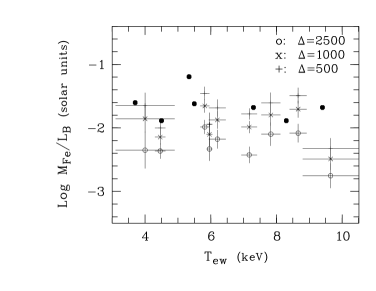
Figure 9: ICM IMLR, $M_{\rm Fe}/L_{\rm B}$, as a function of cluster temperature at $\Delta=2500$ of clusters A1367, A2199, A1795, A426, A85, A2256, A2029, A2142 and A1656 (ordered by increasing temperature). Filled circles are IMLR values taken from Renzini (1997; the 7 cluster in common with our sample), open circles, crosses (x) and crosses (+) are IMLR estimated using iron masses from this work computed within $\Delta=2500$, 1000 and 500, respectively.

We re-compute the IMLR using our ICM iron masses estimated by integrating radially $Z_{\rm Fe}$ with eq. (1). For the 9 clusters with available optical B-band luminosity (we use the same $L_{\rm B}$ used by Renzini 1997 and Arnaud et al. 1992), the mean value of the IMLR at the various overdensities is $5.8\pm 0.9\times 10^{-3}$ ($\Delta=2500$), $1.3\pm 0.2\times 10^{-2}$ ($\Delta=1000$) and $2.0\pm 0.3\times 10^{-2}$ ($\Delta=500$). When the iron mass excess is subtracted from the contribution of the CC clusters the IMLR at overdensity 2500 becomes $5.0\pm 0.7\times 10^{-3}$, therefore this exclusion has a negligible effect.

By comparing our measurements with those of Renzini (1997), we find that their values are in excess of ours by about a factor 2 when using our $\Delta=1000$ values and by about a factor 1.3 when using our $\Delta=500$ values. In a recent review, Renzini (2003), has revised his values by reducing them by $\sim 30\%$, as a consequence of this change his and ours estimates are now in reasonable agreement.

In Fig. 9 we plot our IMLR and those of Renzini (1997) as a function of the cluster temperature. We do not find any dependence of the IMLR with the temperature in agreement with what previously found by Renzini (1997).

4 The iron Mass Excess in Cool Core clusters

NCC clusters have flat abundance profiles, whereas CC clusters have abundance excesses in their cores (Fig. 1). In this Sect. we address the question of assessing the cause of this difference. In our previous work (DM01) we compared the observed abundance excess profiles of four clusters (A2029, A85, A496 and Perseus) with the abundance excess profiles expected when the metal excess distribution traces the light distribution of early-type galaxies of the cluster. We found a good agreement between the observed and expected profiles and, more interestingly, we found that the excess in the expected profiles is entirely due to the light profile of the brightest cluster galaxy (BCG). This indicates that the abundance excess could have been producted by the BCG itself through direct ejection of metal rich gas via SN- or AGN- induced winds. A similar conclusion has been reached by other authors (Fukazawa et al. 2000 and references therein), which suggested that the central galaxy is the cause of the observed abundance peaks. This is furthermore supported by the observational evidence that the X-ray emission peak of CC clusters is always centred on the BCG (e.g. Schombert 1988, Peres et al. 1998, Lazzati & Chincarini 1998).

To explore in greater detail the possibility that the BCG itself is producing the observed iron abundance peak we have estimated the amount of iron that such a galaxy is able to eject during its life performing the exercise reported in the following. We have collected from the literature optical Kron-Cousin $R_{c}$-band magnitudes of the BCGs integrated through an aperture of constant physical radius of $\approx 18$ kpc (Postman & Lauer 1995). For A85, A496, A1795 and A2029 we have converted $r$-gunn magnitudes on the same aperture taken from Hoessel, Gunn & Thuan (1980) into $R_{c}$ magnitudes using the relation $r-Rc=0.37$ given in Fukugita et al. (1995), while optical magnitudes were not available for the central galaxies of 2A 0335$+$096 and PKS 0745$-$191. Typical errors of the adopted magnitudes are less than 0.05 mag, while redshifts of galaxies are given within an error of 0.0002. All the apparent magnitudes have been corrected for the galactic extinction assuming the E(B-V) values given by Burstein and Heiles (1984). Then, the stellar mass content of the BCGs has been derived from their absolute $R_{c}$ magnitudes and from the mass-to-$R_{c}$ band light ratio. The adopted ranges of values of k-corrections and mass-to-light ratios have been calculated using the latest version of the stellar population synthesis code of Bruzual & Charlot (1993), considering two possible models: a Simple Stellar Population (SSP) and an exponentially declining star formation rate with a timescale $\tau$ = 1.0 Gyr. Both population synthesis models have been built assuming a Salpeter Initial Mass Function (IMF) and solar metallicity (Z=0.020), and a typical age of 13 Gyr has been chosen to represent our massive ellipticals. We obtain typical mass-to-light ratios of 8.6 and 7.9 (solar units) for the SSP and $\tau=1.0$ Gyr models respectively (assuming M${}_{\odot,R_{c}}=4.4$, derived from Allen 1973). It is worth noting that the mass in the above ratios includes the total mass of gas involved in the star forming process. Indeed, considering the stellar mass really “locked” into stars (i.e. the difference from the total processed gas and the processed gas returned to the interstellar medium of galaxies) we would obtain $30\%$ lower masses. Variations of the age of the models in the range of 10 - 15 Gyr would produce differences in the corresponding mass-to-light ratios of less than $20\%$ while the major source of uncertainty in the mass estimate of the BCGs stellar content comes from the choice of IMF. Indeed, assuming a Scalo IMF we would obtain stellar masses lower by a factor of 2, while a Miller-Scalo IMF would bring stellar masses down by more than $30\%$ with respect to those obtained with the chosen Salpeter IMF. Given the low redshift of the BCGs in the selected sample, k-corrections are small (i.e., lower than 0.1 mag) and their change due to variations of the models parameters do not affect the final estimate of the stellar masses significantly. Putting everything together the resulting stellar mass content of the BCGs in the selected sample is in the range $\sim 6\times 10^{11}-4\times 10^{12}$ $M_{\odot}$.

We have then converted the stellar mass range into a range of iron masses ejected into the ICM by these galaxies considering the chemical evolution of ellipticals as modelled by Pipino et al. (2002) (we have interpolated the values given in their Table 4). The ejected iron mass range obtained is $\sim 1-5\times 10^{9}$ $M_{\odot}$. It is worth noting that these masses are lower limits to the iron mass ejection since the optical magnitudes within 18 kpc do not take into full account the large stellar halos which are present in many of the BCGs (e.g., Kemp & Meaburn 1991 found a 0.6 Mpc halo in the cD galaxy of A3571).

We have compared this expected iron mass range with the iron mass excess measured in the core of CC clusters (see Sect. 3 and eq. 1). Since the observed values range between $0.5-9.5\times 10^{9}$ $M_{\odot}$ (Table 1) and considering that the estimate is characterised by the uncertainties described above, we conclude that the BCGs are able to produce the observed iron mass excess during their lifetime.

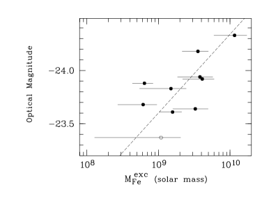
Figure 10: BCG optical magnitude as a function of iron mass excess. Open circle marks the binary cluster A2142. Dashed line is the best-fitting power law excluding A2142.

If we assume that the iron mass excess measured in the core of CC clusters is produced by the BCG alone, then we expect that the properties of the BCGs, more specifically their optical magnitudes, which are a measure of their stellar masses, correlate with the iron mass excess. Indeed this correlation seems to be present in our data as illustrated in Fig. 10. The cluster marked with an open circle in the Fig. is A2142, which has an abundance profile consistent with being flat (DM01): as discussed in DM01 the cause of this flattening is probably physical as A2142 is a known binary system (e.g. a cluster that contains two bright galaxies of similar magnitudes), which experienced a recent merger event that probably influenced the abundance peak in its core (Oegerle, Hill & Fitchett 1995, Buote & Tsai 1996, Henry & Briel 1996, Markevitch et al. 2000). In the rest of this work we will exclude A2142 from our analysis because it is a peculiar cluster that cannot be considered representative of the CC clusters class. Nevertheless, this cluster will be always plotted in the next figures and marked as an open circle.

We find that the optical magnitude and the iron mass excess correlate (the non-parametric correlation coefficients for the 9 BCG with available optical magnitude is 0.67), and, although there is a large scatter in our relation and the statistics is small, we find that the dependence between the two quantities is consistent with being linear (the best-fitting parameters are reported in Table 3). If we assume that the BCG is the sole origin of the iron excess observed in CC’s cores and that the metals ejected by the BCG remain confined in the vicinity of the galaxy, then this relation may imply that the efficiency of the mechanisms that play a role in transporting the metals from the galaxy to the ICM may be roughly the same in all clusters. A larger sample of BCGs in CC clusters and deeper optical photometry, both at optical and NIR wavelengths, are needed to study in greater detail this important relation.

Table 3: Results of the BCES best-fit analysis. The parameters A, B and the scatters $\sigma_{\log X}$, have the same meaning as in Table 2. We have considered here only quantities computed at overdensity 2500. The last column reports Spearman’s Rank-Order correlation coefficient, $\rho$, for a set of physical quantities; in parentheses is reported the probability ($P_{\rho}$) of exceeding its value under null hypothesis of not associated dataset (a small value in probability indicates significant correlation).

Relation	$A$	$B$	$\sigma_{\log Y}$	$\rho(P_{\rho})$
${\rm M_{Fe,9}^{exc}-T_{ew}}$	-1.25 (0.66)	2.23 (0.83)	0.26	0.84 (1e-3)
${\rm M_{opt}-T_{ew}}$	-22.3 (0.67)	-2.04 (0.86)	0.20	-0.72 (0.03)
${\rm M_{opt}-M_{Fe,9}^{exc}}$	-23.6 (0.20)	-0.74 (0.41)	0.22	-0.67 (0.05)

4.1 The Cluster/BCG connection

At the spatial scales examined by BeppoSAX observations CC clusters appear as dynamically relaxed objects. X-ray observations of their central regions show in general simultaneously declining temperature profiles (e.g. Allen et al. 2001), increasing iron abundance profiles and surface brightness excesses with respect to single $\beta$-model profiles (e.g. Mohr et al. 1999). When these properties are present, optical observations always reveal the presence of a BCG located at the bottom of the cluster’s potential well, thus there must be some physical connection between all these observational facts. In this Sect. we try to investigate the physical link between the cluster and the BCG. We expect that the relation between their properties, such as optical magnitude of the galaxy and cluster temperature or iron mass excess, may give us clues on the way clusters and BCGs formed.

A number of theories have been proposed for the formation of the central giant galaxies in clusters. The first models, which are sometimes generically labelled as “galactic cannibalism”, require that a cluster (with its potential well) has already formed and indeed these models predate the advent of the hierarchical scenario for the structure formation. These models have been found to be inadequate to explain the bulge of the BCGs because the dynamical timescales involved are too long to reproduce the observed bulge luminosities of these galaxies (e.g. Tremaine 1990).

Another model requires that the formation of the BCG is significantly influenced by gas accretion and enhanced star formation from a cooling-flow (Fabian 1994). The final fate of the cooling flow gas is to cool down, accreting significantly on the central galaxy, and triggering star formation. This process would require BCGs to have an anomalously blue colours which are not observed (e.g. Andreon et al. 1992, McNamara & O’Connel 1989, 1992). However, recent works based on XMM-Newton (e.g. Peterson et al. 2001, Kaastra et al. 2001, Tamura et al. 2001, Molendi & Pizzolato 2001, David ) and Chandra (e.g. David et al. 2001, Ettori et al. 2002, Blanton, Sarazin & McNamara 2003) observations of clusters have shown that in the core of CC clusters the gas does not cool beyond a minimum temperature of $\sim 1-3$ keV (Fabian et al. 2001). Many authors (Churazov et al. 2002, Kaiser & Binney 2003, Quilis, Bower & Balogh 2001, Ruszkowski & Begelman 2002, Brüggen & Kaiser 2002, Brighenti & Mathews 2002, Ciotti & Ostriker 2001) have suggested that the gas is prevented from cooling by some form of heating. We conclude that cooling flows are no longer a viable alternative to explain the formation of BCG galaxies.

The last and most popular model is galactic merging in the early history of the formation of the cluster. This model predicts that the BCG forms through mergers of several massive galaxies along a filament early in the cluster history (Merritt 1985, Tremaine 1990). Since in the hierarchical scenario smaller structures form earlier than larger structures, a peculiarity of this model is that the formation of the BCG (or at least of its bulge) predates or coincides with the formation of the cluster. Numerical simulations (West 1994, Garijo et al. 1997, Dubinski 1998) favour this picture. In the simulation of Dubinski (1998) galaxy merging naturally produces a massive central galaxy with surface brightness and velocity dispersion profiles very similar to those observed in BCGs; the bulk of the BCG’s luminosity forms early in the cluster’s history, after a rapid merging of the most massive galaxies and further accretion does not change significantly the mass of the galaxy. Other indications supporting the hypothesis of hierarchical assembly of BCGs come from large scale observations, that show that BCGs tend to be aligned with the galaxy and X-ray gas distributions. This tendency continues to cluster scales up to $\sim 20-30$ h^-1 Mpc (Melott, Chambers & Miller 2001) and irregular clusters show a tendency to be more aligned with their neighbours and are preferentially found in high-density environments (Plionis & Basilakos 2002). Furthermore, BCGs are often very flat and their flattening is not primarily due to rotation indicating that they probably form with a triaxial structure. A natural explanation for this behaviour can be given in the context of aspherical accretion from filaments.

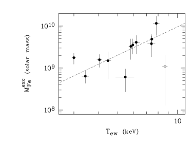
Figure 11: Iron mass excess in cool core clusters plotted as a function of the cluster temperature at overdensity 2500. Open circle marks binary cluster A2142. The dashed line is the BCES best-fitting power law computed excluding A2142.

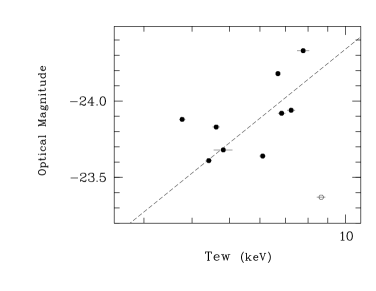
Figure 12: BCG optical magnitude as a function of cluster temperature at overdensity 2500. Open circle marks the binary cluster A2142. Dashed line is the best-fitting power law excluding A2142.

The BeppoSAX data show that the iron mass excess correlates with the cluster temperature (at $\Delta=2500$) (Fig. 11). The best-fitting parameters obtained using our eleven CC clusters (A2142 is excluded, see discussion in Sect. 4), are reported in Table 3. Since the temperature is related to the cluster gravitational mass ($M_{\rm tot}\propto T^{3/2}$), a possible explanation of the observed correlation is that more massive clusters contain more massive BCGs, which are producing larger quantities of iron through feedback mechanisms during their life. If this picture is correct than we expect that the optical luminosities of the BCGs correlate both with the cluster temperatures and the iron mass excesses. We have already shown in the previous Sect. (see Fig.10), that the optical magnitude of the BCG correlates with the iron mass excess. The other expected correlation, $M_{\rm opt}-T_{\rm ew}$, is plotted in Fig. 12. The non-parametric correlation coefficients for the 9 BCGs with available optical magnitude is 0.72 (Prob=0.03), indicating the two quantities correlate. The best-fit to our data (A2142 excluded) is given in Table 3. This correlation implies that the BCG formation is closely related to that of the whole cluster and that subsequent mergers with other cluster galaxies and other accretions events with smaller clusters or groups produce little change in its overall properties, or at least of its bulge, if this where not the case than the properties of the BCGs would depend on the different mass aggregation history of each cluster and we would not observe the correlations reported in Fig. 10, Fig. 11 and Fig. 12. A positive correlation between the optical magnitude of the BCG and the hot gas temperature of its host cluster, $M_{\rm opt}-T_{\rm ew}$, has also been found by other authors (Edge & Steward 1991, Edge 1991, Katayama et al. 2003), using larger samples of BCGs.

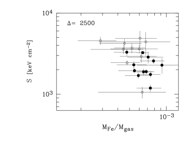
Figure 13: Entropy versus iron abundance expressed in the form $M_{\rm Fe}/M_{\rm gas}$ for CC (filled circles) and NCC (open circles) clusters. Both quantities are computed at overdensity 2500.

As discussed above, the scenario where the properties of the central giant galaxy are related to those of the hosting cluster is expected in the hierarchical formation of the structures. In a recent work based on hydrodynamic simulations of large-scale structure formation including radiative cooling, Motl et al. (2003) suggest that cool cores in rich clusters form and grow in mass predominantly from hierarchical assembly of discrete subclusters, that contain pre-cooled gas and low temperature and entropy cores, and that flow into the clusters along the network filaments. Given the larger ages of these accreting subclumps and the presence of a high fraction of condensed cool gas, it is reasonable to assume that enrichment processes through star formation feedback had time to take place before accretion. An indications that the gas in the accreting sub-clumps is already enriched before cluster relaxation may come from X-ray observations of BCGs in binary clusters (i.e. clusters with two BCGs). The Coma cluster can be considered the prototype of a binary clusters, hosting two dominant galaxies (NGC 4889 and NCG 4874). Vikhlinin et al. (2001) analysing a Chandra observation of these two galaxies found that both BCGs are able to retain part of their ISM and that both ISM have mean abundances larger than that of the surrounding hotter ICM. The analysis of XMM-Newton EPIC data confirms the Chandra results (Molendi private communication). In the hierarchical model we expect that during the relaxation process of the Coma cluster the two BCGs will eventually merge into a unique massive galaxy with an associated abundance peak and a cool core. In this model it is natural to expect cool core clusters to also show abundance excesses in their cores as the results of the accretion process. In other words we expect regions with lower entropy (with the entropy defined as $S=kT_{e}/n^{2/3}_{e}$ keV cm^-2) to be also characterised by higher metal abundances. This is actually the case as shown in Fig. 13, where the entropy measured at overdensity $\Delta=2500$ (about $1/3-1/4$ of the virial radius) are plotted as a function of the iron abundances measured at the same overdensity for both CC and NCC clusters. We find that CC clusters tend to populate a different region of the entropy-abundance plane with respect to NCC clusters, namely a region where lower entropy values correspond to higher abundances.

5 Summary

In this paper we have derived ICM iron masses for a sample of 22 nearby rich cluster of galaxies, observed with BeppoSAX, by directly integrating the deprojected iron abundance and gas density profiles. In the first part of the paper we have discussed the global metal content of our cluster sample while in the second we have concentrated on the iron mass associated to the abundance excess found in CC clusters. Our main results for the first part are as follows.

1. The deprojected abundance profiles are strongly peaked for CC clusters while they remain constant for NCC systems in agreement with what previously found for the projected profiles published in DM01.

2. The relationship between ICM iron mass and other fundamental quantities is through the gas mass. Since the iron in the ICM has been formed in stars our result supports a scenario where the mass in stars in clusters is closely related to the ICM gas mass.

3. We have used the ICM iron mass vs. X-ray cluster luminosity scaling law, and the local X-ray luminosity function, to derive the iron mass function for the local universe. By integrating this function, we have derived the iron and total metal contribution of local clusters to the metal budget of the universe, $\Omega_{\rm Fe}$ and $\Omega_{Z}$, finding them to be $\sim 4.5\times 10^{-8}$ and $\sim 1.5\times 10^{-6}$, respectively.

4. The mean IMLR computed at various overdensities for the 9 clusters in our sample with available optical luminosities range between $5.8\pm 0.9\times 10^{-3}$ at $\Delta=2500$ and $2.0\pm 0.3\times 10^{-2}$ at $\Delta=500$. These values are consistent with the revised values published by Renzini (2003).

Our main results for the second part are as follows.

1. The iron mass associated to abundance excess in CC clusters is of $\sim 0.5-9.5\times 10^{9}M_{\odot}$, this is about $10\%$ of the total ICM iron mass (at $\Delta=2500$). Using population synthesis models to estimate the BCG stellar mass from its observed $R_{c}$ magnitude and chemical enrichment models to derive the iron mass ejected into the ICM from the stellar mass, we find that the BCG is able to produce the iron mass excess observed in CC clusters during its life.

2. We find that the optical light of the BCG correlates with both the cluster temperature and the iron mass excess, implying that there is a strong correlation between the galaxy and the cluster potential well. This result favours current hierarchical formation scenarios of structures where the BCG is assembled at the beginning of the cluster formation process from pre-enriched subclumps.

In conclusion we would like to stress that more detailed optical observations are needed to derive the luminosity of the cluster and of the central galaxy (bulge and halo), near IR observations would be particularly useful as the probe of their giant old stellar population responsible for the bulk of the enrichment. At the same time deeper X-ray XMM-Newton (for external and intermediate regions) and Chandra (for the innermost regions) observations are required to map in greater detail metal abundances in clusters.

- (1) Allen C. W., 1973, Astrophysical Quantities, Athlon Press, London
- (2) Allen, S. W., Schmidt, R. W. & Fabian, A. C. 2001, MNRAS, 328L, 37
- (3) Allen, S. W. & Fabian, A. C. 1998, MNRAS, 297L, 63
- (4) Akritas, M. G. & Bershady, M. A. 1996, ApJ, 470, 706
- (5) Anders, E. & Grevesse, N. 1989, GeCoA, 53, 197
- (6) Andreon, S., Garilli, B., Maccagni, D., Gregorini, L. & Vettolani, G. 1992, A&A, 266, 127
- (7) Arnaud, M., Rothenflug, R., Boulade, O., Vogroux, L., Vangioni-Flam, E. 1992, A&A, 254, 49
- (8) Blanton, E. L., Sarazin, C. L., McNamara, B. R. 2003, ApJ, 585, 227
- (9) Boehringer, H. et al. 2002, ApJ, 566, 93
- (10) Brighenti, F. & Mathews, W. G. 1999, ApJ, 515, 542
- (11) Bruzual, A. G. & Charlot, S. 1993, ApJ, 405, 538
- (12) Buote, D. A., & Tsai, J. C. 1996, ApJ, 458, 27
- (13) Burstein, D. & Heiles, C. 1984, ApJS, 54, 33
- (14) Ciotti, L. & Ostriker, J. P. 2001, ApJ, 551, 131
- (15) Ciotti, L., Pellegrini, S., Renzini, A., D’Ercole, A. 1991, ApJ, 376, 380
- (16) David, L.P., Slyz, A., Jones, C., Forman, W., Vrtilek, S. D., Arnaud, K. A. 1993, ApJ, 412, 479
- (17) De Grandi, S. & Molendi, S. 2002, ApJ, 567, 163
- (18) De Grandi, S. & Molendi, S. 2001, ApJ, 551, 153 (DM01)
- (19) Della Ceca, R., Scaramella, R., Gioia, I.M., Rosati, P., Fiore, F., Squires, G. 2000, A&A, 353, 498
- (20) Dubinski, J. 1998, ApJ, 502, 141
- (21) Dupke, R. A. & White, R. E. III 2000, ApJ, 537, 123
- (22) Edge, A. C. 1991, MNRAS, 250, 103
- (23) Edge, A. C. & Stewart, G. C. 1991, MNRAS, 252, 428
- (24) Ettori, S., Allen, S. W. & Fabian, A. C. 2001, MNRAS, 322, 187
- (25) Ettori, S., De Grandi, S. & Molendi, S. 2002, A&A, 391, 841 (EDM02)
- (26) Ettori, S., Fabian, A. C., Allen, S. W., Johnstone, R. M. 2002, MNRAS, 331, 635
- (27) Fabian, A. C. 1994, ARA&A, 32, 277
- (28) Fabian, A. C., Crawford, C. S., Edge, A. C., Mushotzky, R. F. 1994, MNRAS, 267, 779
- (29) Finoguenov, A., Arnaud, M. & David, L. P. 2001, ApJ, 555, 191
- (30) Finoguenov, A., Matsushita, K., Boehringer, H., Ikebe, Y. & Arnaud, M. 2002, A&A, 381, 21
- (31) Finoguenov, A., Burkert, A. & Boehringer, H. 2003, ApJ, in press (astro-ph/0305190)
- (32) Fujita, Y. & Takahara, F. 1999, ApJ, 519L, 51
- (33) Fukazawa, Y., Makishima, K., Tamura, T., Ezawa, H., Xu, H., Ikebe, Y., Kikuchi, K., Ohashi, T. 1998, PASJ, 50, 187
- (34) Fukazawa, Y., Makishima, K., Tamura, T., Nakazawa, K., Ezawa, H., Ikebe, Y., Kikuchi, K., Ohashi, T. 2000, MNRAS, 313, 21
- (35) Fukugita, M., Shimasaku, K. & Ichikawa, T. 1995, PASP, 107, 945
- (36) Garijo, A., Athanassoula, E. & Garcia-Gomez, C. 1997, A&A, 327, 930
- (37) Gastaldello, F. & Molendi, S. 2002, ApJ, 572, 160
- (38) Gnedin, N. Y. 1998, MNRAS, 294, 407
- (39) Grevesse, N. & Sauval, A. J. 1998, SSRv, 85, 161
- (40) Gunn, J. E. & Gott, J. R. III 1972, ApJ, 176, 1
- (41) Henry, J. P., & Briel, U. G. 1996, ApJ, 472, 137
- (42) Hicks, A. K., Wise, M. W., Houck, J. C., Canizares, C. R. 2002, ApJ, 580, 763
- (43) Hoessel, J. G. Gunn, J. E. & Thuan, T. X. 1980, ApJ, 241, 486
- (44) Irwin, J. A., & Bregman J. N. 2001, ApJ, 546, 150
- (45) Katayama, H., Hayashida, K., Takahara, F. & Fujita, Y. 2003, ApJ, 585, 687
- (46) Kauffmann, G. & Charlot, S. 1998, MNRAS, 294, 705
- (47) Kemp, S. N. & Meaburn, J. 1991, MNRAS, 252P, 27
- (48) Lazzati, D. & Chincarini, G. 1998, A&A, 339, 52
- (49) Lin, Y-T, Mohr, J. J., Stanford, S. A. 2003, ApJ, 591, 749
- (50) Makishima, K., Ezawa, H. Fukazawa, H., Honda, H., et al. 2001, PASJ, 53, 401
- (51) Matsushita, K., Finoguenov, A., Boehringer, H. 2003, A&A, 401, 443
- (52) Markevitch, M. 1998, ApJ, 504, 27
- (53) Markevitch, M., et al. 2000, ApJ, 541, 542
- (54) McNamara, B. R. & O’Connell, R. W. 1989, ApJ, 98, 2018
- (55) McNamara, B. R. & O’Connell, R. W. 1992, ApJ, 393, 579
- (56) Melott, A. L., Chambers, S. W. & Miller, C. J. 2001, 559L, 75
- (57) Merritt, D. 1985, ApJ, 289, 18
- (58) Mohr, J. J., Mathiensen, B., & Evrard, A. E. 1999, ApJ, 517, 627
- (59) Molendi, S. & Gastaldello, F. 2001, A&A, 375L, 14
- (60) Motl, P. M., Burns, J. O., Loken, C., Norman, M. L. & Bryan, G. 2003, ApJ, in press (astro-ph/0302427)
- (61) Mushotzky, R. F. & Loewenstein, M. 1997, ApJ, 481L, 63
- (62) Oegerle, W. R., Hill, J. M., & Fitchett, M. J. 1995, AJ, 110, 32
- (63) Peres, C. B., Fabian, A. C., Edge, A. C., Allen, S. W., Johnstone, R. M. 1998, MNRAS, 298, 416
- (64) Pipino, A., Matteucci, F., Borgani, S. & Biviano, A. 2002, NewA, 7, 227
- (65) Plionis, M. & Basilakos, S. 2002, MNRAS, 329L, 47
- (66) Postman, M. & Lauer, T. R. 1995, ApJ, 440, 28
- (67) Pratt, G. W. & Arnaud, M. 2002, A&A, 394, 375
- (68) Press, W. H., Teuklosky, S. A., Vetterling, W. T. & Flannery, B. P. 1992, Numerical Recipes (Cambridge University Press)
- (69) Renzini, A. 1997, ApJ, 488, 35
- (70) Renzini, A. 2003, in Carnegie Obs. Astrophys. Series, Vol. 3, Clusters of Galaxies: Probes of Cosmological Structure and Galaxy Evolution, ed. J. S. Mulcaey, A. Dressler, and A. Oemler (Cambridge: Cambridge Univ. Press), astro-ph/0307146
- (71) Renzini, A., Ciotti, L., D’Ercole, A., Pellegrini, S. 1993, ApJ, 419, 52
- (72) Schmidt, R. W., Fabian, A. C. & Sanders 2002, MNRAS, 337, 71
- (73) Schombert, J. M. 1998, ApJ, 328, 475
- (74) Tremaine, S. 1990, in Dynamics and Interactions of Galaxies, ed. R. Wielen (Berlin, New York: Springer), 394
- (75) Toniazzo, T. & Schindler, S. 2001, MNRAS, 325, 509
- (76) Tozzi, P., Rosati, P., Ettori, S., Borgani, S., Mainieri, V., Norman, C. 2003, ApJ, in press (astro-ph/0305223)
- (77) Vikhlinin, A., Markevitch, M., Forman, W. & Jones, C. 2001, ApJ, 555L, 87
- (78) West, M. J. 1994, MNRAS, 268, 79