Density field in extended Lagrangian perturbation theory

Abstract

We analyzed the performance of a perturbation theory for nonlinear cosmological dynamics, based on the Lagrangian description of hydrodynamics. In our previous paper, we solved hydrodynamic equations for a self-gravitating fluid with pressure, given by a polytropic equation of state, using a perturbation method. Then we obtained the first-order solutions in generic background universes and the second-order solutions for a wider range of polytrope exponents. Using these results, we describe density fields with scale-free spectrum, SCDM, and LCDM models. Then we analyze cross-correlation coefficient of the density field between N-body simulation and Lagrangian linear perturbation theory, and the probability distribution of density fluctuation. From our analyses, for scale-free spectrum models, the case of the polytrope exponent $5/3$ shows better performance than the Zel’dovich approximation and the truncated Zel’dovich approximation in a quasi-nonlinear regime. On the other hand, for SCDM and LCDM models, improvement by the effect of the velocity dispersion was small.

I Introduction

The Lagrangian approximation for structure formation in cosmological fluids provides a relatively accurate model even in quasi-linear regime, where density fluctuation becomes unity. The Zel’dovich approximation (hereafter ZA) zel ; buchert92 ; coles ; saco , a linear Lagrangian approximation for dust fluid, describes the evolution of density fluctuation better than Eulerian approximation munshi ; sahsha . Although ZA gives an accurate description until quasi-linear regime develops, ZA cannot describe the model after the formation of caustics. In ZA, even after the formation of caustics, the fluid elements keeps moving in the direction set up by the initial condition. ZA cannot describe compact and high density structures such as pancakes, skeletons, or clumps, while N-body simulation shows the presence of clumps with a very wide range in mass at any given time davis . In general, after the formation of caustics, hydrodynamical description becomes invalid.

In order to proceed with a hydrodynamical description without the formation of caustics, the qualitative pressure gradient zel82 and thermal velocity scatter kotok ; shandarin in a collisionless medium had been discussed. After that, the ‘adhesion approximation’ gurbatov was proposed from the consideration of nonlinear wave equations like Burgers’ equation. In the ‘adhesion approximation’, an artificial viscosity term is added to ZA. As another modification, a Gaussian cutoff is applied to the initial power spectrum of density fluctuation and then evolves with the ZA. This modified approximation is called the ‘Truncated Zel’dovich approximation’ (hereafter TZA)  cms ; mps . These modified approximations successfully avoid the formation of caustics and describe the evolution for long time. However, the physical origin of the modification is not clarified.

We reconsider the basic, fundamental equation for the motion of matter. The collisionless Boltzmann equation BT describes the motion of matter in phase space. The basic equations of hydrodynamics are obtained by integrating the collisionless Boltzmann equation over velocity space. In past approximations, such as ZA and its modified version, velocity dispersion was ignored. Buchert and Domínguez budo argued that the effect of velocity dispersion become important beyond the caustics. They also argued that models for large-scale structure should rather be constructed for a flow which describes the average motion of a multi-stream system. Then they showed that when the velocity dispersion is still small and can be considered isotropic, that gives effective ’pressure’ or viscosity terms. Furthermore, they argued the relation between mass density $\rho$ and pressure $P$, i.e. an ‘equation of state’. If the relation between the density of matter and pressure seems barotropic, the equation of state should take the form $P\propto\rho^{5/3}$. Buchert et al. bdp showed how the viscosity term is generated by the effective pressure of a fluid under the assumption that the peculiar acceleration is parallel to the peculiar velocity; Domínguez domi00 ; domi0106 clarified that a hydrodynamic formulation is obtained via a spatial coarse graining in a many-body gravitating system, and the viscosity term in the ‘adhesion approximation’ can be derived by the expansion of coarse-grained equations.

Domínguez domi0103 also reported on a study of the spatially coarse-grained velocity dispersion in cosmological N-body simulations. The analysis showed that polytrope exponent becomes $\gamma\simeq 5/3$ in a quasi-nonlinear regime, and $\gamma\simeq 2$ in a strongly nonlinear regime. Domínguez and Melott dome0310 discussed polytrope exponents of velocity dispersion in N-body simulations. According to their results, the exponents depend on a model of initial density fluctuation.

From these points, the extension of Lagrangian perturbation theory to cosmological fluids with pressure has been considered. Actually, Adler and Buchert adler have formulated the Lagrangian perturbation theory for a barotropic fluid. Morita and Tatekawa moritate and Tatekawa et al. tate02 solved the Lagrangian perturbation equations for a polytropic fluid up to second order for cases where the equations are solved easily. Hereafter, we call this model the ‘pressure model’.

In this paper, we analyze the density field which is described by the Lagrangian approximations; ZA, TZA, and first-order pressure model solutions. We calculate the cross-correlation function of density field between the Lagrangian approximation and N-body simulation. Furthermore we analyze the probability distribution function of density fluctuation for confirmation. From these results, we determine a polytrope exponent in the equation of state. From our analyses of the cross-correlation coefficient and probability distribution function of density fluctuation, we find that the value of the polytrope exponent seems to be $5/3$ for quasi-nonlinear evolution, as Buchert and Domínguez argued budo . However, for the determination of a proportion fixed number in equation of state, we must consider further physical processes or carry out high-resolutional N-body simulation.

This paper is organized as follows. In Sec. II, we present Lagrangian perturbative solutions: In Sec. II.1, we show the first-order solution of pressure model in the Einstein-de Sitter background. For comparison, in Sec. II.2 and II.3, we show the solution of ZA and the procedure of TZA.

In Sec. III, we compare the density field between the Lagrangian approximations and N-body simulation. In Sec.III.1, we calculate the cross-correlation coefficient of the density field. Though it seems that we can reach a conclusion in this analysis, it is insufficient. Therefore in Sec. III.2, we analyze the probability distribution function of density fluctuation. In Sec. IV, we discuss our results and state conclusions.

II Lagrangian approximations in gravitational instability theory

II.1 First-order solutions of the pressure model

In this section, we present perturbative solutions in the Lagrangian description. The matter model we consider is a self-gravitating fluid with mass density $\rho$ and ‘pressure’ $P$, which is given by the presence of velocity dispersion. The ‘pressure’ we adopt here is the same as was introduced by Buchert and Domínguez budo , i.e. the diagonal component of the velocity dispersion tensor when the velocity dispersion is assumed to be isotropic in the Jeans equation BT . In Lagrangian hydrodynamics, the comoving coordinates $\bm{x}$ of the fluid elements are represented in terms of Lagrangian coordinates $\bm{q}$ as

$$\bm{x}=\bm{q}+\bm{s}(\bm{q},t)\,,$$ (1)

where $\bm{q}$ are defined as initial values of $\bm{x}$, and $\bm{s}$ denotes the Lagrangian displacement vector due to the presence of inhomogeneities. From the Jacobian of the coordinate transformation from $\bm{x}$ to $\bm{q}$, $J\equiv\det(\partial x_{i}/\partial q_{j})=\det(\delta_{ij}+\partial s_{i}/\partial q_{j})$, the mass density is given exactly as

$$\rho=\rho_{\rm b}J^{-1}\,.$$ (2)

We decompose $\bm{s}$ into the longitudinal and the transverse modes as $\bm{s}=\nabla_{\bm{q}}S+\bm{S}^{\rm T}$ with $\nabla_{\bm{q}}\cdot\bm{S}^{\rm T}=0$. In this paper, we show an explicit form of perturbative solutions in only Einstein-de Sitter universe. For a generic background universe, we obtained the perturbation solutions in our previous paper tate02 .

The transverse modes can be solved easily. The first-order solutions become as follows:

$$\bm{S}^{\rm T}\propto a^{0},\;a^{-1/2}\,.$$ (3)

Because the solutions do not depend on ’pressure’, the solutions of this mode in ZA become the same in form. The transverse modes do not have a growing solution in a first-order approximation.

For the longitudinal modes, we carry out Fourier transformation with respect to the Lagrangian coordinates $\bm{q}$. If we assume a polytropic equation of state $P=\kappa\rho^{\gamma}$ with a constant $\kappa$ and a polytrope exponent $\gamma$, we can write an explicit form of first-order perturbative solutions. In the Einstein-de Sitter background, the solutions are written in a relatively simple form. They are, for $\gamma\neq 4/3$,

$$\widehat{S}(\bm{K},a)\propto a^{-1/4}\,\mathcal{J}_{\pm 5/(8-6\gamma)}\left(\sqrt{\frac{2C_{2}}{C_{1}}}\frac{|\bm{K}|}{|4-3\gamma|}\,a^{(4-3\gamma)/2}\right)\,,$$ (4)

where $\mathcal{J}_{\nu}$ denotes the Bessel function of order $\nu$, and for $\gamma=4/3$,

$$\widehat{S}(\bm{K},a)\propto a^{-1/4\pm\sqrt{25/16-C_{2}|\bm{K}|^{2}/2C_{1}}}\,,$$ (5)

where $C_{1}\equiv 4\pi G\rho_{\rm b}(a_{\rm in})\,a_{\rm in}^{\ 3}/3$ and $C_{2}\equiv\kappa\gamma\rho_{\rm b}(a_{\rm in})^{\gamma-1}\,a_{\rm in}^{\ 3(\gamma-1)}$. $\rho_{b}$ and $\bm{K}$ mean background mass density and Lagrangian wavenumber, respectively. $a_{\rm in}$ means scale factor when an initial condition was given.

Here we notice the relation between the behaviors of the above solutions and the Jeans wavenumber, which is defined as

$$K_{\rm J}\equiv\left(\frac{4\pi G\rho_{\rm b}a^{2}}{{\rm d}P/{\rm d}\rho(\rho_{\rm b})}\right)^{1/2}\,.$$

The Jeans wavenumber, which gives a criterion for whether a density perturbation with a wavenumber will grow or decay with oscillation, depends on time in general. If the polytropic equation of state $P=\kappa\rho^{\gamma}$ is assumed,

$$K_{\rm J}=\sqrt{\frac{3C_{1}}{C_{2}}}\,a^{(3\gamma-4)/2}\,.$$ (6)

Equation (6) implies that, if $\gamma<4/3$, $K_{\rm J}$ will be decreased and density perturbations with any scale will decay and disappear in evolution, and if $\gamma>4/3$, all density perturbations will grow to collapse. We rewrite the first-order solution Equation (4) with the Jeans wavenumber:

$$\widehat{S}(\bm{K},a)\propto a^{-1/4}\,\mathcal{J}_{\pm 5/(8-6\gamma)}\left(\frac{\sqrt{6}}{|4-3\gamma|}\frac{|\bm{K}|}{K_{\rm J}}\right)\,.$$ (7)

II.2 Zel’dovich approximation

ZA was obtained as first-order solutions with dust fluid in Lagrangian description zel . The solutions are obtained from the solutions of the pressure model as a limit of weak pressure. For example, in E-dS model, when we take a limit $\kappa\rightarrow 0$ in Equations (4) and (5), the solutions converge to those of ZA:

$$\widehat{S}(\bm{K},a)\propto a,\;a^{-3/2}\,.$$ (8)

ZA is known as perturbative solutions which describe the structure well in quasi-linear scale. However if the caustics appear, the solutions no longer have physical meaning.

II.3 Truncated Zel’dovich approximation

During evolution, the small scale structure contracts and forms caustics. Therefore if we introduce some cutoff in the small scale, we will be able to avoid the formation of caustics cms ; mps . In TZA, for the avoidance of caustics, we introduce a Gaussian cutoff to the initial density spectrum as follows:

$${\cal P}(k,t_{\rm in})\rightarrow{\cal P}(k,t_{\rm in})\exp\left(-k^{2}/k_{NL}\right)\,,$$ (9)

where $k_{NL}$ means ‘nonlinear wavenumber’, defined by

$$1=a(t)^{2}\int_{k_{0}}^{k_{NL}}{\cal P}(k,t_{\rm in})dk\,.$$ (10)

The ‘nonlinear wavenumber’ depends on the scale factor. The relation between the Jeans wavenumber $K_{J}$ and the nonlinear wavenumber $k_{NL}$ will be discussed in Sec. IV.

III Comparison between N-body simulation and Lagrangian approximations

In this section, we show a comparison between N-body simulation and Lagrangian approximations with two statistical quantities. In our previous paper tate02 , we showed that the effect of second order perturbation was still small just before shell-crossing. Therefore we consider only first order perturbation.

We analyze ZA zel , TZA cms ; mps , and the pressure model adler ; moritate ; tate02 . We establish the value of scale factor at $z=0$ with $a=1$. For the initial condition, we set the Gaussian density field with scale-free spectrum;

$$\mathcal{P}(k)\propto k^{n}(n=-1,0,1)\,,$$ (11)

SCDM, and LCDM model. The initial condition was produced by COSMICS COSMICS .

For N-body simulation, we execute $P^{3}M$ code. The parameters of simulation were given as follows:

Number of particles $$: N=64^{3},N=128^{3}\mbox{(Figure~{}\ref{fig:Cor-k1-N128} only)}\,,$$

Box size $$: L=64h^{-1}\mbox{Mpc}\,,$$

Softening Length $$: \varepsilon=0.05h^{-1}\mbox{Mpc}\,,$$

Course-Graining Length $$: l=1,2,4h^{-1}\mbox{Mpc}\,,$$

Hubble patameter $$: h=0.71\,.$$

For CDM models, we choose cosmological parameters as follows:

SCDM $$: \Omega_{m}=1.0,\;\Omega_{\Lambda}=0.0,\;\sigma_{8}=0.84$$

LCDM $$: \Omega_{m}=0.27,\;\Omega_{\Lambda}=0.73,\;\sigma_{8}=0.84$$

In the pressure model, we choose a polytrope exponent $\gamma=4/3,5/3$: In the case of $\gamma=4/3$, we obtain the simplest perturbative solution given by Equation (5) that is described by the power-law of the time variable. $\gamma=5/3$ is given from theoretical argumentation by Buchert and Domínguez budo . They argued kinematic considerations using collisionless Boltzmann equation and derived $\gamma=5/3$. The exponent is equivalent to the adiabatic process of an ideal gas. Because we cannot decide on a proportional constant $\kappa$ in the equation of state from past discussion, we choose several values. In this paper, instead of $\kappa$, we write an initial ($a=10^{-3}$, i.e. $z=1000$) Jeans wavenumber, given by Equation (6).

Here we show how we set up the initial condition in the pressure model. We adjust the initial condition in the pressure model to be the same as that in ZA: the initial peculiar velocity in the pressure model is same as that in ZA. The procedure for setting up initial condition was shown in our previous papers moritate ; tate02 .

III.1 Cross-correlation coefficient

First we calculate the cross-correlation coefficient of density fields. The Cross-correlation coefficient was used for the comparison of the resulting density fields  cms ; mps ; msw ; Buchert94 ; Melott95 ; Karakatsanis97 . The cross-correlation coefficient is defined by

$$S\equiv\left<\frac{\delta_{1}\delta_{2}}{\sigma_{1}\sigma_{2}}\right>\,,$$ (12)

where $\sigma_{i}$ means the density dispersion of model $i$,

$$\sigma_{i}\equiv\sqrt{\left<\delta_{i}^{2}\right>}.$$ (13)

$S=1$ means that the pattern of density field of two models coincide with each other. In linear regime, the density dispersion remains $\sigma\ll 1$. Although we develop the structure until it becomes strongly nonlinear regime ($\sigma_{N-body}>1$), we especially analyze it in the quasi-nonlinear regime ($\sigma_{N-body}\simeq 1$).

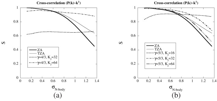
Figure 1: The cross-correlation coefficient of density fields between the N-body simulation and Lagrangian approximations. Primordial density fluctuation is given by the scale-free spectrum $P(k)\propto k^{1}$ ($N=64^{3},l=1h^{-1}\mbox{Mpc}$).  (a) When we choose $\gamma=4/3$, the function deviates from that of ZA in linear regime. (b) In the case of $\gamma=5/3$, we can obtain a better result than TZA.

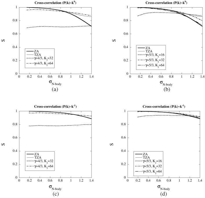
Figure 2: The cross-correlation coefficient of density fields between the N-body simulation and Lagrangian approximations ($N=64^{3},l=1h^{-1}\mbox{Mpc}$, scale-free spectrum model).  (a) $P(k)\propto k^{0}$. The case of $\gamma=4/3$.  (b) $P(k)\propto k^{0}$, the case of $\gamma=5/3$.  (c) $P(k)\propto k^{-1}$. In this model, the difference in the coefficient between ZA and TZA becomes small. The case of $\gamma=4/3$.  (d) $P(k)\propto k^{-1}$, the case of $\gamma=5/3$.

Figure 1-6 shows a comparison of N-body density fields with those predicted by various Lagrangian approximations. First, we notice scale-free spectrum cases (Figure 1-3). As in the past analyses, TZA shows better performance than ZA. Our analyses also show similar tendency, i.e. our analyses do not contradict past analyses.

In the pressure model, the performance strongly depends on the polytrope exponent $\gamma$ and Jeans wavenumber. In the case of $\gamma=4/3$, when we set the initial Jeans wavenumber to be small, even if in linear regime, the approximation deviates from an N-body simulation. Only for the case of $K_{J}=64$ the approximation shows better performance than ZA in a quasi-nonlinear regime. We notice that the result strongly depends on the Jeans wavenumber in the case of $\gamma=4/3$: When we slightly change the value of the Jeans wavenumber, the cross-correlation coefficient changes dramatically. In the case of $\gamma=5/3$, although the result depends slightly on initial Jeans wavenumber, the pressure model shows a better performance than ZA in a quasi-nonlinear regime. Furthermore, the pressure model also shows a better performance than TZA. However, when we consider scale-free spectrum models, the model does not have typical physical scale: the model has only box size, grid size, and softening length. The trend of the result was unchanged when we changed the box size of the model and the softening parameter. When we change the number of particles, the result changes. From a comparison of Figure 1 and Figure 3, we can notice that the results depend on the ratio of grid size and initial Jeans wavenumber. In our calculation, we found out that it was good to set up the value of $\kappa$ so that the initial ($z=1000$) Jeans wavenumber $K_{J}$ was $N^{1/3}/4\leq K_{J}\leq N^{1/3}$. For example, in the case of $N=64^{3}$, as we see in Figure 1 and 2, it is good to choose the initial Jeans wavenumber $16\leq K_{J}\leq 64$.

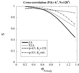
Figure 3: The cross-correlation coefficient of density fields between N-body simulation and Lagrangian approximations. Primordial density fluctuation is given by scale-free spectrum $P(k)\propto k^{1}$ ($N=128^{3},l=1h^{-1}\mbox{Mpc}$). From comparison between Figure 1 and this graph, we can notice that the results depend on the ratio of grid size and initial Jeans wavenumber.

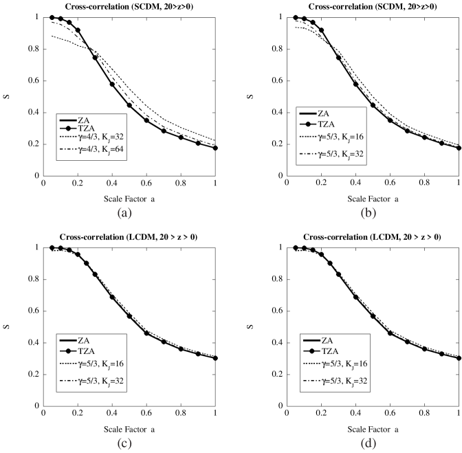
Figure 4: The cross-correlation coefficient of density fields between an N-body simulation and Lagrangian approximations. The primordial density fluctuation is given by the CDM spectrum ($N=64^{3},l=1h^{-1}\mbox{Mpc}$). The model in which hardly a difference appears in is excluded from the graph.  (a) The SCDM model with $\gamma=4/3$.  (b) The SCDM model with $\gamma=5/3$.  (c) The LCDM model with $\gamma=4/3$.  (d) The LCDM model with $\gamma=5/3$.

Next we consider SCDM and LCDM models (Figure 4- 6). In these models, the difference between ZA and TZA becomes very small. Because the initial density spectrum in the CDM model dumps power in a small scale, the cutoff in spectrum weakly affects the formation of caustics, as we saw in the case of $P(k)\propto k^{-1}$. From Figure 4, we can see that the effect of pressure improves the approximation in the quasi-nonlinear stage. Also, in both the SCDM and LCDM models, the case of $\gamma=4/3$ shows deviation from ZA in linear regime. On the other hand, the case of $\gamma=5/3$ shows that the cross-correlation coefficient becomes almost the same in linear regime. In the case of $\gamma=4/3$, when we choose a small initial Jeans wavenumber (for example, $K_{J}=16$), although we can improve the approximation much more in quasi-nonlinear stage than in large Jeans wavenumber ($K_{J}=32,64$) cases, the approximation changes slightly for the worse in the linear stage. On the other hand, when we choose $\gamma=5/3$, although the effect seems small, we can obtain a improved solution both in linear and in quasi-nonlinear stages.

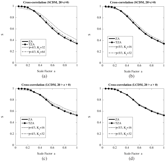
Figure 5: The same as Figure 4. In these figures, we changed the course-grained length to $l=2h^{-1}\mbox{Mpc}$.  (a) The SCDM model with $\gamma=4/3$.  (b) The SCDM model with $\gamma=5/3$.  (c) The LCDM model with $\gamma=4/3$.  (d) The LCDM model with $\gamma=5/3$.

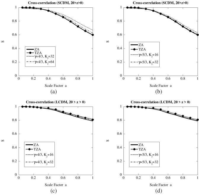
Figure 6: The same as Figure 4. In these figures, we changed the course-grained length to $l=4h^{-1}\mbox{Mpc}$.  (a) The SCDM model with $\gamma=4/3$.  (b) The SCDM model with $\gamma=5/3$.  (c) The LCDM model with $\gamma=4/3$.  (d) The LCDM model with $\gamma=5/3$.

When the model evolves to strongly nonlinear regime, the trend of the solutions change. In the linear stage, the case of $\gamma=4/3$ shows deviation from ZA. However in strongly nonlinear regime, though the Lagrangian approximation generally become worse, the case of $\gamma=4/3$ shows a rather good result (Figure 4 (a) and (c)). This tendency was unchanged even though the course-grained length was changed (Figure 5 and 6).

In both the SCDM and LCDM models, when we choose a small initial Jeans wavenumber $K_{J}$, although the approximation is improved after the quasi-nonlinear stage, the reasonable range of Jeans wavenumbers seems wide. The strict limitation to the value of $\kappa$ or the initial Jeans wavenumber will be given by other physical considerations or by the high-resolution N-body simulation.

From these results, we find that it is reasonable to choose the polytrope exponent $\gamma=5/3$ until quasi-nonlinear regime is reached. These results support the suggestion by Buchert and Domínguez budo and by Domínguez domi0103 . If we have interest in strongly nonlinear regime, although the Lagrangian approximation generally becomes worse, we had better analyze the case of $\gamma=4/3$. In this regime, it is necessary to consider whether that approximation will still be valid. In any case, from the cross-correlation coefficient, we can give limitation in the polytrope exponent $\gamma$.

Unfortunately, in these results, we cannot give a strict limit to the proportion coefficient $\kappa$ of the equation of state. When we choose $\gamma=4/3$, we show that the result strongly depends on $\kappa$, and we can notice a strict limitation. However when we choose $\gamma=5/3$, we can hardly judge the best value for $\kappa$. In our calculation, we found out that it was good to set up the initial ($a=10^{-3}$, i.e. $z=1000$) Jeans wavenumber $K_{J}$ as $N^{1/3}/4\leq K_{J}\leq N^{1/3}$. From the range of $K_{J}$, we can obtain a reasonable value for $\kappa$. If we choose large value for $\kappa$, it becomes hard to form nonlinear structure. On the other hand, if we choose small value for $\kappa$, the structure becomes almost the same as the structure which was obtained by ZA.

Although the cross-correlation coefficient is one thing which is good for checking the accuracy of the approximation, it is not enough for checking. Now we consider two samples A and B. The density contrast of the samples is given by $\delta_{A}$ and $\delta_{B}$, respectively. We assume that the following proportion relation exists between $\delta_{A}$ and $\delta_{B}$:

$$\delta_{A}\propto\delta_{B}\,.$$ (14)

Even if the density contrast is greatly different, as $\delta_{A}$ and $\delta_{B}$, and one shows a highly nonlinear structure and another remains in the linear regime, the cross-correlation coefficient between $\delta_{A}$ and $\delta_{B}$ becomes $1$.

Therefore, we must check the accuracy of the approximation with another property. In the next subsection, we analyze the probability distribution function of density fluctuation.

III.2 Probability Distribution Function of Density Fluctuation

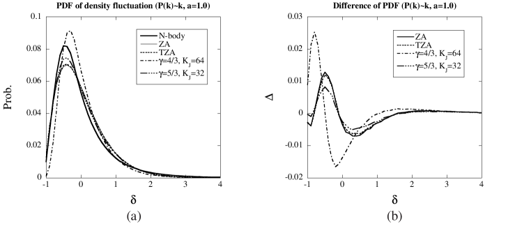
Figure 7: The PDF of density fluctuation for a scale-free spectrum ($P(k)\propto k$, $l=1h^{-1}\mbox{Mpc}$: $\sigma_{N-body}\simeq 1$ at $a=1.0$.).  (a) The PDF of density fluctuation. In the case of $\gamma=4/3$, the effect of pressure suppresses the growth of the fluctuation.  (b) The difference in the PDF of density fluctuation. In this figure, the difference between the case of $\gamma=4/3$ and other cases becomes clear. When we choose $K_{J}=32$ for the case of $\gamma=4/3$, more greater difference appears.

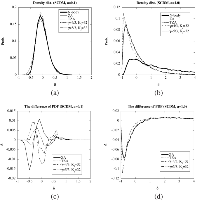
Figure 8: The PDF of density fluctuation in the SCDM model ($l=4h^{-1}\mbox{Mpc}$). In the case of $\gamma=4/3$, the pressure effect suppresses the growth of density fluctuation. Therefore the probability of a small fluctuation ($|\delta|<1$) increases.  (a) The SCDM model, at $a=0.1$ ($z=9$, $l=4h^{-1}\mbox{Mpc}$. Quasi-nonlinear regime). In the case of $\gamma=4/3$, the effect of pressure suppresses the growth of the fluctuation.  (b) The SCDM model, at $a=1.0$ ($z=0$, $l=4h^{-1}\mbox{Mpc}$. Strongly nonlinear regime).  (c) The difference in the PDF of density fluctuation between the N-body simulation and Lagrangian approximations. At $a=0.1$.  (d) Same as (c), but at $a=1.0$.

Here, we compare the probability distribution function (PDF) of density fluctuation. In the Eulerian linear approximation, if initial data is given by a random Gaussian distribution, the PDF of density fluctuations will retain its Gaussianity during evolution. On the other hand, in the Lagrangian approximation, there appears a nonlinear effect. In fact, Kofman et al. Kofman94 shows that the PDF of density fluctuation approaches a log-normal function rather than a Gaussian function in the cases of the Lagrangian approximation and N-body simulation. Padmanabhan and Subramanian PadSub93 also discussed the PDF of density fluctuation with the ZA and found a non-Gaussian distribution.

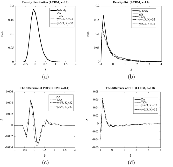
Figure 9: The PDF of density fluctuation in the LCDM model ($l=4h^{-1}\mbox{Mpc}$). In the case of $\gamma=4/3$, the pressure effect suppresses the growth of density fluctuation. Therefore the probability of a small fluctuation ($|\delta|<1$) increases.  (a) At $a=0.1$ ($z=9$, $l=4h^{-1}\mbox{Mpc}$. Quasi-nonlinear regime). The PDFs of density fluctuation seem similar to each other.  (b) At $a=1.0$ ($z=0$, $l=4h^{-1}\mbox{Mpc}$. Strongly nonlinear regime).  (c) The difference in the PDF of density fluctuation between the N-body simulation and Lagrangian approximations. At $a=0.1$.  (d) Same as (c), but at $a=1.0$.

How will the PDF of density fluctuation change if we take the effect of the velocity dispersion into consideration? Figures 7, 8, and 9 shows the PDF of density fluctuation. As in past works, the PDF of density fluctuation becomes log-normal in form in the N-body simulation. In Figures 7, 8, and 9, the cases of $\gamma=4/3$ obviously show the different tendency: in these cases, the effect of pressure suppress the growth of positive fluctuation (Figure 7(b), 8 (c),(d), and 9 (c),(d)). When we also consider the PDF of density fluctuation, we can notice that it is not so good to choose $\gamma=4/3$ to examine the growth of structure, though the cross-correlation coefficients well show the trend. On the other hand, the case of $\gamma=5/3$ well show the trend in the PDF of density fluctuation. Although the difference of distribution between ZA and the pressure model is still small in quasi-nonlinear regime, the effect of the pressure can promote the evolution of nonlinear structure. Therefore the probability of low and high density regions increases in the case of $\gamma=5/3$. Furthermore, according to Figure 8(c), the PDF of density fluctuation in the cases of $\gamma=5/3$ show that it is much better than that in the TZA case. Of course when we reach a strongly nonlinear regime, it is necessary to consider whether that approximation is still valid or not.

From both the cross-correlation coefficient and PDF of density fluctuation, we can decide that it is reasonable to choose $\gamma=5/3$ as the polytrope exponent of the equation of state. However it is hard to decide the proportional parameter $\kappa$. From the results in this paper, we cannot give tight limit to $\kappa$. To decide the value of $\kappa$, we will analyze a high-resolution N-body simulation or consider other physical processes. For example, we will consider the effect of anisotropic velocity dispersion mtm or the higher order velocity cumulant.

IV Discussion and Concluding Remarks

We compared two statistical quantities between an N-body simulation and Lagrangian approximations. In our earlier work moritate ; tate02 , we solved the first-order perturbation equations in the homogeneous and isotropic background, and the second- order ones explicitly for the case $\gamma=4/3,5/3$ in Einstein-de Sitter Universe. We showed that the difference between the Lagrangian first-order and second-order approximations becomes small in the case of $\gamma\geq 4/3$. Therefore, in this paper we consider only the first-order perturbative solution for the case $\gamma=4/3,5/3$. Then we carried out similar calculation with ZA and TZA to examine their difference from the past models.

First, we compared these models by the cross-correlation coefficient of the density field between the N-body simulation and Lagrangian approximations. In scale-free spectrum cases, as well as in the previous analyses, TZA shows a better performance than ZA. In the pressure model, the performance strongly depends on polytrope exponent $\gamma$ and Jeans wavenumber. In the case of $\gamma=4/3$, when we set that initial Jeans wavenumber to be small, even in linear regime the approximation deviates from the N-body simulation. In the case of $\gamma=5/3$, although the result slightly depends on the initial Jeans wavenumber, the pressure model shows a better performance than ZA in quasi-nonlinear regime. Furthermore, the pressure model also shows better performance than TZA. In the SCDM and LCDM models, the case of $\gamma=4/3$ shows deviation from ZA in linear regime. On the other hand, the case of $\gamma=5/3$ shows that the cross-correlation coefficient becomes almost the same in linear regime. When the model reaches a strongly nonlinear stage, although the Lagrangian approximation generally become worse, the case of $\gamma=4/3$ shows a rather good result. Of course, in this regime, it is necessary to consider whether that approximation is still valid.

Second, we analyzed the PDF of density fluctuation. The cases of $\gamma=4/3$ obviously show a different tendency until quasi-nonlinear regime is reached: in this case, the effect of pressure suppresses the growth of structure. When we also consider the probability distribution of density, we can see that it is not so good to choose $\gamma=4/3$ to examine the growth of structure, although the cross-correlation coefficients perform well. On the other hand, the case $\gamma=5/3$ shows good tendency in the PDF of density fluctuation. Although the difference of the PDF of density fluctuation between ZA and the pressure model is still small in quasi-nonlinear regime, the effect of the pressure can promote the evolution of nonlinear structure. The difference between the models of Lagrangian approximation becomes small when we calculate the evolution until strongly nonlinear regime is reached. From analyses of the cross-correlation coefficient of density field and the PDF of density fluctuation, we can decide that it is reasonable to choose $\gamma=5/3$ as the polytrope exponent of the equation of state.

In this paper, we changed some values of the Jeans wavenumber $K_{J}$ and undertook analysis. Will there be any relations between the ‘nonlinear wavenumber’ $k_{NL}$ in TZA and $K_{J}$ ? The correspondence is as follows. For simplification, we consider the correspondence in case of a scale-free spectrum $P(k)\propto k^{n}$. According to the definition of a ‘nonlinear wavenumber’ in TZA, $k_{NL}$ is given from Equation (10). In case of the scale-free spectrum $P(k)=Ak^{n}$, the definition becomes

$$\frac{1}{n+1}a(t)^{2}Ak_{NL}^{n+1}=1.$$ (15)

From this definition, $k_{NL}$ is written as

$$k_{NL}\sim a^{-2/(1+n)}.$$ (16)

For example, when we choose $n=1$, $k_{NL}$ becomes

$$k_{NL}\sim\frac{1}{a}.$$ (17)

On the other hand, the Jeans wavenumber $K_{J}$ in the pressure model is given from Equation (6). When we choose $\gamma=2$, $K_{J}$ becomes

$$K_{J}\sim\frac{1}{a}.$$ (18)

There are some different points to consider when we think about time evolution, although the relation seems to be as described above: First, in TZA, $k_{NL}$ affects only the initial spectrum. On the other hand, $K_{J}$ affects the evolution of fluctuation. Second, although $k_{NL}$ obviously depends on the initial spectrum, we did not clarify the dependence on the initial condition of $K_{J}$. We think that a consideration of the physical process, which was not considered here, or the analysis of the N-body simulation, is necessary for a decision of $K_{J}$, i.e. $\kappa$. We will have to think about the correspondence between the adhesion approximation and the pressure model. Buchert et al. bdp showed how the viscosity term in the adhesion approximation is generated by a pressure-like force. Domínguez domi00 ; domi0106 discussed spatial coarse graining in a gravitating system and derived an evolution equation of ‘adhesion approximation’. In the pressure model, we showed that the density distribution of the pressure model was similar to that of TZA in the previous paper tate02 . The acute characteristic skeleton structure which appeared in the adhesion approximation could not be seen from the calculations in our previous paper. We will consider the relation between the viscosity term in coarse-grained equations and the pressure term in our model. Then we will analyze the correspondence between the viscosity term in the adhesion approximation and the proportional constant $\kappa$ in equation of state in pressure model.

In this paper, we analyzed only density distribution. How will peculiar velocity distribution change with the effect of ’pressure’? In ZA, the peculiar velocity is in proportion to the Lagrangian displacement. Then the growth rate of perturbation is independent of scale. Therefore, although the structure becomes nonlinear regime, if the initial condition is given as Gaussian, the peculiar velocity distribution remains Gaussian all the time Kofman94 . However, in the pressure model, the growth rate of the perturbation depends on the scale. Therefore the peculiar velocity distribution will deviate from Gaussian during evolution. Of course, the peculiar velocity distribution in an N-body simulation becomes non-Gaussian ZQSW94 . Does the effect of the pressure cause the occurrence of the non-Gaussian distribution? We think that the time evolution of the peculiar velocity distribution is one of the more interesting problems.

In our model, we introduce the strong simplification that the velocity dispersion is approximately isotropic, i.e. the stress tensor is diagonal and a pressure-like term bdp . However, in general, the velocity dispersion does not remain isotropic in nonlinear regime. Until when is the assumption to ignore anisotropic velocity dispersion reasonable? Maartens et al. mtm discussed a relativistic kinetic theory generalization which also incorporates anisotropic velocity dispersion. Then they added these effects to the linear development of density inhomogeneity and found exact solutions for their evolution. In a Newtonian description, though the equations is not generally closed, we will consider anisotropic velocity dispersion and the higher-order velocity cumulant and estimate their effects on the evolution of density inhomogeneity.

- (1) Ya. B. Zel’dovich, Astron. Astrophys. 5, 84 (1970).
- (2) T. Buchert, Mon. Not. R. Astron. Soc. 254, 729 (1992).
- (3) P. Coles and F. Lucchin, Cosmology: The Origin and Evolution of Cosmic Structure (John Wiley & Sons, Chichester, 1995).
- (4) V. Sahni and P. Coles, Phys. Rep. 262, 1 (1995).
- (5) D. Munshi, V. Sahni, and A. A. Starobinsky, Astrophys. J. 436, 517 (1994).
- (6) V. Sahni and S. F. Shandarin, Mon. Not. R. Astron. Soc. 282, 641 (1996).
- (7) M. Davis, G. Efstathiou, C. S. Frenk, and S. D. M. White, Astrophys. J. 292, 371 (1985).
- (8) Ya. B. Zel’dovich, Sov. Astron. 26, 289 (1982).
- (9) É. V. Kotok and S. F. Shandarin, Sov. Astron. 31, 600 (1987).
- (10) S. F. Shandarin and Ya. B. Zel’dovich, Rev. Mod. Phys. 61, 185 (1989).
- (11) S. N. Gurbatov, A. I. Saichev, and S. F. Shandarin, Mon. Not. R. Astron. Soc. 236, 385 (1989).
- (12) P. Coles, A. L. Melott, and S. F. Shandarin, Mon. Not. R. Astron. Soc. 260, 765 (1993).
- (13) A. L. Melott, T. F. Pellman, and S. F. Shandarin, Mon. Not. R. Astron. Soc. 269, 626 (1994).
- (14) J. Binney and S. Tremaine, Galactic Dynamics (Princeton University Press, Princeton, NJ, 1987).
- (15) T. Buchert and A. Domínguez, Astron. Astrophys. 335, 395 (1998).
- (16) T. Buchert, A. Domínguez, and J. Perez-Mercader, Astron. Astrophys. 349, 343 (1999).
- (17) A. Domínguez, Phys. Rev. D 62, 103501 (2000).
- (18) A. Domínguez, Mon. Not. R. Astron. Soc. 334, 435 (2002).
- (19) A. Domínguez, Astron. Nachrichten 324, 560 (2003).
- (20) A. Domínguez and A. L. Melott, astro-ph/0310693.
- (21) S. Adler and T. Buchert, Astron. Astrophys. 343, 317 (1999).
- (22) M. Morita and T. Tatekawa, Mon. Not. R. Astron. Soc. 328, 815 (2001).
- (23) T. Tatekawa, M. Suda, K.I. Maeda, M. Morita, and H. Anzai, Phys. Rev. D 66, 064014 (2002).
- (24) E. Bertschinger, Astrophys. J. Supp. 137, 1 (2001).
- (25) A. L. Melott, S. F. Shandarin and D. H. Weinberg, Astrophys. J. 428, 28 (1994).
- (26) T. Buchert, A. L. Melott, and A. G. Weiss, Astron. Astrophys. 288, 349 (1994).
- (27) A. L. Melott, T. Buchert, and A. G. Weiss, Astron. Astrophys. 294, 345 (1995).
- (28) G. Karakatsanis, T. Buchert, and A. L. Melott, Astron. Astrophys. 326, 873 (1997).
- (29) L. Kofman, E. Bertschinger, J. M. Gelb, A. Nusser, and A. Dekel, Astrophys. J. 420, 44 (1994).
- (30) T. Padmanabhan and K. Subramanian, Astrophys. J. 410, 482 (1993).
- (31) W. H. Zurek, P. J. Quinn, J. K. Salmon, and M. S. Warren, Astrophys. J. 431, 559 (1994).
- (32) R. Maartens, J. Triginer, and D. R. Matravers, Phys. Rev. D60, 103503 (1999).