The Effect of Clouds on Air Showers Observation from Space

Abstract

Issues relating to extensive air showers observation by a space-borne fluorescence detector and the effects of clouds on the observations are investigated using Monte Carlo simulation. The simulations assume the presence of clouds with varying altitudes and optical depths. Simulated events are reconstructed assuming a cloud-free atmosphere. While it is anticipated that auxiliary instruments, such as LIDAR (LIght Detection And Ranging), will be employed to measure the atmospheric conditions during actual observation, it is still possible that these instruments may fail to recognize the presence of a cloud in a particular shower observation. The purpose of this study is to investigate the effects on the reconstructed shower parameters in such cases. Reconstruction results are shown for both monocular and stereo detectors and for the two limiting cases of optically thin, and optically thick clouds.

${}^{\textrm{1}}$University of Utah, Department of Physics and High Energy Astrophysics Institute, Salt Lake City, Utah, USA

1 Introduction

Space-borne cosmic rays detectors for energies E $\geq 10^{20}$ eV have been proposed [1] and are now under study [2]. Such a detector will comprise one or two satellites orbiting the Earth at an altitude of $\sim$ 400 km to $\sim$ 1000 km and will have a wide field of view (FOV), on the order of 60^o. The footprint on the Earth’s surface of the FOV has dimensions on the same order of magnitude as the orbit height. Studies of the global distribution of clouds and their frequency of occurrence, e.g. [3], suggest that the target volume will at any point in time contain some clouds.

The amount of clouds (fractional cover), the distribution of clouds in terms of cloud type, altitude, and optical depth will undoubtedly affect the detector’s trigger aperture. In addition, cloud presence could result in a reduction of the reconstructible aperture, as contaminated events are excluded from the analysis. Finally cloud presence could compromise the accuracy of the energy estimate for an observed event, since this estimate depends in part on a knowledge of the atmospheric conditions at the time and location of the shower development and along the path the light from the shower travels to the detector.

The effect of cloud presence on the detector aperture is beyond the scope of this paper. In this study we limit our attention to the question of how cloud presence may affect the reconstructed shower geometry and energy. In the context of a Monte Carlo study, this question can be addressed by applying the event analysis assuming no cloud presence, and then determine (a) whether the reconstruction procedure can identify the presence of otherwise unreported clouds, and thereby rejecting the event in question, and (b) for those events where clouds eluded all detection attempts, how the reconstructed shower parameters were altered.

With respect to the detector itself, there are two possible modes of operation: monocular and stereo, the latter employing two sites (satellites) separated by some distance and which view the same region of the sky. The Fly’s Eye experiment has demonstrated the superiority of the stereo technique on the ground [4]. For space-borne detectors, it has been suggested [5] that monocular observation can perform as well as stereo if use is made of the information provided by the reflection of the Čerenkov beam associated with the shower off the surface of the Earth, in order to reconstruct the shower geometry. In this study we also investigate possible errors introduced in cases where the reflection occurs off the top of a cloud instead of the surface.

The answer to (a) above will depend on whether or not cloud presence will manifest itself through a significant alteration in the expected detector response to the shower signal. As an example, the reflectivity of an optically opaque cloud is several times larger than that of the surface of the ocean, $\sim 80$%-90% vs. $\sim 10$%-20%, therefore a test may be be developed and applied to an individual shower observation looking at the signal strength of the last few pixels to determine whether the reflection of the beam has occurred off the top of a cloud. The development of such a test is not trivial. It must be applicable to a wide range of shower energies and geometries as well as accommodate different atmospheric conditions and cloud optical properties. Also, the formulation of such a test must rely on a detailed description of the event data recorded by the detector for each shower observation. As described in section 3.1, we do not attempt a detailed simulation of the detector data acquisition system and event formation logic. Also, we only treat a few combinations of shower geometries and clouds configurations. Therefore, the development of a test for cloud presence based on the event data is beyond the scope of this study.

Clouds come in a wide variety of cloud types, heights, vertical extent, and optical depths. There are, in general, also spatially in-homogeneous and finite, a few kilometers in lateral extent, clouds. This makes a general treatment of all possible scenarios difficult. To simplify the discussion we will concentrate on two limiting cases. The first case is that of a high altitude, optically thin cloud. This case corresponds to cirrus clouds which are pervasive in the atmosphere [3]. The second case is that of low altitude, optically thick clouds. These types of clouds are easy to detect in general but may be difficult to detect under some circumstances, e.g., if the cloud is small in lateral size (on the order of a few kilometers.)

This paper is organized as follows: The next section provides a motivation for the different cloud configurations used in the study. Following that is an overview of the Monte Carlo simulation of the detector, showers, and the atmosphere including cloud simulation. Section 4 provides an overview of the shower geometry and energy reconstruction procedures. Finally section 5 presents the results of the study.

2 Clouds and EAS

Clouds are classified as (a) low-level (cloud base height, $h_{base}<2$ km), (b) mid-level ($2<h_{base}<6$ km), and (c) high-level( $h_{base}>6$ km) [6]. In the equatorial region, high-level clouds (Cirrus) typically occur at altitudes of $8-15$ km [6]. Most EAS develop in the lower atmosphere at altitudes < 20 km, where most of the atmospheric mass is located. Depending on their altitude, clouds are made up of predominantly water molecules, (low-level), mixed water molecules and ice crystals (mid-level), and ice crystals (high-level). For our purposes, water and ice crystal clouds have one important difference: the number density of scatterers. The concentration of water molecules in a low level cloud is a factor of 10 to 100 greater than that of ice crystals in a high altitude cirrus cloud. This results in a much smaller scattering length for the low level cloud, and the relation between the optical depth of the cloud and its physical thickness becomes qualitatively different.

From detailed Monte Carlo simulations, most EAS generated by protons or nuclei in the energy range $10^{19}\leq E\leq 10^{21}$ eV reach maximum development at atmospheric slant-depths, $x$, between 700-1000 gm/cm² (depending on the energy, primary type, and the hadronic model used in the simulations) [7]. Beyond the shower maximum depth, $x_{max}$, the number of electrons in the shower falls rapidly.

To quantify how clouds might affect space-borne observations of extensive air showers, we need to relate the atmospheric slant depth along the shower track to altitude above the Earth’s surface (sea level). This relation depends on the shower zenith angle and is presented in figure 1 and table 2. As can be seen from the table, different cloud altitude and shower zenith angle combinations can result in the shower front reaching the cloud top at different stages of the shower development. Three broad cases can be identified: (1) clouds above shower development, (2) clouds in the region of shower development, and (3) clouds below shower development.

Table 1: The height (km) above the surface, of a point along the shower track at a given slant depth (gm/cm${}^{2})$ along the shower, for showers with different zenith angles, $\theta$. Atmospheric density profile according to the U.S. Standard Atmosphere, 1976.

$x_{slant}$ \ $\theta$	30	45	60	75	85
200	12.81	14.08	16.23	20.13	24.84
400	8.31	9.67	11.85	15.79	20.65
600	5.43	6.89	9.25	13.25	18.24
800	3.24	4.79	7.28	11.45	16.53
1000	1.46	3.07	5.68	10.04	15.21
1200	-	1.62	4.32	8.85	14.13
1400	-	0.34	3.14	7.80	13.22
1600	-	-	2.07	6.88	12.43

Figure 1: Slant depth (g/cm²) along a shower track with a zenith angle, $\theta$, vs. the height (km) above the surface of a point along the shower track. Data from table 1.

In addition to the location of the cloud in relation to the shower-detector geometry, the optical depth, $\tau$, and physical thickness, $\Delta z$, of the cloud also play a role in determining what the detector sees. Hence they also need to be considered in combination with the height of the cloud top, $h_{top}$. Finally, depending on the values of $\tau$ and $\Delta z$, the effects of multiple light scattering may or may not be negligible, $\lesssim$10%.

As mentioned in the introduction, we will only address the two limiting cases for the optical depth. The reason for this is that the consideration of these cases is sufficient for the study of the relevant problems of: light transmission through high altitude cirrus clouds (optically thin), and the Čerenkov beam reflection off optically thick clouds and its effect on the monocular geometry reconstruction. In general, single scattering calculations are sufficient for a medium $\tau<0.1$. First order corrections may be required for $0.1<\tau<0.3$ [8, 9]. From our own studies, we saw that for $\tau<0.5$, second order corrections account for less than $\sim$ 10% of the total signal transmitted through a cloud. Therefore, to avoid having to calculate light multiple scattering beyond first order corrections we will restrict our definition of optically-thin clouds to mean clouds with optical depth $\tau<0.5$.

For the case of an opaque cloud, a light beam impinging on the top of the cloud will be reflected as a result of a large number of multiple scatterings inside the cloud. The amount, spatial and temporal distributions, and the direction of the reflected photons can be calculated using a Monte Carlo procedure (see section A.3). The use of this procedure or an equivalent detailed simulation of the cloud reflective properties would be required if one is to attempt to infer the cloud presence from the event data. For this study, however, it is sufficient to treat reflection off clouds in the same fashion as reflection off the surface, as described in section 3.4.

3 Simulation

Both the simulation and reconstruction programs used in this study are based on those developed for the High Resolution Fly’s Eye (HiRes) experiment [10]. The original programs are described in detail in [11]. While the underlying algorithms are similar to those used by HiRes, the actual code was converted from Fortran and C to the C++ language and extensive use was made of the ROOT data analysis framework [12].

Naturally, the HiRes detector simulation was replaced by a description of the OWL detector. Otherwise, a large portion of the simulation code, e.g. the atmosphere, is detector independent, and was retained. Cloud simulation including the effects of multiple light scattering was added, and minor modifications were made throughout the code to account for the differences between the two detectors.

In the following subsections a description of the detector simulation is given, followed by a synopsis of the atmospheric modeling. We then present an overview of the shower simulation, and the section ends with a discussion of the Čerenkov spot.

3.1 The Detector

A description of the OWL baseline instrument is given in [13]. Earlier versions of proposed designs were presented in a workshop [2]. Our detector simulation is based on these earlier designs. The conclusions drawn from these studies will not be substantially affected by the design evolution. A description of the simulated detector follows:

The detector consists of two cameras, each mounted on a satellite. The satellites have an orbital height of 800 km and are separated by a distance of 500 km. Each camera comprises a concave, spherical mirror and a focal plane detector. The mirror has an effective light collecting area of 4.9 m² and a field of view (FOV) corresponding to a cone of half-angle of 30^o. The mirrors axes are tilted slightly from the nadir in order for the two cameras to view a common area on the surface.

For the reason that the optical design of the detector had not been completed at the time this study was begun, and also for the sake of simplicity, we opted to use a scheme in which all photon ray-tracing calculations are done in angular space. In this case we ignore the details of the detector optics and simply treat the mirror as a “light collector” with a circular aperture. The focal plane pixels are arranged on a rectangular grid with each pixel having a fixed angular size. The pixel angular size is selected to meet the detector design requirement of resolving a distance of 1 km on the surface. So, for an orbit height $h$, the pixel angular size, $\delta$, is equal to $1/h$ radian, with $h$ measured in km’s. For a 800 km orbit this translates to $\delta\approx 0.7^{o}$. We assume full coverage of the focal surface, i.e., we ignore the physical gaps and dead areas between the PMT’s.

During an event simulation we calculate and record the arrival time of each photon reaching the detector from the shower. The arrival direction of the photon determines the pixel in which the photon is registered. Data for a triggered pixel comprises the pixel pointing direction, the integrated pixel signal and the mean arrival time of the photons recorded by the pixel. The integrated signal is simply the number of photo-electrons (pe) recorded by the pixel in a time window of 12 $\mu$s. The particular choice for the width of the time window allows enough time for a shower with a zenith angle of 30^o or greater to cross the field of view of the pixel.

We employ a simple detector trigger scheme, which requires at least six pixels to fire from the light of the shower in order to form an event. A pixel trigger occurs if the pixel records three or more pe in a one $\mu$s interval. The test for an individual pixel trigger is performed as follows:

1. the arrival times for each of the pe recorded by the pixel are sorted in time to find the arrival times of the first and last recorded pe A time window is formed around these times, and a 2 $\mu s$ interval is added to each end.

2. sky noise pe are added to the expanded time window assuming a uniform background of 200 photons/m²/sr/ns.

3. shower generated and noise pe are now stored in a histogram with a 1 $\mu$s bin width. The histogram’s bins are scanned and if any bin has three or more entries then the pixel trigger flag is set.

4. finally, if the total width of the time window exceeds 12 $\mu$s, then a sliding window of that width is used to scan the histogram to find the set of contiguous bins with the largest sum.

Finally, we incorporate elements from the HiRes detector to cover some of the gaps in the simulation. In particular we assume that the detector will use a UV filter similar to that of HiRes, which passes light in the 300-400 nm range. A parameterization of the wavelength dependence of the PMT quantum efficiency is also borrowed from the HiRes simulation, so is a constant mirror reflectivity of 80%. These detector components are described in detail in [10].

3.2 The Atmosphere

There are four elements or components to the simulation of UV light transmission through the atmosphere. These include Rayleigh scattering by molecules of air, scattering by surface aerosols, absorption by ozone molecules, and scattering by clouds. The treatment of the first three is based on the HiRes simulations; we adopted the same models without modifications. Although these models are more appropriate for the Utah desert observation conditions than for observation over the ocean, the differences should have little effect on the results of this study. This is because the shower development and light propagation to the satellites occur almost entirely above the surface aerosol layer, which is the one factor most likely to be significantly different between the desert and the ocean. Before we turn to a discussion of the cloud simulation we present a brief overview of these models.

Light scattering is characterized by the scattering cross section, $\beta$, and the phase function, $P=P(\cos\theta_{s})$, where $\theta_{s}$ is the scattering angle. The cross section for molecular, or Rayleigh, scattering is given by:

$$\beta_{R}=100(\rho(h)/x_{R})(400/\lambda)^{4}$$ (1)

where $\beta_{R}$ is measured in units of $m^{-1}$, $\rho(h)$ is the air density (g/cm²) at altitude $h$ (m) above sea level, and $x_{R}=2970$ g/cm² is the mean free path at wavelength $\lambda=400$ nm. The air density and temperature profiles as function of altitude are given by the U.S. Standard Atmosphere, 1976 [14]. The phase function for Rayleigh scattering is given by:

$$P(\cos\theta_{s})=(3/16\pi)\left(1+\cos^{2}\theta_{s}\right)$$ (2)

Aerosols scattering is calculated according to the following formula:

$$\frac{dN}{dl}=-\frac{N}{L_{a}(\lambda)}\rho_{a}(h)$$ (3)

Here $L_{a}$ is the scattering length at the surface, and we have:

$$\beta_{a}(\lambda)=\rho_{a}/L_{a}(\lambda)$$ (4)

The aerosols reduced density, $\rho_{a}$, is given by:

$$\rho_{a}=\left\{\begin{array}[]{cc}1&h<h_{m}\\ e^{-(h-h_{m})/H_{a}}&h\geq h_{m}\end{array}\right.$$ (5)

where $h_{m}$ is the height of the mixing layer, and $H_{a}$ is the scale height above the mixing layer [15]. The scattering length at wavelength $\lambda=334$ nm is a free parameter of the model. The wavelength dependence of the scattering process is accounted for by a parameterization, shown in figure 2. The aerosols scattering phase function, also shown in figure 2, is based on the Longtin desert aerosols model [16]. For this study, the model parameters are set to: $h_{m}=0$, $H_{a}=1.2$ km, and $L_{a}(334)=23.0$ km.

Ozone absorption is characterized by a wavelength-dependent absorption coefficient, $\alpha_{O3}$, and an altitude-dependent concentration, $\rho_{O3}$, both shown in figure 2. Model parameters were extracted from [17]. The extinction length, in meters, due to ozone absorption can be written as:

$$\frac{1}{L_{O3}}=(9.87\times 10^{-7})\times\alpha_{O3}(\lambda)\times\rho_{O3}(h)$$ (6)

with the constant factor accounting for unit conversion.

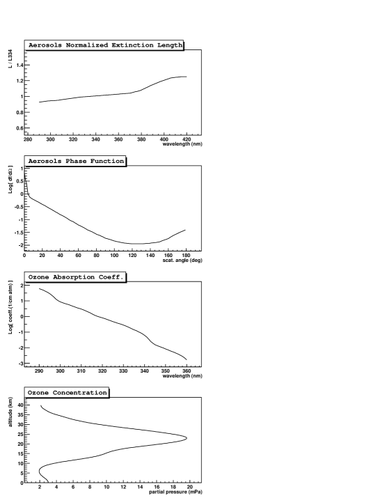
Figure 2: From the top, the wavelength dependence of the aerosols extinction length, the aerosols phase function, the wavelength dependence of ozone absorption, and the ozone concentration as a function of altitude.

The cloud model and the simulation of light propagation in a cloud is described in detail in appendix A. Here we present a brief description of the model.

Simulated clouds have a uniform density which steps to zero at the cloud boundaries. The parameters used to describe a cloud are the cloud base height, $h_{base},$ cloud top height, $h_{top}$, and the optical depth $\tau$. The scattering length, $\beta$, inside the cloud is related to the optical depth by the relation:

$$\tau=\beta(h_{top}-h_{base})$$ (7)

The wavelength dependence of the scattering process, which is mild in the near UV [18], is ignored. Finally, scattering within optically thin clouds calculatioins use a phase function appropriate for ice clouds at $\lambda=0.5$ $\mu$m [19].

3.3 Shower Simulation

The primary particle energy is selected at the start of the simulation. The shower track geometry is generated randomly in order to obtain uniform and isotropic showers distributions in the atmospheric volume viewed by the detector.

The generated shower profiles follow a Gaisser-Hillas function [20]. The number of electrons, $N_{e}$, in the shower is given as a function of depth, $x$, by:

$$N_{e}(x)=N_{max}\left(\frac{x-x_{0}}{x_{max}-x_{0}}\right)^{(x_{max}-x_{0})/\lambda}e^{(x_{max}-x)/\lambda}$$ (8)

where the $x_{0}$ parameter is chosen from an exponential ($<x_{0}>=$35 g/cm² for proton primaries), $x_{max}$ is chosen from a Gaussian distribution, $\lambda$ is fixed at 70 gm/cm², and $N_{max}$ is selected so that the integral of the profile, corrected for lost energy [21] [22], gives a total shower energy equal to that of the primary particle:

$$E_{tot}=E_{corr}+2.18\times\int N_{e}dx$$ (9)

The mean and variance of the $x_{max}$ Gaussian distribution depend on the energy and mass number of the primary cosmic ray particle. For protons we assume $<x_{max}>=725$ g/cm² at $E=10^{18}$ eV, increasing by 55 g/cm² per decade in energy. The standard deviation is set to 50 g/cm² for all energies. These values are based on shower simulations quoted by the Fly’s Eye group in their analysis [23], and are consistent with simulations results from the corsika program with the QGSJet model [7].

The Nishimura-Kamata-Greisen (NKG) function [24, 25], is used to describe the lateral distribution of shower electrons:

$$\rho_{e}(r)=\frac{N}{r^{2}}f\left(s,\frac{r}{r_{M}}\right)$$

where

$$f=\frac{\Gamma(4.5-s)}{2\pi\Gamma(s)\Gamma(4.5-2s)}\left(\frac{r}{r_{M}}\right)^{s-2}\left(1+\frac{r}{r_{M}}\right)^{s-4.5}$$ (10)

and the shower age parameter, $s$, is given by:

$$s=3x/(x+2x_{max})$$ (11)

Here, $r_{M}$ is the Molière radius. The value of $r_{M}$ depends on the air density and is evaluated at each point along the track.

Fluorescence light is generated according to the formulas given in [15], but more recent measurements of the air fluorescence yield are used [26]. The calculation of the Čerenkov light production also follows that of the Fly’s Eye paper [15].

The above procedure is modified if optically thin clouds are present. First we identify all track segments which lie inside the cloud. For these segments the simulation proceeds as described above but in addition, the number of fluorescence photons scattering once in the cloud, and Čerenkov photons scattering once or twice in the cloud, before reaching the detector, are calculated. These photons are included in the detector response as additional signal.

3.4 Čerenkov Spot

The Čerenkov spot refers to the area on the surface around the shower core where the Čerenkov beam is reflected, off the surface and into the detector. The simulation of the signal recorded by the detector, and generated by the reflected beam, requires the consideration of three separate issues: (1) The lateral distribution of the Čerenkov photons at a given point along the shower development, (2) the lateral distribution of the Čerenkov photons at the surface, and (3) the reflection properties of the surface.

The lateral distribution of photons in the Čerenkov beam is assumed to follow that of the shower electrons, i.e. it’s given by the NKG function. This is a simplification and in general results in a greater concentration of Čerenkov photons near the shower axis. A more accurate description of the lateral spread of the Čerenkov beam would be required ( along with a detailed detector simulation ) to address the problem of identifying cloud presence from event data. For this study, however, the use of the NKG function is sufficient.

The Čerenkov front has a circular shape centered around, and perpendicular to the shower axis. The spot formed on the surface by the beam is in general elliptical with the elongation of the spot depending on the zenith angle of the shower. In the simulation, the transformation of the photon position from a point on a circular disk about the shower axis to a point on the reflecting surface is performed and the time offset of the photons relative to the shower core is calculated before the photon is propagated to the detector.

Finally, the surface reflection albedo is assumed to be constant at 20% for reflection off water, and the reflection is assumed to be isotropic (into $2\pi$). The same is assumed for cloud reflection.

4 Event Reconstruction

Events are reconstructed from the raw event data to obtain the shower energy, shower $x_{max}$ , and the arrival direction of the primary cosmic ray particle. The raw data consists of a set of triggered pixels with known pointing directions, each with a measured mean arrival time and a time-integrated total pe count. With two instruments observing the shower, the combined data from each instrument comprises a stereo event. Data from each instrument can be analyzed separately as a monocular event.

The reconstructed shower is described by a set of parameters which specify the shower geometry and shower profile. The shower energy is obtained from the shower profile using eq. 9. The shower track geometry can be described by a pair of orthogonal vectors $\vec{R}_{p}$ and $\hat{u}_{t}$, the latter being the shower direction unit vector. Alternatively the geometry can be specified in terms of the Shower-Detector (SD) plane normal, $\hat{n}$, and a pair of scalars $R_{p}$ and $\psi$ which determine a line in that plane. The shower profile is given by the Gaisser-Hillas function, eq. 8.

Event reconstruction is divided into three consecutive steps:

1. SD plane reconstruction for each eye.

2. Shower track geometry reconstruction.

3. Shower profile and energy reconstruction.

Step 2. above is implemented differently for monocular and stereo events. For stereo, the intersection of the two SD planes from each eye determines the shower track. Monocular reconstruction requires the use of pixel trigger timing and an additional constraint provided by the observation of the Čerenkov spot. All other steps are similar for both monocular and stereo events.

In general, a file containing a set of Monte Carlo generated events contains a reference to the set of atmospheric parameters used in the simulation. This enables the reconstruction programs to use the same atmosphere used in the simulation. However, since the purpose of this study is to investigate the effect of clouds which go undetected, on the event reconstruction, clouds are removed from the atmosphere during reconstruction.

4.1 Shower Geometry

4.1.1 Shower-Detector Plane

The shower-detector plane is that plane which contains the detector, a point, and the shower track, a line. For a stereo detector a SD plane is calculated separately for each eye. The SD plane is calculated by minimizing a $\chi^{2}$ function given by:

$$\chi^{2}=\sum_{i}\frac{[(\hat{n}\cdot\hat{n}_{i})]^{2}\cdot w_{i}}{\sigma_{i}^{2}}$$ (12)

where the sum is over triggered pixels, $\hat{n}$ is the plane normal, $\hat{n}_{i}$ are the pixel viewing direction vectors and $w_{i}$ are weights equal to the total number of pe seen by pixel $i$. An angular pointing error of $\sigma\sim 0.07^{o}$ (equal to the pixel angular size) is assumed for all pixels.

4.1.2 Shower Track in the SD plane

In the case of stereo observation, the intersection of the SD plane normals from each eye describes a line in space, namely the shower track. This method despite its simplicity works very well in general [27]. Only events for which the opening angle between the two planes is small and the plane determination was not good, e.g. due to short track-length, does the method fail to produce accurate results.

In the case of monocular observation, track reconstruction uses the pixel timing information. The timing fit method is based on the relation between the crossing time of the shower front in a pixel’s field of view (mean photon arrival time at the detector) and the pixel’s viewing angle. The pixel crossing time $t_{i}$ as a function of the pixel viewing angle $\chi_{i}$ in the SD plane, is given by:

$$t_{i}=t_{0}+\frac{R_{p}}{c}tan\frac{1}{2}(\pi-\psi-\chi_{i})$$ (13)

The reader can refer to [15] for a derivation and definition of the parameters. In all, there are three unknown fit parameters, namely $t_{o}$ , $R_{p}$, and $\psi$.

A fit based on eq. 13 produces accurate results only when the range of angles covered by the triggered pixels, i.e. the angular track-length of the event, is “large enough”. A good discussion of the timing relation and the requirements for accurate reconstruction appear in [28] in relation to the Auger detector. For showers observed from space, the angular track-length is too small for the fit to result in satisfactory results, and an additional constraint on the shower geometry is required. The observation of the Čerenkov spot provides this constraint in the form of a known shower impact point on the surface, also referred to as the shower core position. The use of this constraint results in a significant improvement in the accuracy of the fit. The shower core vector is obtained from the event data as follows:

If the reflected Čerenkov light is observed by one pixel with a pointing direction vector $\hat{v}_{c}$ then, the shower core vector can be calculated using the relation $\vec{r}_{c}=\vec{r}_{m}+s\hat{v}_{c}$ where $\vec{r}_{c}$ is the shower core position, $\vec{r}_{m}$ is the detector position vector, and $s$ is a scalar which can be solved for by making the requirement that this line intersect the surface of the Earth (a sphere with a known radius corresponding to an altitude of $h=0$ m above sea level).

In general, the reflected light is observed by one or more pixels, to identify which we examine the set of triggered pixels for the one that triggered last in time and the one triggered last in angular distance from the start of the track. A group of one or more pixels is first identified as being triggered by the reflected beam by examining those pixels adjacent to the last triggered pixel for their trigger times. A sum of the pointing directions of these pixels (weighted by the total signal in each pixel) is performed to get an average direction. This direction is then projected in the SD plane to get a final estimate of the core direction.

4.2 Shower Profile

With the shower track geometry in hand we proceed to reconstruct the shower profile. The shower profile is assumed to follow a Gaisser-Hillas function with three free parameters: $x_{0}$, $x_{max}$, and $N_{max}$. For each trial profile a shower is generated with the reconstructed geometry and the detector response to the shower is calculated. The calculation proceeds along the same lines as the Monte Carlo (same light production and propagation models) with the exception that all random fluctuations are suppressed. Where in the MC the number and starting position of ray-traced photons is chosen randomly; During reconstruction, the mean number of photons from each track segment is distributed on a two dimensional grid representing an NKG lateral distribution. The effect of the finite mirror spot size is accounted for by distributing the flux received by the detector among the pixels according to the distribution of the spot.

The best fit (reconstructed shower profile parameters) is chosen to minimize a $\chi^{2}$ function calculated from the observed (MC output) and fit values for the pe counts from each pixel in the event. The following function is used:

$$\chi_{pfl}^{2}=\sum_{i}\frac{1}{\sigma_{i}^{2}}(S_{i}^{(m)}-S_{i}^{(p)})^{2}$$ (14)

where the sum is over triggered pixels, $S_{i}^{(m)}$ is the measured pixel signal in pe, $S_{i}^{(p)}$ is the predicted pixel signal, and $\sigma_{i}^{2}=S_{i}^{(m)}+B_{i}$. The $\sigma_{i}^{2}$ terms are obtained by adding in quadrature the Poisson fluctuation in the signal, $\sqrt{S^{(m)}}$, and the estimated sky background fluctuations for that pixel. It should be noted that not all triggered pixels are included in the sum. Those pixels near the end of the track believed to be triggered by the reflected Čerenkov beam are excluded from the sum.

5 Results and Conclusions

In this section we summarize the results obtained from the two studies of the possible effects of cloud presence on the reconstructed shower energies and $x_{max}$. We start with optically thin clouds.

5.1 Optically Thin Clouds

The effect of cloud presence is examined as follows: A Monte Carlo shower is generated in a cloud free atmosphere and the detector response is evaluated. Next, a loop over a set of cloud configurations (described below) is made in which the selected cloud is included in the atmosphere simulation. The same shower from the cloud free simulation is developed through the atmosphere, and the detector response is recorded. All events are reconstructed assuming a cloud free atmosphere.

Of the many (infinite) possible cloud configurations we selected the following set: Cloud base height is set to 6 km for all clouds in the study. Four different cloud top heights are used, these are given in table 2 along with the corresponding atmospheric slant depths along shower tracks at 60^o and 75^o. At each cloud top height setting, the cloud optical depth is varied between 0.1-0.5 in steps of 0.1, for a total of 20 cloud settings. Most Proton initiated showers with an energy of $10^{21}$ eV are expected to have $x_{max}$values in the range of 800-1000 g/cm². If these showers develop at a zenith angle of $60^{o}$ then they will reach maximum development at an altitude just above the selected cloud base height. In most cases then the shower will traverse the cloud while it is still increasing in size. At $\theta=75^{o}$, A cloud top height of 7.28 km or 9.25 km insures that the cloud lies below the shower $x_{max}$. The other cases cover a larger portion of the shower development curve.

Table 2: slant depth (gm/cm²) vs. height (km) for showers with zenith angles of $60^{o}$and 75^o. The values shown in the first column are chosen

$h$ (km) \ $\theta$	60o	75o
6.00	956	1810
7.28	800	1512
9.25	600	1130
11.85	400	751
16.23	200	372

Figures 3 through 6 summarize the results for stereo and monocular reconstruction of shower energy and $x_{max}$. In the figures, the cloud optical depth, $\tau$, is plotted along the $x$-axis, with $\tau=0$ corresponding to the cloud free atmosphere. Four points for each $\tau>0$ correspond to the different $h_{top}$ values. Cloud $h_{top}$ values of 7.28 km and 16.23 km are explicitly indicated on the plots by their corresponding slant depth values at $\theta=60^{o}$. Each point in the plots represents the mean shift and standard deviation for a set of 200 reconstructed events.

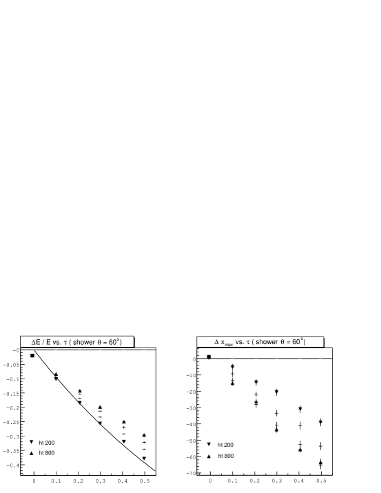
Figure 3: Energy and $x_{max}$ shift in the presence of optically thin clouds ( $\tau$ plotted along the $x$-axis ) for four different cloud top height settings, indicated by “ht 200” through “ht 800” . Stereo reconstruction of showers with $\theta=60^{o}$. The function, $\exp(-\tau)-1$, is superimposed on the energy plot.

Figure 4: Energy and $x_{max}$ shift in the presence of optically thin clouds ( $\tau$ plotted along the $x$-axis ) for four different cloud top height settings, indicated by “ht 200" through “ht 800". Stereo reconstruction of showers with $\theta=75^{o}$.

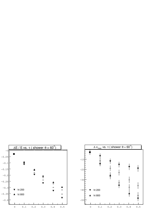
Figure 5: Energy and $x_{max}$ shift in the presence of optically thin clouds ( $\tau$ plotted along the $x$-axis ) for four different cloud top height settings, indicated by “ht 200" through “ht 800". Monocular reconstruction of showers with $\theta=60^{o}$.

Figure 6: Energy and $x_{max}$ shift in the presence of optically thin clouds ( $\tau$ plotted along the $x$-axis ) for four different cloud top height settings, indicated by “ht 200" through “ht 800". Monocular reconstruction of showers with $\theta=75^{o}$.

In the case of stereo reconstruction, the reconstructed shower geometry is unaffected by cloud presence. The cloud affects the amount of light reaching the detector from different parts of the shower depending on its position and extent. In a couple of cases the effect can be easily understood. For example, the case of $h_{top}=16.23$ km (ht 200 in the plot) and shower $\theta=60^{o}$, the mean reconstructed energy is shifted down by a factor of $\exp(-\tau)$. Another example is provided by the $\theta=75^{o}$ showers when the cloud lies well below shower maximum ($h_{top}$= 7.28 km or 9.25 km), in these cases we see very little effect on the reconstructed shower parameters.

The dependence of monocular shower geometry reconstruction on the observation and correct identification of the Čerenkov spot makes the interpretation of the results more complicated. In general, if the shower geometry is reconstructed correctly, then the effect of the cloud on the reconstructed energy and $x_{max}$ will be similar to the effect on stereo reconstructed events. Otherwise, the error will depend mostly on what the reconstructed geometry turns out to be. Looking at the $\theta=60^{o}$ showers, one can see that the energy plot looks almost identical to that of the stereo case, and that the mean shift in $x_{max}$ is comparable but smaller than that for the stereo case, however, the error bars are slightly larger in the monocular case. For most showers in this group, the detector did trigger on the reflected Cerenkov light and the geometry reconstruction procedure gave the right results. In a few cases, as the cloud optical depth increased, the detector did not trigger on the reflected beam and a wrong geometry resulted based on the false identification of the ground spot.

For showers with $\theta=75^{o}$, the true Cerenkov spot was not observed in a large number of cases. This can be explained by noting that: (a) the larger inclination of the shower means that the Cerenkov beam will go through a larger distance through the cloud resulting in more attenuation, and (b) especially for the cases in which the cloud lies below the shower maximum development, there are no more shower particles to feed the Čerenkov beam. Figure 7 shows an example of a reconstructed event in the presence of a cloud with $\tau=0.4$ lying below the shower development.

Figure 7: Example showing the effect of a cloud on the calculated light flux (pe/0.1deg/m²) seen by the detector. In this example a 10²¹ eV proton shower with a zenith angle of $75^{o}$ passes through a cloud with an optical depth of 0.4 which extends between 6 km ($\approx 1500$ g/cm²) and 7.28 km ($\approx 1800$ g/cm²)

5.2 Optically Thick Clouds

For this study we place optically thick clouds with $h_{top}$ in the range of 1-5 km, in one km steps, and generate showers at a fixed energy of 10²¹ eV and with fixed zenith angles of 60^o and 75^o. Sets of 500 events each were generated for each combination of shower zenith angle, and cloud height. All the data sets were reconstructed and analyzed assuming no clouds. A number of quality cuts were applied to the reconstructed sets of showers in order to remove badly reconstructed events. A list of the applied cuts follows:

1. $\chi_{pfl}^{2}/ndof<10$

2. SD planes opening angle > 6^o. (Stereo events)

3. Observed angular track-length > 0.6^o (approx. 9 pixels)

4. Number of good angular bins > 5

5. $x_{max}$ bracket cut: $x_{first}+100<x_{max}$.

Cuts number 2 and 3 remove events where the geometrical reconstruction results were probably not accurate. Cut number 4 is somewhat similar to 3, but is over good angular bins. The last cut represents the requirement that the shower $x_{max}$ was observed. Only events which passed the cuts are included in the results.

Figure 8 shows the resulting shift in energy and $x_{max}$, for the case $\theta=60^{o}$. Figure 9 shows the same for $\theta=75^{o}$. The results are also shown in tables 3, and 4. The #events in these tables indicates the number of successfully reconstructed events, out of 500. For the set $\theta=75^{o}$ and clouds at 4 km the reconstruction job terminated before the full set was done, and therefore, the smaller number of events.

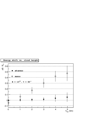
Figure 8: Energy and $x_{max}$ shift for 10²¹ eV showers with zenith angle $\theta=60^{o}$ as a function of cloud top height.

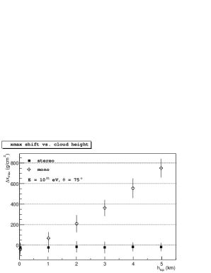
Figure 9: Energy and $x_{max}$ shift for showers with $\theta=75^{o}$and $E=10^{21}$eV. The x-axis is the cloud top height in km’s and the y-axis is $(E_{out}-E_{in})/E_{in}$.

Table 3: Energy shift (%) versus cloud height for shower energy of $10^{21}$ eV and shower zenith angle of 60^o. First column is cloud height in km. the following two are for stereo while the last two are for monocular.

$h_{top}$	stereo	$E$ shift	$x_{max}$ shift	mono	$E$ shift	$x_{max}$ shift
(km)	#events	%	g/cm2	#events	%	g/cm2
0	410	-0.4	-0.0	471	-4.6	-41.7
1	422	0.3	1.4	472	6.0	75.7
2	384	0.9	3.7	458	17.2	200.4
3	385	1.9	5.1	458	30.8	351.0
4	388	3.0	6.6	446	41.4	500.2
5	386	3.8	5.6	374	47.1	644.0

Table 4: Energy shift (%) versus cloud height for shower energy of $10^{21}$ eV and shower zenith angle of 75^o. First column is cloud height in km. the following two are for stereo while the last two are for monocular.

$h_{top}$	stereo	$E$ shift	$x_{max}$ shift	mono	$E$ shift	$x_{max}$ shift
(km)	#events	%	g/cm2	#events	%	g/cm2
0	411	-2.2	-3.3	469	-3.9	-21.7
1	411	-1.9	-3.5	470	5.9	101.7
2	419	-1.5	-1.3	461	16.5	240.3
3	391	-1.3	-3.6	454	28.0	389.1
4	229	-0.9	-1.0	254	40.7	553.5
5	400	-0.4	-1.2	293	53.1	727.5

The results show that while the performance of stereo is stable for different cloud heights, monocular reconstruction suffers badly if clouds at altitudes of 2 km or higher are present and their presence goes unrecognized. The reconstructed shower profiles in the monocular case “look” normal with the exception of the abnormal development depth and result in reasonable values for the $\chi^{2}$ as shown, for an example, in figure 10.

In case of stereo geometry, the last observed point along the shower track (pointing direction) can be converted to a position in space and therefore a height above the surface. This point can be interpreted as the surface height or cloud top height. Cloud presence can be identified by comparing this height with the known surface elevation. Figure 11 shows results from a test study. The cloud height is underestimated by approximately 0.5 km but the resolution is better than 0.5 km. In the figure, the error bars indicate the spread in the calculated heights and not the error on the mean.

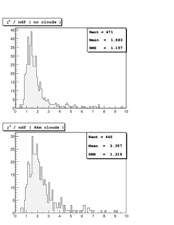
Figure 10: $\chi^{2}/ndf$ distribution from monocular reconstruction of two sets of showers: one set with no clouds, the other with clouds at 4 km. Showers were generated with a fixed energy of 10²¹ eV and a zenith angle of 60^o.

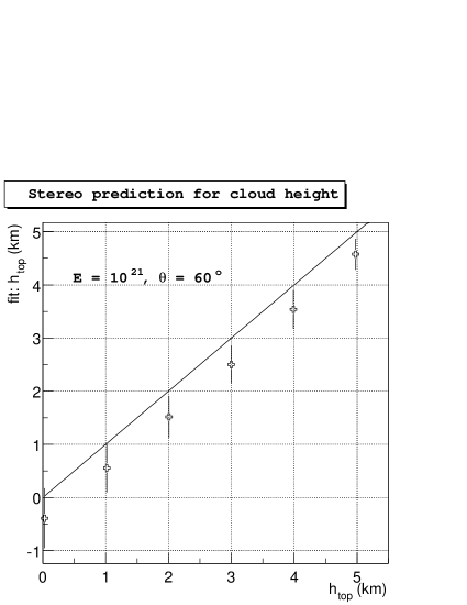
Figure 11: Stereo reconstruction of height of shower core, i.e., cloud height in case of reflection off opaque cloud. The cloud height is underestimated by approximately 0.5 km but the resolution is better than 0.5 km.

Appendix A Cloud Simulation

A.1 Introduction

The input parameters for the clouds model are: the cloud base height, $h_{base}$, the top height, $h_{top}$, and the vertical optical depth, $\tau$. The clouds density is uniform and falls to zero at the boundaries:

$$\rho_{c}=\left\{\begin{array}[]{cc}1&h_{base}<h<h_{top}\\ 0&otherwise\end{array}\right.$$

The vertical extent of the cloud, $\Delta z=h_{top}-h_{base}$, and the optical depth, $\tau$, determine the scattering coefficient through the relation $\tau=\beta\Delta z$. With $\beta$ given in 1/m. Note that $\sigma_{e}=\beta$ since we assume no absorption. The wavelength dependence of the cloud’s optical parameters is mild for $\lambda<0.5$ $\mu$m [18] and is ignored.

Several phase functions are relevant to a discussion of cloud scattering. The simplest is the Henyey-Greenstein (HG) phase function [29], given in eq. 15. It is often used in radiative transfer calculations as an analytic approximation to actual phase functions which may display complicated structures, see [30] and references therein.

$$P_{HG}(\cos(\theta_{s});g)=\frac{(1-g^{2})}{\left[1+g^{2}-2g\cos(\theta_{s})\right]^{3/2}}$$ (15)

Note that the parameter $g$ in the HG function is equal to the asymmetry parameter defined by:

$$g=\frac{1}{2}\int_{-1}^{1}P(\cos(\theta_{s}))\cos(\theta_{s})d\cos(\theta_{s})$$

where $\theta_{s}$ is the scattering angle and $P(\cos(\theta_{s}))$ is the phase function.

One feature of realistic clouds phase functions is a backward scattering peak. This feature is not reproduced by the HG function, however, a double-Henyey-Greenstein (DHG) function can provide a better fit, see fig. 12. The DHG function is defined by [31]:

$$P_{DHG}(g)=f\times P_{HG}(g_{1})+(1-f)\times P_{HG}(g_{2})$$

where $f\approx 1$ gives the forward scattering strength, and $g_{2}$ is negative.

Liou [19] gives in tabular form the phase function for a cirrostratus cloud model at a wavelength $\lambda=500$ nm. It is shown in figure 12 along with a HG and a DHG functions superimposed. A calculation of the asymmetry parameter for the realistic phase function gives $g=0.753$. The same value is used in the superimposed HG function. The DHG function parameters were set to: $g_{1}=0.82$, $g_{2}=-0.82^{2}$, and $f=0.96$.

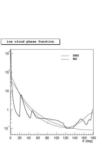
Figure 12: Ice clouds phase function (data from Liou at 0.5 $\mu$m .) A double Henyey-Greenstein approximation also shown.

A.2 Multiple Scattering in Clouds

A proper treatment of multiple scattering in clouds has to take into account the scattering and absorption by other atmospheric constituents. However, by considering the relative strength of the relevant processes, we can show that under certain conditions it is safe to ignore some of them. Thin cirrus clouds occur in the atmosphere at altitudes greater than 6 km and could be as high as 15 km. The extinction length varies with the clouds ice water content (determined in part by the altitude) and takes values on the order of a few kilometers. For comparison, extinction lengths due to molecular scattering, ozone absorption, and aerosols scattering are shown in figure 13.

Ozone absorption is negligible for wavelengths greater than $\lambda=320$ nm, and as can be seen from the figure, it can be safely dropped from the multiple scattering calculation for $\lambda>310$ nm. Aerosols density and extinction length are variable and whether or not they can be neglected depends on the local conditions. Figure 13 shows two examples, $L_{a}=10$ km, which represents a hazy atmosphere, and $L_{a}=23$ km, corresponding to an average atmosphere. Even in hazy conditions, the attenuation length due to aerosols is large for altitudes greater than 6 km because of the small scale height of the aerosols density distribution. For an average atmosphere, the aerosols extinction length is almost 20 times as large as the typical cloud extinction length, and can be safely neglected. Rayleigh scattering has a very strong wavelength dependence and can not be ignored at wavelengths close to $\lambda=300$ nm. For larger $\lambda$, and at altitudes greater than 6 km, the Rayleigh scattering length is greater than 20 km.

Figure 13: extinction length due to Rayleigh scattering, ozone absorption, and aerosols scattering as a function of altitude above sea level. U.S. 1976 standard atmosphere used for density profile for Rayleigh scattering.

A.2.1 An Isotropic Source

In this section we develop expressions for the direct transmission and transmission due to first, and second order scattering of light from a point source inside a cloud to a detector. First we define some notation. The point source is located at position $\vec{r}_{0}$, the detector (mirror) at $\vec{r}_{m}$. The points $\vec{r}_{1}$, $\vec{r}_{2}$ are the locations inside the cloud of first and second photon scattering respectively. The distance between any of the above points is denoted by $l_{ab}$ where $ab$ take the values of the subscripts of the respective points. In the case of the detector, we denote by $l_{am}$ the distance between $\vec{r}_{a}$ and $\vec{r}_{m}$ which lies inside the cloud, i.e. the path-length inside the cloud. the actual distance, $|\vec{r}_{m}-\vec{r}_{a}|$, is denoted by $R_{am}$. Direction and solid angle are denoted by $\Omega$. For example, $\Omega_{01}$ is the direction defined by the unit vector $(\vec{r}_{1}-\vec{r}_{0})/\left|\vec{r}_{1}-\vec{r}_{0}\right|$. The detector effective aperture is denoted by $A$, and the projected area of the detector with respect to $\vec{r}_{0}$ by $A_{\bot}^{(0)}$. The optical path length due to scattering by non-cloud particles (air, aerosols, or ozone absorption) is denoted by $\tau^{(nc)}$ with subscripts to identify the path. Non-clouds scattering and absorption coefficients are height dependent and so an integration over the path is required.

Let the point source emit isotropically $N_{s}$ photons, then the number of directly transmitted photons reaching the detector is given by:

$$N_{0}=\frac{N_{s}A_{\bot}^{(0)}}{4\pi R_{0m}^{2}}e^{-\beta_{c}l_{0m}}e^{-\tau_{0m}^{(nc)}}$$

First order scattering involves direct transmission to a point $\vec{r}_{1}$ then scattering in a volume element $dV_{1}$ into a solid angle $d\Omega$ at $\Omega$:

$$\frac{dN_{1}}{d\Omega}(\vec{r}_{1},\Omega)=\left(\frac{N_{s}\beta_{c}dV_{1}}{4\pi l_{01}^{2}}P(\Omega,\Omega_{01})e^{-\beta_{c}l_{01}}e^{-\tau_{01}^{(nc)}}\right)$$

where $P(\Omega,\Omega_{01})$ is the phase function for scattering by the cloud.

The number of photons received by the detector due to first order scattering taking attenuation along the path from $\vec{r}_{1}$ to the detector into account, is given by the integral over the cloud of:

$$dN_{1}=\frac{dN_{1}}{d\Omega}(\vec{r}_{1},\Omega_{1m})\times\left(\frac{A_{\bot}^{(1)}}{R_{1m}^{2}}e^{-\beta_{c}l_{1m}}e^{-\tau_{1m}^{(nc)}}\right)$$

The expression for second order scattering is similar to first order, however, instead of a point source at $\vec{r}_{0}$ we now have an integral over $\vec{r}_{1}$:

$$\frac{dN_{2}}{d\Omega}(\vec{r}_{2},\Omega) = \beta_{c}dV_{2}\int\frac{dN_{1}}{d\Omega}(\vec{r}_{1},\Omega_{12})$$

$$\times \frac{1}{l_{12}^{2}}P(\Omega,\Omega_{12})e^{-\beta_{c}l_{12}}e^{-\tau_{12}^{(nc)}}$$

The number of photons received by the detector is given by the integral of:

$$dN_{2}=\frac{dN_{2}}{d\Omega}(\vec{r}_{2},\Omega_{2m})\times\left(\frac{A_{\bot}^{(2)}}{R_{2m}^{2}}e^{-\beta_{c}l_{2m}}e^{-\tau_{2m}^{(nc)}}\right)$$

The evaluation of the above expressions and their integrals is done numerically, once a point source, a detector, and the cloud/atmosphere are specified.

A.2.2 Scattering out of a beam

Instead of an isotropic point source we now consider a light beam propagating in the direction, $\Omega_{0}$. Here we assume that $\Omega_{0}$ does not point toward the detector, i.e. the detector receives no direct light from the beam. Inside the cloud, light scattered out of the beam at a point $\vec{r}_{0}$ along the beam propagation path and into the detector is given by:

$$N_{1}=N_{s}P(\Omega_{0m},\Omega_{0})\times\left(\frac{A_{\bot}^{(0)}}{R_{0m}^{2}}e^{-\beta_{c}l_{0m}}e^{-\tau_{0m}^{(nc)}}\right)$$

where $N_{s}$ is the number of photons scattered out of the beam at the point $\vec{r}_{0}$.

Second order scattering inside the cloud is treated as follows: First consider light scattered out of the beam at $\vec{r}_{0}$ in some direction $\Omega_{01}$. At a point $\vec{r}_{1}$ along this direction, the irradiance is given by:

$$\frac{dN_{1}}{d\Omega_{01}}(\vec{r}_{1})=N_{s}P(\Omega_{01},\Omega_{0})e^{-\beta_{c}l_{01}}e^{-\tau_{01}^{(nc)}}$$

Next, the scattering in a volume element $dV_{1}$ at $\vec{r}_{1}$ into an arbitrary direction $\Omega$ is given by:

$$\frac{dN_{2}}{d\Omega}(\vec{r}_{1},\Omega)=\beta_{c}dV_{1}\left[\frac{dN_{1}}{d\Omega_{01}}(\vec{r}_{1})\right]P(\Omega,\Omega_{01})$$

Finally the contribution to the detector signal from the point $\vec{r}_{1}$ is:

$$dN_{2}=\frac{dN_{2}}{d\Omega}(\vec{r}_{1},\Omega_{1m})\times\left(\frac{A_{\bot}^{(1)}}{R_{1m}^{2}}e^{-\beta_{c}l_{1m}}e^{-\tau_{1m}^{(nc)}}\right)$$

The integral over the cloud volume of $dN_{2}$ gives the total contribution due to second order scattering of the beam photons inside the cloud.

A.2.3 Approximations

The OWL detector is located at an altitude of 800 km, this along with the fact that the scattering length inside the cloud is on the order of a few km’s, implies that: $R_{1m}\approx R_{0m}$ and $A_{\bot}^{(1)}\approx A_{\bot}^{(0)}$.These variables can then be taken out of the integrals and replaced by the approximate values.

The optical path length due to non-cloud scattering between two points, $\tau^{(nc)}$, requires an integration over the path joining the two points. A significant reduction in computation time can be achieved if appropriate approximations are used to replace these expressions which appear in the integrals by average values which can be taken out of the integrals. In the case of first order scattering we have: $\tau_{01}^{(nc)}$ and $\tau_{1m}^{(nc)}$. Given the strong forward peak of the scattering function we can see that the largest contribution to the integral comes from points close to the line joining the source and detector. This allows an approximation: $\bar{s}_{1}\approx\int dss\exp(-\beta_{c}s)/\int ds\exp(-\beta_{c}s)$ with the integration along the line segment from the source to the detector which is contained within the cloud. A vector position $<\vec{r}_{1}>$ can be defined using $\bar{s}_{1}$. Now $\tau_{1m}^{(nc)}$ will be replaced by an average value and taken out of the integral.

From the discussion at the beginning of this section we see that aerosols and ozone may be ignored in the volume of the cloud. Hence, $\tau_{01}^{(nc)}\approx\tau_{01}^{(R)}$, the optical depth due to Rayleigh scattering. The latter is given by $\int ds\beta_{R}(h)$ where $ds$ is along the line joining $\vec{r}_{0}$ and $\vec{r}_{1}$ and $h$ is the altitude along this line. In most cases of interest, the integral can be approximated by $|\vec{r}_{1}-\vec{r}_{0}|\times\beta_{R}(\bar{h})$, where $\bar{h}$ is the height of the midpoint between the two positions. This is due to the fact that the cloud thickness is on the order of one to a few km, less than the atmosphere scale height of $\sim 7$ km so $\beta_{R}$ does not change much along the integration path. This approximation was verified to be accurate to within 1-5% for a large number of test cases.

The strong wavelength dependence of Rayleigh scattering implies that the calculation should be repeated for each wavelength of interest. However, after considering a number of cloud configuration we saw that the result changes by less than 20% for wavelengths in the range of 337 nm, and 391 nm. We concluded that it would be a reasonable approximation to perform the calculation at a wavelength of $\lambda=357$ nm, and use the result as an average to be taken out of the sum over wavelengths.

Finally, after the calculation outlines in section A.2.2 was implemented for the shower’s Cerenkov beam, it became apparent that a simple alternative calculation which accounts for most of the additional signal received by the detector can be used instead. The strong forward peak of the cloud phase function results in that more than 52% of the photons scattered out of a beam are scattered forward in a cone of half-angle of 2^o. By not subtracting these photons from the beam, we in effect calculate the second order scattering of these photons at a later stage along the beam propagation when we evaluate the first order scattering from the beam at the later stage. The other 48% photons neglected in this approximation will have a lesser effect on the detector signal once one considers finite time window for the detector pixels.

A.3 Simple Cloud Monte Carlo

A simple method which works well and serves our needs is the Monte Carlo (MC) method. MC calculations are valid for clouds of all optical depths, however we only employ them for optically thick clouds. Currently our implementation only allows for clouds scattering but it can be easily extended to include Rayleigh and aerosols scattering. The calculation involves the following steps;

1. Select photon initial position inside the cloud or at a cloud boundary. Also, select the photon direction and a time offset relative to some $t_{0}$. The photon direction can be random, for isotropic distribution, or fixed in case of a beam.

2. Propagate the photon by a random step (distance) chosen from an exponential distribution: $\exp(-\beta_{c}l)$, with $\beta_{c}$ the extinction coefficient of the cloud

3. Check if new photon position is inside the cloud. If not then done, if it is then continue.

4. Select a random scattering angle drawn from a distribution which follows the clouds phase function. Select a uniform azimuthal angle. Set new photon direction.

5. Goto step 2

A simple “cloud MC” was developed around this algorithm to calculate the beam reflection from the top of a cloud. For a cloud with given cloud parameters a large number of photons impinging on the cloud top at a fixed angle (representing the beam’s zenith angle) is followed through the cloud. As the photons emerge from the cloud, either the cloud top (reflected) or cloud bottom (transmitted) they are added to a set of histograms which record the distributions of the locations and time delays of the photons. At the end of the run the histograms are saved to file and can be later used by the detector MC.

References

- [1] Y. Takahashi. Maximum-energy auger (air) shower satellite (mass) for observing cosmic rays in the energy region ev. In 24th ICRC, volume 3, pages 595–598, Rome, 1995.
- [2] J. F. Krizmanic, J. F. Ormes, and R.E. Streitmatter, editors. Workshop on Observing Giant Cosmic Ray Air Showers From eV Particles from Space, AIP Conference Proceedings 433, 1998. See also http://lheawww.gsfc.nasa.gov/docs/gamcosray /hecr/OWL/.
- [3] D. P. Wylie et al. Four years of global cirrus cloud statistics using hirs. Journal of Climate, 1994.
- [4] G. L. Cassiday et al. Measurnments of cosmic-ray air shower development at energies above ev. The Astrophysical Journal, 356:669–674, 1990.
- [5] L. Scarsi et al. Euso-extreme universe space observatory, a proposal for the esa f2/f3 missions. Technical report, ESA, 2000. See also http://www.euso-mission.org/.
- [6] K. N. Liou. Radiation and Cloud Processes in the Atmosphere, chapter 4. Oxford University Press, 1992.
- [7] C. L. Pryke. A comparitive study of the depth of maximum of simulated air shower longitudinal profiles. Astroparticle Physics, 14:319–328, 2001.
- [8] H. C. van de Hulst. Light Scattering by Small Particles, chapter 1. Dover Publications, Inc., 1981.
- [9] K.N. Liou et al. Laser transmission through thin cirrus clouds. Applied Optics, 39(27):4886–4894, 2000.
- [10] T. Abu-Zayyad et al. The prototype high-resolution fly’s eye cosmic ray detector. Nuclear Instruments & Methods in Physics Research A, 450:253–269, 2000.
- [11] T. Z. AbuZayyad. The Energy Spectrum of Ultra High Energy Cosmic Rays. PhD thesis, University of Utah, 2000.
- [12] Rene Brun and Fons Rademakers. Root - an object oriented data analysis framework. Nuclear Instruments & Methods in Physics Research A, 389:81–86, 1997. See also http://root.cern.ch/.
- [13] J. F. Krizmanic et al. Owl roadmap to the ultra-high-energy universe. Technical report, NASA, 2002.
- [14] U.S. Standard Atmosphere, 1976. U.S. Government Printing Office, Washington, D.C., 1976.
- [15] R. M. Baltrusaitis et al. The utah fly’s eye detector. Nuclear Instruments and Methods in Physics Research, A240:410–428, 1985.
- [16] D. R. Longtin. A wind dependent aerosol model: Radiative properties. Technical Report AFGL-TR-88-0112, Air Force Geophysics Laboratory, 1988.
- [17] USAF Air Force Geophysics Laboratory. Handbook of Geophysics and the Space Environment, 1985.
- [18] K. N. Liou. Radiation and Cloud Processes in the Atmosphere, chapter 5, pages 267,275. Oxford University Press, 1992.
- [19] K. N. Liou. Radiation and Cloud Processes in the Atmosphere, chapter 5, page 276. Oxford University Press, 1992.
- [20] T. K. Gaisser and A. M. Hillas. In 15th ICRC, volume 8, page 353, Plovdiv, 1977.
- [21] John Linsley. In 18th ICRC, volume 12, page 135, Bangalore, 1983.
- [22] C. Song et al. Energy estimation of uhe cosmic rays using the atmospheric fluorescence technique. Astroparticle Physics, 14:7–13, 2000.
- [23] D. J. Bird et al. Evidence for correlated changes in the spectrum and composition of cosmic rays at extremely high energies. Physical Review Letters, 71(21):3401–3404, 1993.
- [24] K. Kamata and J. Nishimura. Progress in Theoretical Physics Supplement, 6:93, 1958.
- [25] K. Greisen. Annual Review of Nuclear Science, 10:63, 1960.
- [26] F. Kakimoto et al. A measurement of the air fluorescence yield. NIM A, 372, 1996.
- [27] C. R. Wilkinson et al. Geometrical reconstruction with the high resolution fly’s eye prototype cosmic ray detector. Astroparticle Physics, 12(3):121–134, 1999.
- [28] Paul Sommers. Capabilities of a giant hybrid air shower detector. Astroparticle Physics, 3:349–360, 1995.
- [29] L. C. Henyey and J. L. Greenstein. Diffuse radiation in the galaxy. The Astrophysical Journal, 93:70–83, 1941.
- [30] Olivier Boucher. On aerosol direct shortwave forcing and the henyey-greenstein phase function. Journal of the Atmospheric Sciences, 55:128–134, 1998.
- [31] Richard L. White. Polarization in reflection nebulae. i. scattering properties of interstellar grains. The Astrophysical Journal, 229:954–961, May 1979.