X–ray properties of galaxy clusters and groups from a cosmological hydrodynamical simulation

Abstract

We present results on the X–ray properties of clusters and groups of galaxies, extracted from a large cosmological hydrodynamical simulation. We used the Tree+SPH code GADGET to simulate a concordance $\Lambda$CDM cosmological model within a box of $192\,h^{-1}{\rm Mpc}$ on a side, $480^{3}$ dark matter particles and as many gas particles. The simulation includes radiative cooling assuming zero metallicity, star formation and supernova feedback. The very high dynamic range of the simulation allows us to cover a fairly large interval of cluster temperatures. We compute X–ray observables of the intra–cluster medium (ICM) for simulated groups and clusters and analyze their statistical properties. The simulated mass–temperature relation is consistent with observations once we mimic the procedure for mass estimates applied to real clusters. Also, with the adopted choices of $\Omega_{m}=0.3$ and $\sigma_{8}=0.8$ for matter density and power spectrum normalization, respectively, the resulting X–ray temperature function agrees with the most recent observational determinations. The luminosity–temperature relation also agrees with observations for clusters with $T\raise-2.0pt\hbox{\hbox to0.0pt{\hbox{$\sim$}\hss}\raise 5.0pt\hbox{$>$}\ }2$ keV. At the scale of groups, $T\raise-2.0pt\hbox{\hbox to0.0pt{\hbox{$\sim$}\hss}\raise 5.0pt\hbox{$<$}\ }1$ keV, we find no change of slope in this relation. The entropy in central cluster regions is higher than predicted by gravitational heating alone, the excess being almost the same for clusters and groups. We also find that the simulated clusters appear to have suffered some overcooling. We find $f_{*}\simeq 0.2$ for the fraction of baryons in stars within clusters, thus about twice as large as the value observed. Interestingly, temperature profiles of simulated clusters are found to steadily increase toward cluster centers. They decrease in the outer regions, much like observational data do at $r\raise-2.0pt\hbox{\hbox to0.0pt{\hbox{$\sim$}\hss}\raise 5.0pt\hbox{$>$}\ }0.2\,r_{\rm vir}$, while not showing an isothermal regime followed by a smooth temperature decline in the innermost regions. Our results thus demonstrate the need for yet more efficient sources of energy feedback and/or the need to consider additional physical process which may be able to further suppress the gas density at the scale of poor clusters and groups, and, at the same time, to regulate the cooling of the ICM in central regions.

1 Introduction

Observations of galaxy clusters in the X–ray band offer a unique means to study the physical properties of the diffuse cosmic baryons in the intra–cluster medium (ICM; see Sarazin 1988, for a historical review). Under the action of gravity, these baryons follow the dark matter during the process of hierarchical structure formation, in which they are heated by adiabatic compression during the halo mass growth and by shocks induced by supersonic accretion or merger events. Since gravity does not have any preferred scale, clusters and groups are in principle expected to appear as scaled version of each other, provided gravity dominates the process of gas heating (Kaiser 1986) and the power spectrum of primordial perturbations is featureless over the relevant scales. Under the additional assumptions that gas is in hydrostatic equilibrium within the dark matter (DM) potential wells and that bremsstrahlung dominates the emissivity, this scenario predicts self–similar X–ray scaling relations for cluster and group properties: (i) $L_{X}\propto T^{2}$ for the relation between X–ray luminosity and gas temperature; and (ii) $M_{\rm gas}\propto M_{\rm vir}\propto T^{3/2}$ for the relation between gas mass, total virialized mass and temperature. Furthermore, if we define the gas entropy as $S=T/n_{e}^{2/3}$, then the self–similarity of gas density profiles leads to the scaling $S\propto T$ if entropy is estimated at a fixed overdensity for different clusters. The overall validity of these scaling relations has been confirmed by hydrodynamical simulations of galaxy clusters that included only gravitational heating (e.g., Navarro, Frenk & White 1995; Evrard, Metzler & Navarro 1996; Bryan & Norman 1998; Eke, Navarro & Frenk 1998).

However, a variety of observational evidences demonstrates that this simple picture does not apply to real clusters. The luminosity–temperature relation is observed to be steeper than predicted, $L_{X}\propto T^{\alpha}$, with $\alpha\simeq 2.5$–3 for clusters with $T>2$ keV (e.g., White, Jones & Forman 1997; Markevitch 1998; Arnaud & Evrard 1999; Ettori, De Grandi & Molendi 2002), with indications of an even steeper slope at the scale of groups, $T\raise-2.0pt\hbox{\hbox to0.0pt{\hbox{$\sim$}\hss}\raise 5.0pt\hbox{$<$}\ }1$ keV (e.g., Ponman et al. 1996; Helsdon & Ponman 2000; Sanderson et al. 2003; cf. Mulchaey & Zabludoff 1998, and Osmond & Ponman 2003). In addition, the evolution of this relation appears to be slower than predicted by self–similarity (e.g., Holden et al. 2002; Novicki, Sornig & Henry 2002; Ettori et al. 2003, and references therein) although this result is still a matter of debate (e.g., Vikhlinin et al. 2002). Also, the relation between gas mass and temperature is observed to be steeper than the self–similar one, $M_{\rm gas}\propto T^{\alpha}$, with $\alpha\simeq 1.7$–2.0 (e.g., Mohr, Mathiesen & Evrard 1999; Vikhlinin, Forman & Jones 1999; Neumann & Arnaud 1999; Ettori et al. 2002b), or, equivalently, poor clusters and groups contain a relatively smaller amount of gas (e.g., Sanderson et al. 2003, and references therein). Finally, the gas entropy within clusters is in excess with respect to what is expected from self–similar scaling (e.g., Ponman, Cannon & Navarro 1999; Lloyd–Davies, Ponman & Cannon 2000; Finoguenov et al. 2002), with a dependence on temperature roughly equal to $S\propto T^{2/3}$ (Ponman, Sanderson & Finoguenov 2003).

These observational results indicate that non–gravitational processes that took place during cluster formation must have substantially affected the physics of the ICM and left an imprint on its X–ray properties. A variety of models have been developed so far to explain the resulting ICM properties and, in particular, the lack of self–similarity between clusters and groups. These models can be broadly classified into two categories: those which are based on non–gravitational heating processes of the ICM (e.g., Evrard & Henry 1991; Kaiser 1991; Bower 1997; Cavaliere, Menci & Tozzi 1998; Balogh, Babul & Patton 1999; Tozzi & Norman 2001; Babul et al. 2002), and those which resort on the effects of radiative cooling (e.g., Bryan 2000; Voit & Bryan 2001; Wu & Xue 2002; Voit et al. 2002).

Non–gravitational heating increases the entropy of the gas, which can prevent it from reaching high density during the cluster collapse. If a given amount of heating energy per particle, say $E_{h}$, is assigned to the gas, then we expect the effect of extra heating to be negligible for massive clusters with virial temperature $T>E_{h}$, while it should leave a significant imprint on smaller systems with $T\raise-2.0pt\hbox{\hbox to0.0pt{\hbox{$\sim$}\hss}\raise 5.0pt\hbox{$<$}\ }E_{h}$. As a consequence, X–ray luminosity and gas mass are suppressed by a larger amount in smaller systems, thus causing a steepening of the $L_{X}$–$T$ and $M_{\rm gas}$–$T$ relations. Furthermore, extra heating also sets a minimum value for the entropy that gas can reach in central regions of clusters and groups, which can in principle account for the observed excess. In fact, both semi–analytical models (e.g., Balogh et al. 1999; Tozzi & Norman 2001) and numerical simulations (e.g., Bialek et al. 2001; Brighenti & Mathews 2001; Borgani et al. 2001a, 2002) were able to demonstrate that observational data can be reproduced by assigning a heating energy of about 0.5–1 keV per particle or, equivalently, by imposing a pre–collapse entropy floor of $S_{\rm fl}\sim 50$–100 keV cm².

As for the origin of extra–heating, supernovae (SN) have been considered as a first possibility (e.g., Menci & Cavaliere 2000; Bower et al. 2001). Using the metal content of the ICM as a diagnostic for the number of SN exploded (e.g., Renzini 1997, 2003; Kravtsov & Yepes 2000; Finoguenov, Arnaud & David 2001; Pipino et al. 2002), several authors concluded that SN may however not be able to supply the required amount of feedback energy. A pristine, essentially metal-free stellar population, the so–called Pop-III stars, has also been suggested to contribute significantly to pre–heating (Loewenstein 2001), although their contribution is constrained by the requirement of not to over–heat and over–pollute the high–redshift intergalactic medium (IGM; Scannapieco, Schneider & Ferrara 2003). Another possible source for ICM heating is represented by AGN (e.g, Valageas & Silk 1999; Wu, Fabian & Nulsen 2000; Mc Namara et al. 2000; Cavaliere, Lapi & Menci 2002). In this case, the available energy budget is in principle quite large, but a coherent treatment of the conversion of mechanical energy of jets into thermal energy of the diffuse medium (Reynolds, Heinz & Begelman 2002; Omma et al. 2003) is still missing.

Although it may sound like a paradox, radiative cooling has also the effect of increasing the entropy of the diffuse cluster baryons. This results as a consequence of the selective removal of low–entropy gas, which is characterized by a cooling time shorter than the typical cluster age (e.g., Voit & Bryan 2001; Wu & Xue 2002). Besides increasing the observed mean entropy, the removal of gas from the X–ray emitting phase also reduces the X–ray luminosity (e.g., Muanwong et al. 2002; Davé et al. 2002), much like in the heating scenario. Although cooling must clearly occur at some level as soon as gas reaches high density within collapsed halos, it has the unpleasant feature to be a runaway process. This manifests itself in numerical simulations that include gas cooling and star formation, but no efficient heating processes. These simulations invariably find that a very large fraction $f_{*}$ of gas is converted into a “stellar” cold medium, with $f_{*}\raise-2.0pt\hbox{\hbox to0.0pt{\hbox{$\sim$}\hss}\raise 5.0pt\hbox{$>$}\ }30$ per cent (e.g., Suginohara & Ostriker 1998; Lewis et al. 2000; Yoshida et al. 2002; Tornatore et al. 2003), which lies substantially above typical observed values, $f_{*}\raise-2.0pt\hbox{\hbox to0.0pt{\hbox{$\sim$}\hss}\raise 5.0pt\hbox{$<$}\ }10$ per cent (e.g., Balogh et al. 2001; Lin, Mohr & Stanford 2003), derived from the local luminosity density of stars.

This demonstrates the need to develop a more realistic and self–consistent description of the ICM where the effect of cooling is counteracted and regulated by energy feedback from astrophysical sources (e.g., Oh & Benson 2003). In this spirit, Voit et al. (2002) have developed a semi–analytical framework which includes the combined effect of cooling and extra heating. While cooling is responsible for setting the level of the entropy floor in this model, extra heating regulates the amount of gas which lies above the entropy limit for the onset of cooling. However, combining heating and cooling in a dynamically self–consistent way has been not achieved yet. Hydrodynamical simulations of clusters including cooling and different models for non–gravitational heating (Tornatore et al. 2003) have shown that these two effects interact with each other in a non–trivial way and, in general, it is not at all obvious that they can be combined such that overcooling is avoided while simultaneously providing a good fit to the X–ray scaling relations.

As the level of complexity in the description of the ICM physics is increased, hydrodynamical simulations are becoming invaluable theoretical tools to keep pace with the observational progress brought about by the unprecedented quality of X–ray data from the Chandra and XMM–Newton satellites. However, an important factor limiting the reliability of numerical simulations is given by their numerical resolution, which is usually determined by a combination of the available supercomputing time and the simulation code’s capabilities. For this reason, numerical studies of the ICM typically represent a compromise between the mass resolution that one wants to achieve within each single cluster–sized halo and the number of clusters and groups that one wants to study numerically. Finding an optimal compromise is not easy when one is interested in X–ray studies of clusters. On one hand, the dependence of the bremsstrahlung emissivity on the density squared requires that small–scale details of the gas distribution are correctly represented, otherwise the simulated X-ray emissivity will be incorrect. On the other hand, a reliable comparison with observational results on cluster X–ray scaling relations requires a statistically representative ensemble of halos to be simulated, which can only be obtained in a large simulation volume, at the price of compromising the mass-resolution.

Hydrodynamical simulations of individual cluster–sized halos, based on zoom–in resimulation techniques (e.g., Katz & White 1993; Tormen, Bouchet & White 1997), presently allow each object to be represented with $\sim 10^{5}$ particles, with a force resolution of about 5 $h^{-1}$kpc (e.g., Borgani et al. 2002; Valdarnini 2003; Tornatore et al. 2003; Tormen, Moscardini & Yoshida 2003). On the other hand, simulations of cosmological boxes, with sizes ranging from about 50 up to few hundreds $\,h^{-1}{\rm Mpc}$ on a side, have been run with the purpose of simulating in one realization a statistically representative number of clusters and groups (e.g., Bryan & Norman 1998; Muanwong et al. 2002; Bond et al. 2002; Davé et al. 2002; Zhang, Pen & Wang 2002; White, Hernquist & Springel 2003; Springel & Hernquist 2003b; Motl et al. 2003). For example, Muanwong et al. (2002) analysed X–ray properties of clusters and groups in simulations with a box–size of 100$\,h^{-1}{\rm Mpc}$ containing $2\times 160^{3}$ DM and gas particles, with gravitational softening of a few tens $h^{-1}$ kpc. In order to achieve a better mass and force resolution, Davé et al. (2002) and Kay et al. (2003) adopted a smaller box size of 50$\,h^{-1}{\rm Mpc}$ with $2\times 144^{3}$ and $2\times 128^{3}$ gas and DM particles, respectively, thus restricting themselves to the study of galaxy groups; rich clusters are not found in such small volumes. While these simulations were based on the SPH technique, Motl et al. (2003) used an Eulerian code capable of adaptive mesh refinement (AMR) to simulate a cosmological box of 256$\,h^{-1}{\rm Mpc}$ on a side, reaching a mass resolution of about $10^{10}h^{-1}M_{\odot}$ at their highest refinement level. This simulation included radiative cooling, but neglected the effect of SN feedback.

In this paper, we present results on the X–ray properties of clusters and groups identified in a new, very large SPH simulation within a cosmological box of size 192$\,h^{-1}{\rm Mpc}$ on a side, using $480^{3}$ DM particles and as many gas particles. The simulation includes radiative cooling, a prescription for star formation in a multi–phase model for the interstellar medium (ISM), and a recipe for galactic winds triggered by SN explosions, as described in full detail by Springel & Hernquist (2003a). Thanks to the force and mass resolution achieved, we resolve galaxy groups, having a temperature of about 0.5 keV, with $\sim 5000$ gas particles, while the most massive halos found in the box have $\sim 10^{5}$ gas particles within the virial radius. This simulation hence combines fairly high resolution in a large cosmological volume with a quite advanced treatment of the gas physics. It is thus ideally suited for a comparison between simulated and observed X–ray properties of groups and clusters, allowing us to shed more light on the interplay between the properties of the ICM and the processes of star formation in cluster galaxies.

The outline of the paper is as follows. In Section 2, we describe the numerical method that we use, and provide an overview of the general characteristics of the simulation. Section 3 is devoted to the presentation of the results. After discussing the star fraction produced within the cluster regions, we study the different X–ray observables, such as luminosity, temperature and entropy. Much emphasis will be given through all of this section to a comparison of the numerical results with X–ray observations. Finally, we summarize our results and draw our main conclusions in Section 4.

2 The simulation

The cosmological model we simulated represents a standard flat $\Lambda$CDM universe, with matter density $\Omega_{m}=0.3$, Hubble constant $H_{0}=70$ km s^-1Mpc^-1, baryon density $\Omega_{\rm bar}=0.04$ and normalization of the power spectrum $\sigma_{8}=0.8$. This normalization is somewhat lower, though consistent within 1$\sigma$, than suggested by the WMAP result (Spergel et al. 2003), but it is consistent with recent determinations based on the number density of galaxy clusters (e.g., Pierpaoli et al. 2003, and references therein), or based on cosmic shear measurements (see Refregier 2003, for a review). The baryon density agrees with the prediction of big–bang nucleosynthesis for the deuterium abundance found in high–$z$ Lyman–$\alpha$ clouds by Kirkman et al. (2003), while it is $\simeq 20$ per cent lower, though consistent at about $1\sigma$ level, with the WMAP value.

Initial conditions have been generated at redshift $z_{\rm start}\simeq 46$ within a box of $192\,h^{-1}{\rm Mpc}$ on a side using the COSMICS package provided by E. Bertschinger. The density field has been sampled with $480^{3}$ dark matters and an equal number of gas particles, with masses of $m_{\rm DM}=6.6\times 10^{9}M_{\odot}$ and $m_{\rm gas}=9.9\times 10^{8}M_{\odot}$, respectively. For our choices of starting redshift and mass resolution, the rms Zeldovich displacement in the initial conditions was equal to about one tenth of the mean interparticle separation. During the evolution, the number of gas particles changes as a consequence of their partial conversion into new star particles. Because the generated star particles have mass smaller than gas particles, the total number of particles actually increases by a small amount as a result of star formation.

The run has been realized using GADGET, a massively parallel tree N–body/SPH code (Springel, Yoshida & White 2001) with fully adaptive time–step integration. We here used GADGET-2, a new version of this simulation code that is more efficient than earlier versions of GADGET, and offers better time–stepping for collisionless dynamics, among other improvements. Of particular relevance is the implementation of SPH adopted in the code, which follows the formulation suggested by Springel & Hernquist (2002). This method explicitly conserves energy and entropy, where appropriate, and substantially reduces numerical overcooling problems at interfaces between hot and cold gas. Optionally, the new code also allows the use of a TreePM algorithm (Bagla 2002) to speed up the computation of the long-range gravitational force, an approach that we employed in the present simulation.

Radiative cooling was computed assuming an optically thin gas of primordial composition (mass–fractions of $X=0.76$ for hydrogen and $1-X=0.24$ for helium) in collisional ionization equilibrium, following Katz, Weinberg & Hernquist (1996). We have also included a photoionizing, time–dependent, uniform UV background expected from a population of quasars (e.g., Haardt & Madau 1999), which reionizes the Universe at $z\simeq 6$. The effect of a photoionizing background is that of inhibiting gas collapse and subsequent star formation within the halos of sub–$L_{*}$ galaxies (e.g., Benson et al. 2002), thus having a secondary impact at the resolution of our simulation. Although the code includes a method to follow metal production (see below), we have not included the effects of metals on the cooling function, owing both to code limitations and to the approximate treatment of metal generation and diffusion.

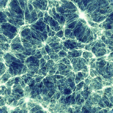
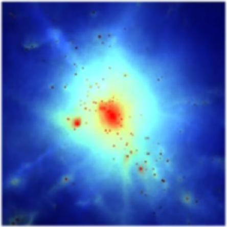
Figure 1: Left panel: map of the gas density over the whole simulation box at $z=0$, projected using a ray–tracing technique through a slice having thickness of 12 $\,h^{-1}{\rm Mpc}$, and containing the most massive cluster found in the simulation (upper right side of the panel). Right panel: zoom into the region of the largest cluster; the cluster is shown out to one virial radius, so that the panel encompasses a physical scale of about 4.5 $h^{-1}$ Mpc.

Star formation is treated using the hybrid multiphase model for the interstellar medium introduced by Springel & Hernquist (2003a). We refer to this paper for a detailed description of the method, providing here only a short summary of the model. The ISM is pictured as a two-phase fluid consisting of cold clouds that are embedded at pressure equilibrium in an ambient hot medium. The clouds form from the cooling of high density gas, and represent the reservoir of baryons available for star formation. When stars form, according to a Salpeter IMF (Salpeter 1955), the energy released by supernovae heats the ambient hot phase of the ISM, and in addition, clouds in supernova remnants are evaporated. These effects establish a tightly self–regulated regime for star formation in the ISM. In practice, the scheme is numerically implemented as a sub-resolution model, i.e. cold clouds are not resolved individually. Instead, only their total mass fraction in each element of the ISM is computed, otherwise they are treated in a stochastic fashion with their collective effect on the ISM dynamics being described by an effective equation of state. The numerical implementation of this multiphase model describes each gas particle as composed by a hot component, having its own mass and density, and a cold neutral component. The relative amount of these two phases is determined by the local value of gas density and temperature. We note that metal enrichment and type-II supernovae feedback is computed assuming an instantaneous recycling approximation.

If not counteracted by some sort of feedback process, cooling is well known to overproduce the amount of stars both in the average environment and in the group/cluster overdense environment (e.g. Balogh et al. 2001, and references therein). As discussed by Springel & Hernquist (2003a), their multiphase ISM model alone does however not fully resolve this problem, despite its ability to regulate the consumption of cold gas into stars within the ISM. This is because the cooling rates within halos remain essentially unaffected in the model, i.e. the supply of gas to the dense star-forming ISM is largely unchanged, while by construction the phases of the ISM remain coupled to each other, preventing baryons to leave the ISM (except for dynamical effects like gas stripping in mergers).

However, galactic outflows are observed and expected to play a key role in transporting energy and metals produced by the stellar population into the IGM/ICM. To account for them, Springel & Hernquist (2003a) suggested a phenomenological description of galactic winds as an extension of their model, and we have included such winds in our simulation. According to our choice of parameters for the feedback and wind scheme, star-forming gas particles contribute to the wind with a mass outflow rate two times larger than their star formation rate, with a wind velocity of about $360\,{\rm km\,s^{-1}}$. This velocity is less extreme than the value of about $480\,{\rm km\,s^{-1}}$ adopted by Springel & Hernquist (2003b) in their comprehensive study of the cosmic star formation history. In fact, the energy of our winds is only half that of Springel & Hernquist (2003b), who assumed that essentially all of the feedback energy is available to power the winds. With this choice, Springel & Hernquist (2003b) were able to show that the global efficiency of cooling and star formation is reduced to the observed level, and that observational constraints on the amount of neutral hydrogen in high column–density absorbing systems at high redshift (Nagamine, Springel & Hernquist 2003a,b) can be accounted for. However, we preferred here a more conservative choice of less energetic winds, so as to allow for radiative losses taking place in the interstellar medium at sub–resolution scales.

The Plummer–equivalent gravitational softening of the simulation was set to $\epsilon_{\rm Pl}=7.5\,h^{-1}$ kpc comoving from $z=2$ to $z=0$, while it was taken to be fixed in physical units at higher redshift. We used 32 neighboring particles for the SPH computations, but did not allow the SPH smoothing length to drop to less than one quarter of the value of the gravitational softening length of the gas particles. In total, the simulation required about 40,000 CPU hours on 64 processors of the IBM-SP4 machine located at CINECA. We produced 100 snapshots at log-equispaced values of the expansion factor, from $a_{\rm exp}=0.1$ to $a_{\rm exp}=1$, thus producing a total amount of about 1.2 Tb of data. The fine spacing of snapshots in time can be used to measure merger tree of halos, and to realize projections along the backward light–cone.

3 Results

We start our analysis with an identification of groups and clusters within the simulations box. To this end, we first apply a friends-of-friends halo finder to the distribution of DM particles, with a linking length equal to 0.15 times their mean separation. For each group of linked particles with more than 500 members, we identify the particle having the minimum value of the gravitational potential. This particle is then used as a starting point to run a spherical overdensity algorithm, which determines the radius around the target particle that encompasses an average density equal to the virial density for the adopted cosmological model, $\rho_{\rm vir}(z)=\Delta_{c}(z)\rho_{c}(z)$, where $\rho_{c}(z)=[H(z)/H_{0}]^{2}\rho_{c,0}$ is the critical density at redshift $z$, and the overdensity $\Delta_{c}(z)$ is computed as described in Eke, Cole & Frenk (1996).

In the left panel of Figure 1, we show a map of the gas distribution at $z=0$, projected through a slice of thickness 1/16th of the box size. This slice includes the most massive cluster found in the simulation, which is located in the upper right region of the map. The panel on the right shows the gas distribution of this cluster out to the virial radius, thus representing a zoom-in by about a factor of 40. The tiny dark spots visible in the central cluster regions are condensations of high–density cold gas. They mark the locations where star formation is taking place and, therefore, the positions of cluster galaxies. The amount of small–scale detail which is visible in the zoom–in of the right panel demonstrates the large dynamic range encompassed by the hydrodynamic treatment of the gas in our simulation.

The cluster shown in Fig. 1, which has an emission–weighted temperature of $T_{\rm ew}\simeq 7\,{\rm keV}$ (see below), is resolved with about $2\times 10^{5}$ DM particles within the virial radius. Overall, we have 400 halos resolved with at least 10,000 DM particles, 72 clusters with $T_{\rm ew}>2$ keV, out of which 23 have $T_{\rm ew}>3$ keV. Clusters with $T_{\rm ew}=1$ keV are resolved with about 7,000 DM particles. Therefore, our simulation provides us with an unprecedented large sample of simulated groups and clusters of medium-to-low richness that are represented with good enough numerical resolution to obtain reliable estimates of X–ray observable quantities, such as luminosity, temperature and entropy.

In the following, we will mainly concentrate on the description of the properties of clusters at $z=0$, while we will deserve to a forthcoming paper the discussion of the redshift evolution of the X–ray scaling relations and their comparison with observational data.

3.1 The stellar fraction in clusters

Observational determinations of the fraction of baryons locked up in stars in galaxy clusters, $f_{*}$, consistently indicate a rather small value. For instance, Balogh et al. (2001) found this fraction to be below 10 per cent, independent of the cluster richness. More recently, Lin et al. (2003) selected a sample of nearby clusters, with ICM masses available from ROSAT-PSPC data and total stellar mass estimated from the total K–band luminosity, as provided by the 2MASS survey (e.g., Cole et al. 2001). They found that rich clusters have $f_{*}\raise-2.0pt\hbox{\hbox to0.0pt{\hbox{$\sim$}\hss}\raise 5.0pt\hbox{$<$}\ }10$ per cent, with an increasing trend toward poorer systems (see the data points plotted in Figure 2).

On the other hand, hydrodynamical simulations of clusters that include radiative cooling and star formation, have demonstrated that significantly higher $f_{*}$ values, as high as 30–50 per cent, are found when sufficiently high numerical resolution is adopted (e.g., Balogh et al. 2001; Davé et al. 2002; Tornatore et al. 2003). This reflects the well established result that radiative cooling converts a large fraction of baryons into collisionless stars (e.g., Suginohara & Ostriker 1998; Balogh et al. 2001) if it is not efficiently counteracted by some sort of feedback process that heats the gas surrounding star–forming regions, thus increasing its cooling time and preventing a “runaway” overcooling.

While consistency with the observed $f_{*}$ values can eventually be reached by adopting suitable schemes for gas pre–heating and feedback (e.g., Muanwong et al. 2002; Kay et al. 2003; Tornatore et al. 2003; Marri & White 2003), it is not trivial at all to implement such schemes in a numerically self–consistent and physically well motivated way within cosmological simulations of structure formation. Note that feedback energy associated with star formation is most plausibly released in star–forming regions, where gas is at high density and, therefore, has short cooling time. Increasing the thermal energy of this gas is hence quite ineffective in preventing it from cooling. For this reason, a physically motivated model for either preventing such particles from radiating away the heating energy or for assigning this energy to particles at lower density (which have longer cooling times) is needed.

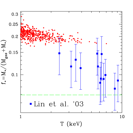
Figure 2: The fraction of gas locked into stars, estimated at the virial radius from simulations (small circles) and from observational data (big squares with errorbars; from Lin et al. 2003). The horizontal dashed line indicates the cosmic value of $f_{*}$ found in the simulation.

The feedback model by Springel & Hernquist (2003a) included in our simulation represents a simple physical model of the expected multi-phase structure of the ISM. This model has well-controlled numerical properties, in the sense that the star formation rate in a given halo converges even at moderate numerical resolution, which is desirable for simulations of hierarchical structure formation. The modelization of galactic winds accounts for the role of galactic ejecta, and is crucial for transferring SN energy out of the star–forming environment itself. If strong winds are adopted, this feedback scheme is in fact able to reproduce the observed cosmic star–formation history and to reduce the total amount of baryons to about 10 per cent.

However, in our simulation a somewhat weaker wind model was adopted (see the discussion in Section 2). With this choice, the total mean cosmic value of $f_{*}\simeq 7$ per cent of stars produced in the simulation is consistent with observational results (e.g., Fukugita, Hogan & Peebles 1998; Balogh et al. 2001), although such a low value may be due to the lack of objects below our resolution limit. At the same time, the efficiency of star formation within the high–density environment of clusters is still in excess with respect to observations. Values of $f_{*}$ for individual clusters are at the level of $\simeq 20$ per cent for $T>3$ keV clusters, with a slight tendency to increase for colder systems, as shown in Figure 2.

As a word of caution, it is important to be aware of the resolution limitations of our simulation. The necessity of keeping the box–size large enough for our study compromises its mass resolution, even for the fairly large number of particles followed in this run. This is particularly important in the context of feedback by galactic winds. Whether or not ejecta can escape the gravitational potential of a galaxy depends primarily on its virial mass: while it is relatively easy for a wind to escape from small objects, winds are expected to provide only inefficient feedback in massive galaxies and halos, where they are confined gravitationally. Since we can hardly treat the effect of winds on unresolved, or poorly resolved, small galaxies, we may be underestimating the effect of winds on our smallest systems. This is particularly true at high redshift, when large numbers of small halos start collapsing. In addition, we miss the cumulative effect of winds during the hierarchical built-up of structure up to the point where we start resolving massive enough objects. This could result in an underestimate of the degree of metal dispersal estimated from the simulation, for example. While we are not carrying out detailed resolution studies ourselves, these are ultimately needed to fully eliminate these uncertainties. However, we note that the star formation rate of well resolved objects is expected have converged in our simulation, as demonstrated by Springel & Hernquist (2003b) for the same feedback model and simulation code used here.

3.2 Computing X–ray luminosity and temperature

Since the simulation adopts a zero–metallicity cooling function, we accordingly compute X–ray emissivity under this assumption. Therefore, the resulting X–ray luminosity of each cluster in a given energy band is defined as

$$L_{X}\,=\,(\mu m_{p})^{-2}\sum_{i}^{N_{\rm gas}}m_{h,i}\rho_{h,i}\Lambda(T_{i}),$$ (1)

where $\Lambda(T)$ is the cooling function in that energy band. In this equation the sum runs over all $N_{\rm gas}$ gas particles falling within $r_{\rm vir}$, and $\mu$ is the mean molecular weight ($=0.6$ for a gas of primordial composition), $m_{p}$ is the proton mass, $m_{h,i}$ and $\rho_{h,i}$ are the mass and the density associated with the hot phase of the $i$–th gas particle, respectively. A distinction between hot and cold phases is only made for dense star-forming particles, where the adopted multiphase model allows a computation of the relative contribution of each of these two phases, which depends on the local density and temperature (Springel & Hernquist 2003a). By its nature, the neutral cold component is assumed to not emit any X–rays. In addition, we also exclude those particles from the computation of X–ray emissivity whose ionized component has temperature below $3\times 10^{4}$ K and density $>500\rho_{c}(z)$. Particles inside clusters at such low temperature are usually at very high density (often they are particles just assigned to the wind by the phenomenological wind model), much higher than the threshold chosen above. As such, they would provide a significant, but spurious, contribution to the X–ray luminosity in central cluster regions if they were X–ray emitting. These particles occupy a region in the $\rho$–$T$ plane where in principle only gas should lie that has already cooled, and so this gas should not be included in the computation of the X–ray emission (Croft et al. 2001; Kay et al. 2002).

For the cooling function, we assumed the one provided by Sutherland & Dopita (1993), computed for zero metallicity. Then, corrections with respect to this emissivity and that within finite energy bands were computed using the mekal model built in XSPEC, again assuming zero metallicity, thus consistent with the cooling function used in the simulation code. We remind that the simulation also keeps track of the expected metal production from the formed stars. Since only type-II SN are included in this treatment, the resulting metallicity is mainly contributed by oxygen (e.g., Matteucci 2001, and references therein). On the other hand, measurements of ICM metallicity mostly refer to iron, because they typically detect the Fe K-shell and L–shell lines for hot and cold systems, respectively. This is one of the reasons why we here do not investigate in detail the effect of the ICM metallicity on cooling and X–ray emissivity. In any case, metal lines are expected to provide a significant contribution to the emissivity only at relatively low temperatures, $T\raise-2.0pt\hbox{\hbox to0.0pt{\hbox{$\sim$}\hss}\raise 5.0pt\hbox{$<$}\ }2$ keV.

We define the emission–weighted temperature, $T_{\rm ew}$, as

$$T_{\rm ew}\,=\,{\sum_{i}^{N_{\rm gas}}m_{h,i}\rho_{h,i}\Lambda(T_{i})\,T_{i}\over\sum_{i}^{N_{\rm gas}}m_{h,i}\rho_{h,i}\Lambda(T_{i})}\,,$$ (2)

and compute it by weighting with the emissivity in the $0.5-10\,{\rm keV}$ energy band, rather than using bolometric emissivity. This is meant to reproduce the observational procedure in the estimate of the temperature from the measured photon spectrum, whose reconstruction at low energies, say below 0.5 keV, is made hard by instrumental limitations. As long as the emission–weighted temperature is a good approximation to the temperature provided by spectral fitting, this procedure amounts to under-weight low–temperature gas particles. Therefore, the relevant observable quantity, $T_{0.5-10}$, turns out to be larger than that based on bolometric emissivity. As shown in Figure 3, this effect is expected to be quite small for the hottest systems found in the simulation, but can be non negligible for cold groups, where the temperature estimate is biased on average to high values by $\sim 20$ per cent.

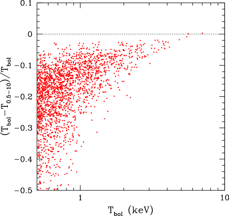
Figure 3: The fractional variation of the emission–weighted temperature, $T_{\rm ew}$, when using the bolometric and the [0.5–10] keV band emissivity.

While all this is true under the assumption of vanishing metallicity, including metals has the effect of biasing temperatures towards lower values (Mathiesen & Evrard 2001). The presence of metals increases the emissivity of relatively cold particles, thanks to the contribution of soft lines. Mathiesen & Evrard (2001) estimated this effect to lead to an underestimate of the temperature by about 20 per cent. Since our cooling function has been computed for zero metallicity, we do not to include this effect here. However, this emphasizes that a careful like-with-like comparison with observations is not always straightforward, and requires a careful treatment of physical processes when running simulations (in this case, the contribution of metal cooling), and of observational biases when analyzing them. The contribution from metal lines is expected to affect estimates of $T_{\rm ew}$ and, to a larger extent, of $L_{X}$ for systems with $T\raise-2.0pt\hbox{\hbox to0.0pt{\hbox{$\sim$}\hss}\raise 5.0pt\hbox{$<$}\ }2$ keV. However, these corrections become negligible at higher temperatures, where bremsstrahlung dominates the emissivity.

3.3 Luminosity profiles

X-ray surface brightness profiles represent a direct test bed to establish the existence (or lack) of self–similarity between clusters and groups. Ponman et al. (1999) actually presented a case against self–similarity: based on ROSAT-PSPC data, they pointed out that a continuous change of the mean surface–brightness profiles exists when going from poor groups to rich clusters. While it was found that this picture does not necessarily apply to hot ($T\raise-2.0pt\hbox{\hbox to0.0pt{\hbox{$\sim$}\hss}\raise 5.0pt\hbox{$>$}\ }3$ keV) systems (e.g., Neumann & Arnaud 1999), subsequent studies have indeed confirmed that groups in general show a shallower profile than rich clusters. This effect is usually quantified by fitting the observed profiles with standard $\beta$–models for the gas density (Cavaliere & Fusco–Femiano 1976),

$$\rho_{\rm gas}(r)\,=\,{\rho_{0}\over\left[1+(r/r_{c})^{2}\right]^{3\beta_{\rm fit}/2}}\,.$$ (3)

Observationally, $\beta_{\rm fit}$ appears to be an increasing function of temperature (e.g., Helsdon & Ponman 2000; Finoguenov et al. 2001, F01 hereafter; Sanderson et al. 2003).

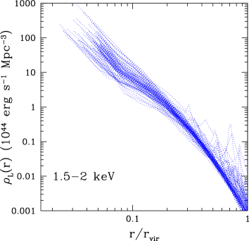
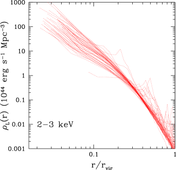
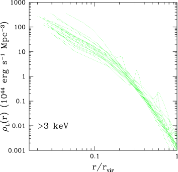
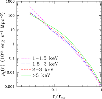
Figure 4: Profiles of luminosity density at different intervals of $T_{\rm ew}$. The upper and the lower left panels show all the profiles for structures within different temperature intervals. The lower right panel shows the average profiles computed within each range of $T_{\rm ew}$.

In Figure 4, we show the profiles of luminosity density, $\rho_{L}(r)$, for groups and clusters within different temperature intervals. We only compute profiles down to a radius which contains 100 SPH particles. This scale has been shown to be the smallest one where numerically converged results for the X-ray luminosity can be computed (Borgani et al. 2002) and, on average, it is about two times larger than $\epsilon_{\rm soft}=2.8\times\epsilon_{\rm Pl}$, i.e., the softening scale where gravitational force starts deviating from the $1/r^{2}$ law.

Quite remarkably, once the luminosity profiles are rescaled to the virial radius, $r_{\rm vir}$, they look very similar in the outer regions, $r\raise-2.0pt\hbox{\hbox to0.0pt{\hbox{$\sim$}\hss}\raise 5.0pt\hbox{$>$}\ }0.3r_{\rm vir}$, while the scatter significantly increases in the innermost regions. This result is in qualitative agreement with the findings by Neumann & Arnaud (1999). When looking at the average profiles (bottom right panel), it is seen that they all match when the virial radius is approached. However, down to about $0.1r_{\rm vir}$, colder systems tend to have a slightly shallower profile, which becomes steeper than that of hot systems at smaller radii.

The steepening of the gas density profile in the central regions of groups is the result of the cooling and star–formation process. Since cooling is relatively more efficient in smaller systems, as also witnessed by the increasing stellar fraction at low–$T$ (see Fig. 2), these systems tend to have stronger compressional heating of gas flowing toward central regions, as a consequence of the lack of pressure support. On the other hand, simulated clusters with $T>3$ keV do not exhibit any spike in emissivity associated with their central cooling regions.

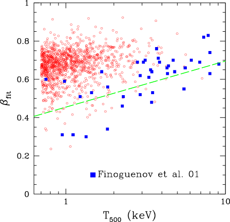
Figure 5: Comparison between the simulated (open circles) and observed (filled squares, from Finoguenov et al. 2001) values of the $\beta_{\rm fit}$–parameter obtained by fitting the gas density profiles to the $\beta$–model of Eq. (3). The dashed line is the best–fitting model to the data by Sanderson et al. (2003), $\beta_{\rm fit}=0.439\,T^{0.20}$.

In order to compare our profiles to observational data, we fitted our simulated gas–density profiles to the $\beta$–model of Eq. (3), and compared the result to the compilation of $\beta_{\rm fit}$ values by F01. Gas density profiles in simulated clusters are known to progressively steepen towards outer regions, thus implying that the resulting $\beta_{\rm fit}$ may depend on the range of scales where the fit is carried out. For this reason, the range of scales used for the fit should be chosen similar to the one that was used in the analysis of observational data. As for the outer radius, we choose to stop at $r_{500}$, which is close to the average outermost radius used in the analysis of F01, while we adopted $0.2\,r_{\rm vir}$ for the inner radius, which roughly corresponds to the radius at which the luminosity profiles change their slopes (see Fig. 4).

The result of this analysis is shown in Figure 5, where the $\beta_{\rm fit}$ values for simulated clusters are compared to the observational data points by F01 and to the best–fit relation by Sanderson et al. (2003). The simulation results are consistent with $\beta_{\rm fit}\simeq 0.7\pm 0.1$, with only a slight tendency for hotter systems to have larger values of $\beta_{\rm fit}$, a much weaker trend than inferred from observations. While the resulting $\beta_{\rm fit}$ values are consistent with the profiles of hot clusters, simulated groups tend to have steeper gas density profiles than observed. We verified that this result is robust against reasonable variations of the range of scales where the fit is realized. Reducing the inner radius to the smallest resolved scale does not produce any appreciable improvement in the comparison with data, neither it introduces any significant trend for a smaller $\beta_{\rm fit}$ at the scale of groups. On the other hand, increasing the outer radius to $r_{200}$ increases the resulting $\beta_{\rm fit}$ (as first pointed out by Navarro et al. 1995) and, therefore, makes the disagreement worse. This confirms that neither cooling nor our description of SN feedback are efficient enough to reduce the gas density at the center of poor clusters and groups to the observed level.

A still more faithful comparison with data would require treating simulated clusters exactly on the same footing as the real ones, by carefully choosing the same range of scales for sampling the luminosity profiles. Vikhlinin et al. (1999) pointed out that fitting profiles out to $\simeq r_{\rm vir}$ provides slightly larger values of $\beta_{\rm fit}$, by about 0.05, a trend that is also seen in simulations. However, such a small increase is not enough for interpreting the trend of $\beta_{\rm fit}$ with cluster temperature, as a result of poorer objects being sampled over smaller portions of their virial regions. Sanderson et al. (2003) have recently addressed this point by analysing two clusters for which ROSAT–PSPC data extends out to quite large radii. They found no significant evidence of steepening as the fitting region is enlarged, although this conclusion is based on only two fairly hot systems. The situation is likely to improve in coming years as more Chandra and XMM–Newton data will accumulate, allowing better sampling of the gas density in the outer regions of clusters and groups.

3.4 Temperature profiles

Observational data from spatially resolved spectroscopy with the ASCA (e.g., Markevitch et al. 1998), Beppo–SAX (De Grandi & Molendi 2002) and XMM–Newton (e.g., Pratt & Arnaud 2002) satellites show that temperature profiles decline at cluster–centric distances larger than about one quarter of the virial radius (see the data points in the left panel of Figure 7; cf. also Irwin & Bregman 2000). Furthermore, Beppo–SAX (De Grandi & Molendi 2002; Ettori et al. 2002a), Chandra (Ettori et al. 2002b; Allen, Schmidt & Fabian 2001; Johnstone et al. 2002) and XMM–Newton (Tamura et al. 2001) data show that temperature profiles smoothly decline towards the cluster center. In particular, Allen et al. (2001, A01 hereafter) analysed Chandra data for 6 fairly relaxed hot clusters, with $T\raise-2.0pt\hbox{\hbox to0.0pt{\hbox{$\sim$}\hss}\raise 5.0pt\hbox{$>$}\ }5.5$ keV. They found profiles which are quite similar once they are rescaled to $R_{2500}$ (the radius encompassing an average density $\bar{\rho}/\rho_{\rm crit}=2500$): an isothermal profile in the range $0.3\raise-2.0pt\hbox{\hbox to0.0pt{\hbox{$\sim$}\hss}\raise 5.0pt\hbox{$<$}\ }/R_{2500}\raise-2.0pt\hbox{\hbox to0.0pt{\hbox{$\sim$}\hss}\raise 5.0pt\hbox{$<$}\ }1$, with a smooth decline at smaller radii (dashed curve in the right panel of Fig. 7).

While a declining profile in the outer cluster regions is generally expected from hydrodynamical simulations (e.g., Evrard et al. 1996; Eke et al. 1998; Borgani et al. 2002; Loken et al. 2002; Rasia et al. 2003; Ascasibar et al. 2003), the presence of a nearly isothermal core with a central smooth temperature drop represents a significant challenge. In fact, including cooling and star formation in simulations has the effect of steepening the central temperature profile (e.g., Lewis et al. 2000; Muanwong et al. 2002; Valdarnini 2003), opposite to the observed decline of temperature. This is because cooling generates a lack of pressure support in central regions, which causes gas infall from outer regions, and this gas is heated by adiabatic compression as it streams towards the centre (e.g., Tornatore et al. 2003). A possible remedy of this disagreement may lie in extra heating of the ICM: placing the gas on a higher adiabat should reduce both the amount of cooling and the compressional heating. However, Tornatore et al. (2003) demonstrated that it is not easy to obtain this effect, even when a variety of heating prescriptions as in their study are explored.

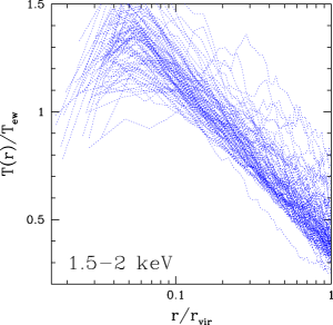
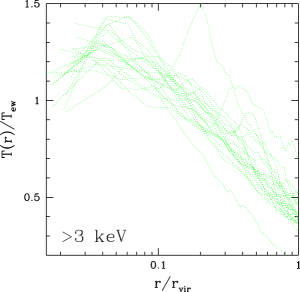
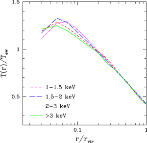
Figure 6: The temperature profiles for objects of different temperatures. The left and the central panels show individual profiles, while the right panel shows the average profiles for groups and clusters within different interval of $T_{\rm ew}$.

In Figure 6, we show the three–dimensional temperature profiles for our clusters and groups within different intervals of $T_{\rm ew}$. Although there is a considerable scatter among these profiles, they are all increasing with similar slopes down to $\simeq 0.05\,r_{\rm vir}$, with a temperature drop taking place only in the innermost regions. Individual profiles, rather than being smooth, are characterized by wiggles which are associated either with merging sub–groups that contain relatively cold gas, or with supersonic accretion which heats the gas across the shock fronts. These effects cause the complex temperature structures detected in real clusters (e.g., Mazzotta et al. 2002; Markevitch et al. 2003), and they are now routinely reproduced in high-resolution simulations (e.g., Bialek, Evrard & Mohr 2002; Motl et al. 2003; Tormen, Moscardini & Yoshida 2003).

In the right panel of Figure 6, we plot the average profiles for systems of different temperatures. Clusters and groups follow a nearly universal temperature–profile, with only a marginal tendency for hot systems to have shallower profiles at $r\raise-2.0pt\hbox{\hbox to0.0pt{\hbox{$\sim$}\hss}\raise 5.0pt\hbox{$<$}\ }0.2\,r_{\rm vir}$. In general, these profiles show neither evidence for an isothermal core, nor a central smooth decline down to about 1/2 of the virial temperature, as it is observed in many real clusters.

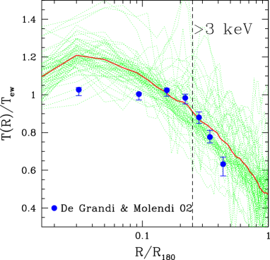
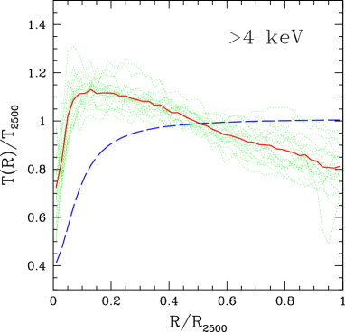
Figure 7: Comparison between simulated and observed projected temperature profiles. Left panel: comparison between simulated clusters with $T_{\rm ew}>3$ keV and the observational data points from the analysis of Beppo–SAX data for 17 clusters by De Grandi & Molendi (2002); projected radial scales are in units of $R_{180}$, i.e. the radius at which $\bar{\rho}/\rho_{\rm cr}=180$. Right panel: comparison between simulated clusters with $T_{\rm ew}>4$ keV and the best–fitting universal temperature profiles measured by Allen et al. (2001) from their analysis of Chandra data for a set of six relaxed clusters (dashed curve); projected radial scales are in units of $R_{2500}$. In both panels, dotted lines are the profiles for each single simulated cluster, while the heavy solid line is for the average profile. For reference, the vertical dashed line in the left panel indicates the average value of $R_{2500}$.

A more direct comparison with observations is given in Figure 7, where we compute projected profiles for the simulated clusters. For a proper comparison with the results by De Grandi & Molendi (2002), we select only clusters with $T>3$ keV, which is the range covered by their 17 clusters observed with Beppo–SAX. For each of the 23 simulated clusters with $T>3$ keV thus selected, we plot the profiles projected along three orthogonal directions. After projection, the average profile of the simulated clusters does still not show evidence for an isothermal core. They steadely increase toward the cluster center down to $R\raise-2.0pt\hbox{\hbox to0.0pt{\hbox{$\sim$}\hss}\raise 5.0pt\hbox{$>$}\ }0.04R_{180}$ (we define $R_{180}$ as the radius at which $\bar{\rho}/\rho_{\rm cr}=180$), while a temperature decrease is observed only in the innermost regions. It is worth noting that the slope of the simulated profile in the outer regions is similar to, although slightly shallower than, the observed one, thus in agreement with the “universal” temperature profile that Loken et al. (2002) obtained for simulations without cooling.

To further demonstrate the failure of the simulation to account for the observed central temperature profiles, we compare our results in the right panel of Fig. 7 to those obtained by A01 for a set of six fairly relaxed clusters with temperatures $T_{2500}$ in the range 5.5 to about 15 keV. Since in this range we have only one cluster, with $T\simeq 7$ keV, we also use our five clusters with $T>4$ keV for the comparison. This should not introduce any systematics, at least as long as hot clusters are self–similar, which is actually one of the claims made by A01. X–ray spectroscopy at high spatial resolution with Chandra opened the possibility to trace the temperature structure of such clusters down to unprecedented small scales, which are, however, easily accessible by our simulation. Again, the observed universal profile by A01 largely deviates from the simulated one. We point out that the profiles from the simulation show considerably more scatter than those of real clusters, but this is just due to the fact that we did not attempt to select relaxed clusters only. Nevertheless, we emphasize that in no case we find a cluster having an isothermal region followed by a smooth decline at $R\raise-2.0pt\hbox{\hbox to0.0pt{\hbox{$\sim$}\hss}\raise 5.0pt\hbox{$<$}\ }0.3\,R_{2500}$.

We argue that this discrepancy between simulated and observed temperature profiles is strong evidence for the current lack of self–consistent simulation models capable of explaining the thermal structure of the ICM in the regime where radiative cooling and feedback heating are highly important. We shall further discuss this point in Section 4.

3.5 The luminosity–temperature relation

Earlier on, it has been recognized that the $L_{X}$–$T$ relation of clusters provides evidence for a lack of self–similarity in the ICM properties (e.g., Evrard & Henry 1991; Kaiser 1991). Its shape at the cluster scale, $T\raise-2.0pt\hbox{\hbox to0.0pt{\hbox{$\sim$}\hss}\raise 5.0pt\hbox{$>$}\ }2$ keV, is well described by $L_{X}\propto T^{\alpha}$ with $\alpha\simeq 2.5$–3 (e.g., White et al. 1997; Xue & Wu 2000), with a possibly shallower slope that approaches the self–similar expectation of $\alpha=2$ for the very hot systems (Allen & Fabian 1998), and a considerably reduced scatter once cooling flow clusters are removed (Arnaud & Evrard 1999; Ettori et al. 2002a), or when the contribution from cooling regions is excised (e.g., Markevitch 1998). Furthermore, evidence has been found that groups with $T_{X}<2\,{\rm keV}$ have a significantly steeper slope of $\alpha\sim 5$ (e.g., Sanderson et al. 2003, and references therein), although this result is not confirmed by the analyses by Mulchaey & Zabludoff (1998) and Osmond & Ponman (2003).

In Fig. 8, we show a comparison between the observed and simulated $L_{X}$–$T$ relations for clusters and groups. Quite apparently, the simulation results reproduce the observations reasonably well on cluster scale. A log–log least–square fit to the relation

$$\log\left({L_{X}\over L_{X,0}}\right)\,=\,\alpha\,\log\left({T_{500}\over{\rm keV}}\right)$$ (4)

for clusters with $T>2$ keV gives $\alpha=2.5\pm 0.1$ and $L_{X,0}=(1.0\pm 0.3)\,10^{43}\,{\rm erg\,s^{-1}}$, with intrinsic scatter ${\Delta T\over T}=0.33$. Including colder systems in the fit, down to $T_{\rm ew}=0.7$ keV, confirms the visual impression that no significant change of slope takes place in the simulation at the scale of groups, thus consistent with the result found by Muanwong et al. (2002). While this is in contradiction with observational claims for a steepening on group scales (e.g., Ponman et al. 1996; Helsdon & Ponman 2000; Sanderson et al. 2003), it agrees with other analyses which indicate a unique slope from the cluster to the group scales (Mulchaey & Zabludoff 1998). Osmond & Ponman (2003) have recently analysed ROSAT–PSPC data for an extended set of galaxy groups and, although within a large scatter, found no evidence for a steepening of the $L_{X}$–$T$ relation.

From an observational point of view, determining the X–ray luminosity contributed by the diffuse medium in galaxy groups is not as straightforward as for richer clusters, mainly due to the uncertainties in removing the contribution from member galaxies, especially from the dominant ellipticals. For instance, if genuine emission from the diffuse intra–group medium is removed when excising galaxies, then the X–ray luminosity may be underestimated, thus leading to a steepening of the $L_{X}$–$T$ relation. This point was quite critical when considering pre–Chandra X–ray imaging, due to the limited spatial resolution. However, there is no doubt that, as Chandra data for a critical number of groups accumulates, it will become possible to settle the question of how much of the X–ray emission in central group regions has to be assigned to the diffuse medium.

Quite interestingly, the intrinsic scatter in the simulated $L_{X}$–$T$ relation is rather small, comparable to the 30 per cent value reported by Arnaud & Evrard (1999), even though we did not attempt to correct for the contribution of cooling regions. This is consistent with our finding from Fig. 4 where we do not detect significant spikes of emissivity associated with central cooling regions. In order to examine this further, we decided to apply to our clusters with $T_{X}>2\,{\rm keV}$ the procedure adopted by Markevitch et al. (1998) for excising the contribution from cooling regions. We first masked regions smaller than 50 $h^{-1}$ kpc and then multiplied the resulting $L_{X}$ by a factor 1.06 to account for the flux inside the masked regions, thereby assuming a $\beta$–model with $\beta_{\rm fit}=0.6$ and core radius of 125 $h^{-1}$ kpc. As a result, we find that this procedure affects the $L_{X}$ values only marginally, thus having only a negligible effect on the scatter of the $L_{X}$–$T$ relation.

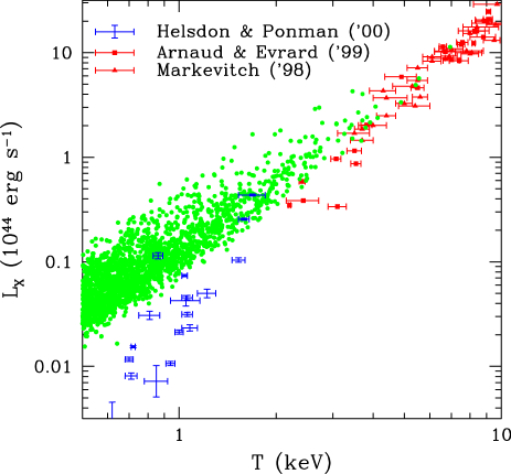
Figure 8: Comparison between the observed and the simulated relation between bolometric luminosity, $L_{X}$, and emission–weighted temperature, $T_{\rm ew}$. The latter has been computed weighting the contribution from each gas particle according to its emissivity in the [0.5-10] keV energy band.

3.6 The mass–temperature relation

It is a well known problem of hydrodynamical simulations of cluster formation with gravitational heating only that they predict a normalization of the relation between total self–gravitating mass and ICM temperature which is about 40 per cent higher than observed (e.g., Evrard et al. 1996). This means that, for a fixed mass, simulated clusters tend to be colder than observed (e.g., Horner, Mushotzky & Scharf 1999; Nevalainen, Markevitch & Forman 2000; F01; A01; Ettori et al. 2002a; Sanderson et al. 2003). On the scale of groups, the slope of the mass–temperature relation is possibly also steeper than the $M\propto T^{3/2}$ predicted by hydrostatic equilibrium.

A possible interpretation for this discrepancy is that non–gravitational heating increases the ICM temperature at a fixed mass, thus lowering the $M$–$T$ amplitude. However, hydrodynamical simulations that include non–gravitational heating have demonstrated that this leaves only a negligible imprint in the $M$–$T$ relation: after being preheated, the ICM settles back into hydrostatic equilibrium, with its temperature being determined by the DM–dominated gravitational potential well (Borgani et al. 2002). Another possible explanation relies on the effect of radiative cooling (e.g., Thomas et al. 2001; Voit et al. 2002). Although this may appear counterintuitive, radiative cooling may actually increase the ICM temperature, because it eliminates central pressure support, thus causing gas from outer regions to flow in and be heated by adiabatic compression. Although simulations do show such an effect to some extent, it is not clear whether cooling alone is able to reconcile the simulated and observed mass–temperature relations (e.g., Muanwong et al. 2002; Tornatore et al. 2003). Furthermore, for $T_{\rm ew}$ to increase by the required amount, one is forced to increase the ICM temperature in central regions, thus steepening the temperature profiles. As already discussed this is not a welcome feature.

The left panel of Figure 9 actually demonstrates that cooling in our simulation is not effective in reducing the $M$–$T$ normalization to the observed level. In this panel, our results are compared to those by F01. Making a log–log least square fitting to the relation

$$\log\left({M_{500}\over M_{0}}\right)\,=\,\alpha\,\log\left({T_{500}\over{\rm keV}}\right),$$ (5)

we obtain $\alpha=1.59\pm 0.05$ and $M_{0}=(2.5\pm 0.1)\,10^{13}h^{-1}M_{\odot}$. Therefore, the normalization of our relation at 1 keV turns out to be higher by about 20 per cent than that found by F01, while it is lower by about 20 per cent with respect to that found by Evrard et al. (1996) from simulations not including radiative cooling. The intrinsic scatter around the best–fitting relation is $\Delta M/M=0.16$. Since simulation data have no measurement error, this has to be interpreted as the intrinsic scatter which originates from cluster dynamics.

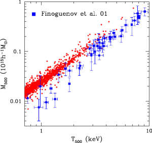
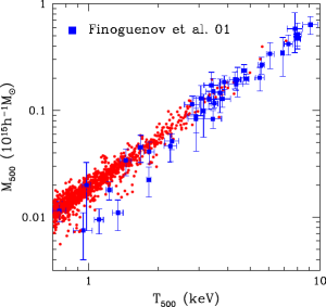
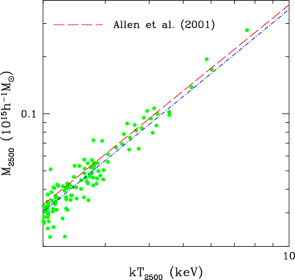
Figure 9: Comparison between the observed and the simulated $M$–$T$ relation. Left and central panels refer to the relation at $\bar{\rho}/\rho_{c}=500$. In the left panel we compare the results from Finoguenov et al. (2001, F01) to the true total masses of simulated clusters. In the central panel, cluster masses are estimated by reproducing the procedure followed by F01 (see text): the equation of hydrostatic equilibrium is applied after fitting the gas density profile to a $\beta$–model and assuming a polytropic equation of state. In the right panel the simulation results at $\bar{\rho}/\rho_{c}=2500$ (points) are compared to the relation found by Allen et al. (2001, A01) from Chandra for hot relaxed clusters (dashed line); the dot–dashed line is our best–fit to the clusters with $T_{2500}>2$ keV; we note that in this case $T_{2500}$ should be interpreted as a mass–weighted temperature (see text).

A critical issue in this comparison concerns the different procedures used for estimating masses in simulations and in observations. For instance, Markevitch et al. (1998), Nevalainen et al. (2000) and F01 estimate masses by applying the equation of hydrostatic equilibrium, assuming a $\beta$–model for the gas density profile and a polytropic equation of state of the form $T\propto\rho_{\rm gas}^{\gamma-1}$, where $\gamma$ is an effective polytropic index. Under these assumptions, hydrostatic equilibrium provides the total self–gravitating mass within the radius $r$ as

$$M(<r)\,=\,1.11\times 10^{14}\beta_{\rm fit}\gamma{T(r)\over{\rm keV}}{r\over\,h^{-1}{\rm Mpc}}{x^{2}\over 1+x^{2}}\,,$$ (6)

where $T(r)$ is the temperature at the radius $r$, $x=r/r_{c}$ is a scaled radial coordinate in units of the core radius $r_{c}$ of the gas density profile, and we assumed $\mu=0.6$ for the mean molecular weight. Based on hydrodynamical cluster simulations, Bartelmann & Steinmetz (1996) questioned this procedure and suggested that the limited range of scales where the $\beta$–model provides a good fit may bias cluster mass estimates low by as much as 40 per cent (see also Muanwong et al. 2002).

In order to verify this, we estimate cluster masses by applying Eq. (6). For each cluster, we compute $\beta_{\rm fit}$ by fitting the gas density profile to the $\beta$–model (see Fig. 5), and $\gamma$ by fitting temperature and gas–density profiles to the polytropic equation of state over the same range of radii. The resulting values of $\gamma$ are compared in Figure 10 to those reported by F01. Despite the fairly large observational uncertainties, simulation results generally agree with observations, with $\gamma\simeq 1.2$ and no dependence on cluster temperature. As for the core radius, both theoretical arguments (e.g., Komatsu & Seljak 2001) and observational data (e.g., F01) indicate that it is generally of the order of one–tenth of $r_{500}$ so that the correction term in Eq. (6) for the presence of a finite core is negligible.

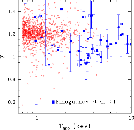
Figure 10: Comparison between the simulated (open circles) and the observed (filled squares, from Finoguenov et al. 2001) values of the effective polytropic index $\gamma$.

As shown in the central panel of Fig. 9, the effect of using Eq. (6) as a mass estimator is that of lowering the normalization of the $M$–$T$ relation and to bring it into better agreement with observations. While the slope and the intrinsic scatter are left essentially unchanged, with $\alpha=1.57\pm 0.02$ and $\Delta M/M\simeq 0.17$, the normalization is decreased to $M_{0}=(1.9\pm 0.1)\,10^{13}h^{-1}M_{\odot}$. The main reason for the biasing towards low mass estimates lies in the limited range of scales used to fit the $\beta_{\rm fit}$ parameter. In fact, we have verified that, if we extend the fit out to the virial radius, the average value of $\beta_{\rm fit}$ increases by about 15 per cent and, therefore, so does the mass estimate. This result indicates that possible biases in the observational mass estimates, related to the assumptions of $\beta$–model profile and hydrostatic equilibrium (see also the discussion by Rasia et al. 2003, and Ascasibar et al. 2003), may be at the origin of the difference between our simulated $M$–$T$ relation and the observed one.

With the availability of data of better quality from Chandra and XMM–Newton, one can avoid some of the assumptions that enter the derivation of Eq. (6). Based on Chandra observations, A01 realized high–resolution imaging and spatially resolved spectroscopy for six relaxed clusters with $T\raise-2.0pt\hbox{\hbox to0.0pt{\hbox{$\sim$}\hss}\raise 5.0pt\hbox{$>$}\ }5.5$ keV. Instead of assuming a $\beta$–model and a polytropic equation of state, they applied a deprojection technique to temperature and surface brightness profiles (e.g., White et al. 1997) in order to reconstruct gas mass and total mass profiles, assuming that the latter can be parametrized with a NFW model (Navarro, Frenk & White 1997). As such, the $M$–$T$ relation obtained from their analysis can be directly compared to the simulation result based on the “true” cluster masses. Given the relatively small field-of-view of the ACIS-S Chandra detector, they however had to restrict their analysis to $R_{2500}$. The resulting best–fitting $M_{2500}$–$T_{2500}$ relation is plotted as a dashed line in the right panel of Fig. 9 and compared to the results of our simulation. Thanks to the possibility of resolving temperature profiles, the values of $T_{2500}$ provided by A01 are computed by mass–weighting the temperature determinations in different radial bins. In order to reproduce the procedure followed by A01, we compute $T_{2500}$ in simulated clusters by mass–weighting the corresponding temperature profiles. After fitting our results to the power–law scaling of the $M_{2500}$–$T_{2500}$ relation for the clusters with $T_{2500}>2$ keV, we obtain $\alpha=1.55\pm 0.05$ and $M_{0}=(1.0\pm 0.2)\,10^{13}h^{-1}M_{\odot}$.

It is quite remarkable that the simulation results now agree with observations on the $M$–$T$ relation. Admittedly, given the small number of hot clusters in our simulation, this comparison is based on assuming that the best–fit relation by A01 can be extrapolated to colder systems. Still, this result suggests that observed and simulated $M$–$T$ relations agree with each other when high–quality observational data are used which accurately resolves the surface–brightness profile and the temperature structure of clusters.

According to the above discussion, comparing the observed and the simulated $M$–$T$ relation requires understanding how mass is estimated from data. At the same time, it is also important to understand how measured temperatures compare to the temperature inferred from simulations. As we discussed in Section 3.2, including the effect of metal lines could bias low the observed temperature, thus affecting the $M$–$T$ relation (e.g., Mathiesen & Evrard 2001). Accounting for these effect requires to self–consistently trace the pattern of metal enrichment and to reproduce in detail the observational setup. This will become mandatory as the level of precision at which the X–ray properties of real and virtual clusters increases.

One of the most important applications of the calibration of the $M$–$T$ relation and of its intrinsic scatter is to obtain cosmological constraints from the cluster X–ray luminosity function (XLF) and temperature function (XTF). Of particular interest is the normalization of the power spectrum in terms of $\sigma_{8}$. The lower the normalization of the $M$–$T$ relation, the smaller the mass of collapsed halos to be identified with clusters of a given temperature, and consequently, the lower the normalization of the power spectrum required for a given cosmological model to fit the observed XTF (e.g., Ikebe et al. 2002; Seljak 2002; Pierpaoli et al. 2003, and references therein). Huterer & White (2002) have shown that, to a good approximation, the values of $\Omega_{m}$ and $\sigma_{8}$ scale with the normalization $M_{0}$ of the mass–temperature relation as $\Omega_{m}^{0.6}\sigma_{8}\propto M_{0}^{0.53}$. If we take the result of our analysis that the observed $M_{0}$ may be biased low by about 25 per cent at face value, we would then expect that the infered $\sigma_{8}$ should be biased low by almost 15 per cent. Furthermore, the value of the intrinsic scatter in the $M$–$T$ relation also affects the determination of $\sigma_{8}$ from the cluster XLF and XTF (e.g., Borgani et al. 2001b; Pierpaoli et al. 2003). In the presence of a significant scatter, the model–predicted distribution functions are given by the convolution of the cosmological mass function with a Gaussian function with width equal to this scatter. Therefore, the larger the scatter, the lower the power spectrum normalization required to fit the observed XLF or XTF.

Thanks to the good statistics offered by our simulation, a reliable calibration of the scatter expected in the $M$–$T$ relation can be obtained. We suggest that this calibration should be used for the determination of cosmological parameters from the XTF and XLF. This shows the importance of a precise calibration of the relations between theory–predicted mass and X–ray observed quantities (e.g. Rosati, Borgani & Norman 2002, and references therein), and highlights the important role that large cosmological simulations can play in understanding the systematics involved (e.g., Viana et al. 2003).

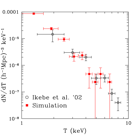
Figure 11: Comparison between the simulated XTF at $z=0$ (filled squares) and the local XTF measured for the sample by Ikebe et al. (2002), and adapted for the simulated cosmological model (open circles; Ikebe, private communication). Error bars in the simulated XTF correspond to Poissonian uncertainties within each temperature bin.

In order to verify whether, with the chosen value of $\sigma_{8}=0.8$, the simulation produces the correct cluster number density, we compare in Figure 11 the XTF from our clusters to that reported by Ikebe et al. (2002), adapted to our cosmological model (Ikebe, private communication). Although our limited box size makes the comparison difficult for $T>6\,{\rm keV}$, we note that our simulated XTF agrees with the observed one remarkably well over the common temperature range. Since there are no adjustable parameters in the estimate of our XTF, this indicates that $\sigma_{8}\simeq 0.8$ (for a flat model with $\Omega_{m}=0.3$) is in fact required to match the observed number density of nearby clusters.

3.7 The $M_{\rm gas}$–$T$ relation

The mass of diffuse gas is a quite useful diagnostic for the physical status of the ICM, since it is free from several of the uncertainties which affect the estimate of the total self–gravitating mass. Under the assumption that gas follows dark matter, we expect that the gas fraction in clusters, $f_{\rm gas}$ is independent of cluster mass and, therefore, $M_{\rm gas}\propto T^{3/2}$. Measurements of the gas mass from X–ray observations have shown that the observed relation between gas mass and temperature can indeed be represented by a power law, $M_{\rm gas}\propto T^{\alpha}$, but with a slope which is generally steeper than this self–similar expectation. For instance, Vikhlinin et al. (1999) fitted gas density profiles out to $R_{200}$ and found $\alpha=1.71\pm 0.13$. Other estimates of the $M_{\rm gas}$–$T$ scaling at higher overdensity find steeper slopes. Mohr et al. (1999) analysed a set of clusters with $T\raise-2.0pt\hbox{\hbox to0.0pt{\hbox{$\sim$}\hss}\raise 5.0pt\hbox{$>$}\ }2$ keV at $\bar{\rho}/\rho_{cr}=500$ and found $\alpha=1.98\pm 0.18$, while Ettori et al. (2002a) found $\alpha=1.91\pm 0.29$ at $\bar{\rho}/\rho_{cr}=2500$ for a sample of $T>3$ keV clusters. These results show that colder systems tend to be less gas-rich, an effect which is more pronunced at higher overdensity. These trends are naturally expected in scenarios where self–similarity is broken by extra heating (e.g., Bialek et al. 2001), which prevents gas from reaching high density in central regions. Cooling can in principle also account for the observed $M_{\rm gas}$–$T$ relation, provided its efficiency is significantly higher in groups than in rich clusters.

In order to compare results from our simulation with observations, we make a log–log least–square fitting to the expression

$$\log\left({M_{\rm gas}\over M_{0}}\right)\,=\,\alpha\,\log\left({T\over{\rm keV}}\right)\,.$$ (7)

We find $\alpha=1.80\pm 0.08$ and $M_{0}=(1.8\pm 0.2)\,10^{12}h^{-1}M_{\odot}$ when fitted at $R_{500}$ for clusters with $T_{500}>2$ keV. As shown in Figure 12, the simulated relation tends to be shallower than the observed one, thus further indicating that the feedback energy provided by our modelling of SN explosions is not strong enough to break self–similarity as strongly as observed. Note however that if a stronger heating was realized, the effect would be that of suppressing $M_{\rm gas}$ more strongly in low–mass systems, thereby reducing the overall normalization below the observed level. The offset in the normalization is likely to be due to two main reasons. First, since cooling in the simulation is too efficient, too large a fraction of gas is removed from the X–ray emitting phase. Therefore, reducing the cold phase to the observed level would imply a compensating increase of $M_{\rm gas}$ by about 10 per cent. Second, our run is based on assuming $\Omega_{\rm bar}=0.04$ for the baryon density parameter. If the 20 per-cent larger value indicated by WMAP data were used instead, this would have led to a corresponding increase of $M_{\rm gas}$ of similar size.

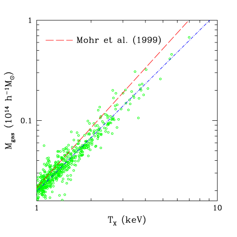
Figure 12: Comparison between the simulated (open circles) and observed $M_{\rm gas}$–$T$ relation at overdensity $\bar{\rho}/\rho_{cr}=500$. The dashed line is the best–fitting model by Mohr et al. (1999) to their observational data points, $M_{\rm gas}=2.1(T_{\rm ew}/{\rm keV})^{1.98}10^{12}h^{-1}M_{\odot}$, while the dot-dashed line is the best–fitting relation to the results of the simulation $M_{\rm gas}=2.0(T_{\rm ew}/{\rm keV})^{1.75}10^{12}h^{-1}M_{\odot}$.

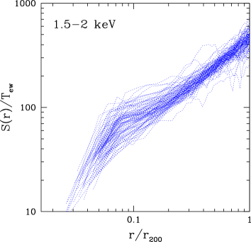
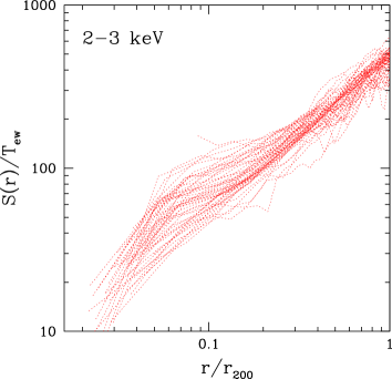
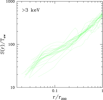
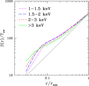
Figure 13: Profiles of reduced entropy, $S/T$, at different intervals of $T_{\rm ew}$. The upper and the lower left panels show the profiles for all the structures within each temperature interval. The lower right panel shows the average profiles computed within each range of $T_{\rm ew}$. In this panel the dotted line shows the scaling $S\propto r^{1.1}$, which is expected if entropy is generated by self–similar accretion shocks (Tozzi & Norman 2001).

3.8 The entropy of the ICM

Gas entropy is currently receiving considerable attention as a diagnostic tool for tracing the past dynamical and thermal history of the ICM (e.g., Bower 1997; Ponman et al. 1999; Tozzi & Norman 2001; Balogh et al. 2001; Borgani et al. 2001; Voit et al. 2002; Babul et al. 2002). In X–ray studies of galaxy clusters, the ‘entropy’ is commonly defined as

$$S\,=\,{T\over n_{e}^{2/3}}\,.$$ (8)

With this definition, $S$ is proportional to the adiabats of an ideal monoatomic gas, and is expressed in units of ${\rm keV\,cm}^{2}$. The relation of $S$ to the thermodynamic definition of entropy, $s$, is given by $s=c_{V}\log{S}+{\rm const}$, where $c_{V}$ is the specific heat capacity at constant volume.

As long as the gas adiabat is not altered by some non–gravitational heating source, one can derive the expected scaling between entropy and temperature at redshift $z$ in the form $S\propto T^{2}/(E_{z}^{2}\Delta_{c})^{2/3}$, where $E_{z}=[(1+z)^{3}\Omega_{m}+1-\Omega_{m}]^{1/2}$ describes the evolution of the Hubble constant and $\Delta_{c}$ is the overdensity, in units of the critical density, at which the entropy is measured. This implies that, once $\Delta_{c}$ is fixed, entropy has a linear dependence on gas temperature. In fact, when going from rich clusters to poor groups, we probe gas that has been accreted at higher redshift, when it was harder to generate accretion shocks and, therefore, to increase the gas entropy.

For this reason, the entropy excess measured in the central regions of poor clusters and groups (e.g., Ponman et al. 1999; Lloyd–Davies et al. 2000; Finoguenov et al. 2002) is considered to provide direct evidence that some non–gravitational process must have modified the gas adiabat. For instance, if some process establishes a pre–collapse entropy floor, we expect to measure the level of this floor at the center of poor clusters and groups, while the scaling $S\propto T$ should be recovered for hot systems, whose entropy creation has been dominated by gravitational shocks (e.g., Tozzi & Norman 2001). However, this scenario is now questioned by the detection of the so–called “entropy ramp” in central cluster regions (Ponman et al. 2003; see the data points plotted in Figure 14): instead of following the $S\propto T$ scaling for hot systems with a flattening to some floor for cold systems, entropy is shown to gradually deviate from the self–simular scaling, with a temperature dependence close to $S\propto T^{2/3}$. Predictions of the standard pre–heating scenario are also at variance with the results by Mushotzky et al. (2003) from XMM–Newton observations of two groups, which do no show any flattening of the entropy profiles in central regions.

These results therefore call for alternative scenarios for gas heating (e.g., Dos Santos & Doré 2002), or for a significant effect of radiative cooling. Counterintuitively, cooling has the effect of providing an increase of the entropy of the diffuse hot gas as a result of selective removal of low–entropy gas from the hot phase (e.g., Voit & Bryan 2001; Voit et al. 2002; Wu & Xue 2002). However, while numerical simulations have shown that cooling and star formation do indeed increase entropy in central cluster regions, they are not able to account for the large excess observed on the scale of groups (Finoguenov et al. 2003; Tornatore et al. 2003). Since these numerical results were based on simulations of a small number of halos, they were, however, suspicious of not being representative for the whole population of galaxy systems. This limitation is overcome by the fairly large set of clusters and groups available from our simulation.

In Figure 13, we show the profiles of the “reduced” entropy, $S/T$. Note that these profiles should coincide if clusters and groups are self–similar. Radii are given in units of $r_{200}$ so as to make our profiles directly comparable to those recently published by Ponman et al. (2003). At large radii the profiles approach the scaling $S(r)\propto r^{1.1}$, which is predicted in the shock–dominated regime of entropy production by models based on spherical gas accretion within a NFW dark matter halo (Tozzi & Norman 2001; see the dotted curve in the lower right panel). This demonstrates that gravity dominates the ICM thermodynamics in the outer regions of clusters. Quite interestingly, this also indicates that, although accretion is anisotropic in cosmological environments where subgroups and gas primarily flow along filaments onto the cluster (e.g. Tormen 1997), spherical accretion still provides an adequate average description.

Looking at the average profiles (lower right panel) it is then remarkable that they all fall on top of each other, almost independent of the temperature of the system. Although this is quite expected, as long as non–gravitational effects are negligible, it conflicts with the recent results by Ponman et al. (2003). These authors computed entropy profiles from ROSAT–PSPC and ASCA data for clusters and groups in the temperature range 0.3–17 keV. Although the profiles were found to be parallel to each other in the outer regions, and close to the $r^{1.1}$ scaling, colder systems turned out to have a relatively higher entropy. With an independent analysis, Pratt & Arnaud (2003) used XMM–Newton data for a cluster and a group, with well resolved temperature profiles. They consistently found the profiles of reduced entropy to be quite parallel to each other, with the group having a relatively higher entropy, although intrinsic scatter (see Fig. 13) may limit the significance of a result based only on two profiles.

Models based on an entropy floor or on cooling can account for the lack of self–similarity in central cluster regions, while they predict that all the systems follow self–similarity in regions close to the last–shock radius. Possible explanations for this global violation of self–similarity have been proposed by Ponman et al. (2003) and Voit et al. (2003), and are based on a differential entropy amplification by shocks in the presence of pre–heating. Smaller mass systems are expected to accrete from lower–density filaments. Therefore, pre–heating should be more efficient in evaporating condensations (Ponman et al.) and/or in suppressing gas density (Voit et al.) within the filaments accreting into groups, compared with those accreting into clusters. In turn, this would make shocks stronger and, therefore, entropy generation more efficient at the outskirts of colder systems. The fact that this is not detected in our clusters may imply that any pre–heating associated with SN energy feedback in our simulation is too week to have a sizeable effect.

The entropy level at $r\simeq 0.1\,r_{200}$ is a factor $\sim 2$ larger than what is expected from the extrapolation of the $r^{1.1}$ scaling. At smaller radii, the entropy profiles tend to steepen, which indicates the presence of a population of gas particles which start feeling the effect of cooling, while still belonging to the hot phase. This feature is more pronunced for smaller systems, whose relatively higher central density makes cooling more efficient (as also confirmed by their larger star fraction; see Fig.2). Still, at $r\simeq 0.1r_{200}$ there are no significant differences in the values of the reduced entropy. This is actually confirmed by Figure 14, where we compare the reduced entropy found for simulated clusters at $0.1\,r_{200}$ to the “entropy ramp” measured by Ponman et al. (2003). While our simulation confirms the existence of an entropy excess, its magnitude does not depend sensitively on temperature, in contrast to the observed gradual departure of entropy from the expectation of self–similar scaling (dashed line) when colder systems are considered.

This result corroborates the finding that the adopted recipe for supernova feedback from stellar populations, which includes comparatively weak galactic winds, is not strong enough to increase the gas adiabat in central cluster regions. At the same time, radiative cooling is not able by itself to break the self–similarity of the ICM entropy structure as strongly as observed. Muanwong et al. (2002) found a better agreement of simulations with the observational data by Ponman et al. (1999) with respect to the entropy level in the central region of groups. Besides the difference in the data set they are comparing to, the reason for this could also be due to the fact that their simulation assumed a global gas metallicity of $0.3\,Z_{\odot}$ at $z=0$ in the computation of the cooling function (although metal production was not treated in their code). A non–vanishing metallicity increases the cooling function and, therefore, increases the entropy level for gas removal from the hot phase (e.g., Voit & Bryan 2001).

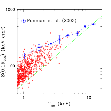
Figure 14: The relation between gas entropy computed at $0.1\,r_{\rm vir}$ and $T_{\rm ew}$. Data points are taken from Ponman et al. (2003). The dashed line shows for reference the self–similar scaling $S\propto T$, normalized to the hottest cluster found in the simulation.

4 Discussion and conclusions

We have presented results on the X–ray properties of groups and clusters of galaxies, extracted from a large hydrodynamical simulation within a cosmological box of $192\,h^{-1}{\rm Mpc}$ on a side. The simulation includes radiative gas cooling, heating from a uniform UV background, a description of star formation within a multi–phase interstellar medium and a phenomenological treatment of galactic winds, powered by supernova (SN) energy release. The quite high number of gas and DM particles used, $2\times 480^{3}$, and the force resolution of 7.5 $h^{-1}$kpc provide high enough mass and force resolution for an accurate description of the X–ray properties of galaxy systems down to a virial temperature of about 0.5 keV. The results of this simulation have been thoroughly compared to observational results on the X–ray properties of clusters. Rather than focusing on quantities that show good agreement between simulation and observations, this comparison was made in the spirit of better understanding how our current description of the physics of the ICM needs to be improved.

Our main results can be summarized as follows:

• The scaling relations of X–ray luminosity and gas mass with cluster temperature deviate from the predictions of self–similar scaling. However, in some cases these deviations are not as large as needed to agree with observations. For instance, the simulated $L_{X}$–$T$ relation provides a good fit to data at $T\raise-2.0pt\hbox{\hbox to0.0pt{\hbox{$\sim$}\hss}\raise 5.0pt\hbox{$>$}\ }2$ keV, while it does not produce any steepening at the scale of groups (e.g., Lloyd–Davies & Ponman 2000; cf. also Mulchaey & Zabludoff 1998). A recent analysis by Osmond & Ponman (2003) actually demonstrates that the present quality of data is not good enough to allow a precise determination of the $L_{X}$–$T$ scaling for galaxy groups. Furthermore, the $M_{\rm gas}$–$T$ relation is shallower than observed (e.g., Mohr et al. 1999; Ettori et al. 2002a).

• Consistently, the gas density profiles are steeper than observed, especially for groups. Fitting the profiles to a $\beta$–model gives $\beta_{\rm fit}$ in the range 0.6–0.8, with no appreciable dependence on temperature.

• The simulated $M$–$T$ relation is about 20 per cent higher than that measured from observations under the assumptions of a $\beta$–model in hydrostatic equilibrium with a polytropic equation of state (e.g., Horner et al. 1999; Nevalainen et al. 2000; Finoguenov et al. 2001). If masses of simulated clusters are estimated with this same procedure, they are found to be biased low by just the amount required to recover agreement with the observed $M$–$T$ relation. Quite interestingly, a good agreement is in fact found by comparing simulation results to the $M_{2500}$–$T_{2500}$ relation based on the Chandra data by Allen et al. (2001), which does not rely on the assumption of a specific gas density profile. This suggests that the problem of the $M$–$T$ normalization may be solved by a better data treatment.

• The X–ray temperature function (XTF) from the simulation agrees quite nicely with the most recent observational determinations (e.g., Ikebe et al. 2002; Ikebe, private communication). This indicates that the chosen power–spectrum normalization, $\sigma_{8}=0.8$, for $\Omega_{m}=0.3$ is consistent with the measured number density of galaxy clusters.

• Temperature profiles from the simulation are discrepant with respect to observations. While their shape in the outer regions, at $R\raise-2.0pt\hbox{\hbox to0.0pt{\hbox{$\sim$}\hss}\raise 5.0pt\hbox{$>$}\ }0.3R_{180}$, is similar to the observed one, simulation profiles are steadily increasing towards the centers, with no evidence for an isothermal regime (e.g., De Grandi & Molendi 2002) followed by a smooth decline at $R\raise-2.0pt\hbox{\hbox to0.0pt{\hbox{$\sim$}\hss}\raise 5.0pt\hbox{$<$}\ }0.3\,R_{2500}$ (e.g., Allen et al. 2001).

• The entropy properties of simulated clusters are also quite different from observational results. In the outer regions, the entropy profiles from the simulation are remarkably self–similar, while observations show evidence for excess entropy at the scale of groups (Ponman et al. 2003). In the inner regions, we detect a significant excess entropy whose amount is almost independent of the cluster temperature. Although the resulting $S$–$T$ relation therefore deviates from the self–similar expectation, it is anyway steeper than observed (Ponman et al. 2003).

• The fraction of baryons which cool and turn into stars within the virial regions of clusters is $f_{*}\simeq 20$ per cent, with a slight tendency to be higher for colder systems. This value is substantially smaller than the one found in simulations that do not include efficient feedback mechanisms, but it is still higher than observed by about a factor of two (e.g., Balogh et al. 2001; Lin et al. 2003). This demonstrates that the choice of SN feedback included in the simulation is not efficient enough to prevent overcooling. We note that in the simulations of Springel & Hernquist (2003b) lower stellar fractions were obtained, but these authors adopted galactic winds that were twice as energetic as the ones included here.

In general, these results show that the physical processes included in our simulation are able to account for the basic global properties of clusters, such as the scaling relations between mass, temperature and luminosity. At the same time, we find indications suggesting that a more efficient way of providing non–gravitational heating from feedback energy compared to what is implemented in the simulation is required: this ‘extra heating’ should not only reduce the amount of gas that cools, but also needs to ‘soften’ the gas density profiles of poor clusters and groups by increasing the entropy of the relevant gas. We also remind that the present simulation has been realized using a zero–metallicity cooling function. Although the effect of metal–line cooling is expected to marginally affect the overall cosmic star formation (e.g., Hernquist & Springel 2003), it is known to increase quite significantly the X–ray emissivity of gas at $T\raise-2.0pt\hbox{\hbox to0.0pt{\hbox{$\sim$}\hss}\raise 5.0pt\hbox{$<$}\ }2$ keV, as well as the efficiency in the removal of low–entropy gas from the hot phase (e.g., Voit et al. 2002).

We think that it is unlikely that the problems of the present simulation are caused by numerical limitations. The model for star formation and galactic winds triggered by SN-II feedback, as implemented in our simulation (Springel & Hernquist 2003a), has been demonstrated to have well-behaved numerical properties, and it produces a realistic and numerically convergent cosmic star–formation history (Springel & Hernquist 2003b) that can be accurately understood by analytic reasoning (Hernquist & Springel 2003). However, we note that here we adopted a less extreme wind model than Springel & Hernquist (2003b), with only half of the available SN-II powering the wind, not nearly all of it, as they assumed. If we had also adopted such stronger winds, the residual overcooling in our clusters would have been reduced.

This therefore indicates that additional feedback processes may be at work in the highly overdense environments of clusters and groups of galaxies, and that perhaps additional sources of energy beyond SN–II are involved. Based on semi–analytical modelling of galaxy formation, Menci & Cavaliere (2000) and Bower et al. (2001) argued that the feedback energy available from SN-II should actually be enough to heat the ICM to the desired level, the problem however is that this requires a very high, possibly unrealistic, efficiency for the thermalization of this energy. Of course, given a fixed energy budget available for heating, one can invoke ‘optimal’ ways of releasing it to the ICM to maximize its impact. For instance, one can postulate that energy feedback targets just those particles which are about to undergo cooling (e.g., Kay et al. 2003) or which have long enough cooling time (e.g., Marri & White 2003). Although such ad-hoc schemes are often explored in feedback recipes, one would prefer if they could be shown to arise as a natural consequence of a physically self–consistent model.

Other sources of energy appear therefore as increasingly attractive possibilities, for example SN-Ia. The energetics of SN-Ia is usually considered to be subdominant, otherwise they would produce too much Iron and overpollute the ICM (e.g., Renzini 1997, 2003; Pipino et al. 2002). On the other hand, because the progenitors of SN-Ia have a much longer life–time than those of SN-II, the corresponding energy is released more gradually into a medium which is already heated by the shorter–lived SN-II. This heated gas has hence already a longer cooling time, making SN-Ia potentially a much more efficient heating source than SN-II. However, a proper implementation in simulations requires that the assumption of instantaneous recycling is dropped (e.g., Lia, Portinari & Carraro 2002; Valdarnini 2003; Kay et al. 2003; Kawata & Gibson 2003; Tornatore et al. 2003, in preparation).

A further source of energy feedback, which is not included in our simulation, is represented by AGN. The energy output of AGN can be extremely large, of the order $2\times 10^{62}(M_{\rm BH}/10^{9}M_{\odot})$ erg, where $M_{\rm BH}$ is mass of the central supermassive black–hole. Theoretical calculations show that a fractional coupling of the energy released by the AGN with the surrounding ICM at the level of $f\approx 0.01$ would be sufficent to account for the $L_{X}$–$T$ relations of groups (Cavaliere et al. 2002). While a number of hydrodynamical cosmological codes now include a treatment for star formation and SN feedback, none of them includes yet a self–consistent treatment of energy release from AGN. As a first approximation to their effect, the corresponding feedback energy could simply be added to the energy budget provided by SN, which should be adequate as long as the nuclear activity follows the star formation within the hosting galaxies (e.g., Franceschini et al. 1999). However, dynamically consistent models of AGN within cosmological simulations of structure formation are clearly needed to understand their effects in detail.

Perhaps the most puzzling discrepancy with observations concerns the temperature profiles. Cooling causes a lack of pressure support in the cluster center, causing gas to flow in from outer regions, being heated by adiabatic compression (e.g., Tornatore et al. 2003). As a result, the temperature actually increases in cooling regions, causing steeply increasing temperature profiles. This picture is quite discrepant compared to the standard cooling-flow model, where a population of gas particles at very low temperature should be detected (see Fabian 1994, for a review). Even more importantly, it also conflicts with the observational picture emerging from Chandra and XMM–Newton observations: the ICM in cluster central regions has temperatures between 1/2 and 1/4 of the virial temperature, with no signature for the presence of colder gas (e.g., Kaastra et al. 2001; Peterson et al. 2001; Böhringer et al. 2002). It is this gas, which is not allowed to cool below that temperature and drop out of the hot phase, that causes the smooth decrease of the central temperature profiles. In fact, observations point now towards a quite small rate of cooling in central cluster regions, with mass–deposition rates reduced by a factor 5–10 with respect to pre–Chandra/XMM observations (e.g., David et al. 2001; Blanton, Sarazin & McNamara 2003).

One interesting mechanism that has been suggested to regulate gas cooling in the central regions is thermal conduction. This process may heat the gas in the central regions by generating a heat current from external layers, thereby offsetting cooling losses such that the gas can remain in the diffuse phase at a relatively low temperature for a long time. Analytical computations have shown that this mechanisms, possibly in combination with internal heating from AGN, can actually reproduce realistic temperature profiles (e.g., Zakamska & Narayan 2002; Ruszkowski & Begelman 2002) with values of the effective conductivity of about 1/3 of the Spitzer value (Spitzer 1962), while also regulating gas cooling (e.g., Voigt et al. 2002). However, given the ubiquitousness of magnetic fields in clusters, there is considerable uncertainty whether the effective conductivity can really reach sizable fractions of the Spitzer value (Brighenti & Mathews 2003). Also, small–scale temperature variations of the ICM are now constraining the thermal conductivity to be as small as one–tenth of the Spitzer value (e.g., Markevitch et al. 2003), unless special magnetic field configurations produce thermally isolated regions.

In the light of the above discussion, it is clear that the challenge for numerical simulations of cluster formation has shifted from problems related to resolution and dynamic range to those concerned with the proper treatment of the complex physical processes which determine the thermal state of cosmic baryons. The simulation presented here demonstrates that code efficiency and super–computing capabilities make it possible to describe cosmic structure formation over a fairly large dynamic range. With the ever growing super–computing power, the real challenge for numerical cosmology in the coming years will be to construct algorithms that more faithfully incorporate all those astrophysical processes that are relevant to understand the properties of galaxies and clusters of galaxies.

References

- [] Allen S.W., Fabian A.C., 1998, MNRAS, 297, 63
- [] Allen S.W., Schmidt R.W., Fabian A.C., 2001, MNRAS, 328, L37 (A01)
- [] Arnaud M., Evrard A.E., 1999, MNRAS, 305, 631
- [] Ascasibar Y., Yepes G., Mueller V., Gottloeber S., 2003, MNRAS, submitted (preprint astro–ph/0306264)
- [] Babul A., Balogh M.L., Lewis G.F., Poole G.B., 2002, MNRAS, 330, 329
- [] Bagla J., 2002, JApA, 23, 185
- [] Balogh M.L., Babul A., Patton D.R., 1999, MNRAS, 307, 463
- [] Balogh M.L., Pearce F.R., Bower R.G., Kay S.T., 2001, MNRAS, 326, 1228
- [] Bartelmann M., Steinmetz M., 1996, MNRAS, 283, 431
- [] Benson A.J., Lacey C.G., Baugh C.M., Cole S., Frenk C.S., 2002, MNRAS, 333, 156
- [] Bialek J.J., Evrard A.E., Mohr J.J., 2001, ApJ, 555, 597
- [] Bialek J.J., Evrard A.E., Mohr J.J., 2002, ApJ, 578, L98
- [] Blanton E.L., Sarazin C.L., McNamara B.R., 2003, ApJ, 585, 227
- [] Böhringer H., Matsushita K., Churazov E., Ikebe Y., Chen Y., 2002, A&A, 382, 804
- [] Bond J.R., Contaldi C.R., Pen U.-L. 2002, ApJ, submitted (preprint astro–ph/0205386)
- [] Borgani S., Governato F., Wadsley J., et al., 2001a, ApJ, 559, L71
- [] Borgani S., Governato F., Wadsley J., et al., 2002, MNRAS, 336, 409
- [] Borgani S., Rosati P., Tozzi P., et al., 2001b, ApJ, 561, 13
- [] Bower R.G., 1997, MNRAS, 288, 355
- [] Bower R.G., Benson A.J., Bough C.L., Cole S., Frenk C.S., Lacey C.G., 2001, MNRAS, 325, 497
- [] Brighenti F., Mathews W.G., 2001, ApJ, 553, 103
- [] Brighenti F., Mathews W.G., 2003, ApJ, 587, 580
- [] Bryan G.L., 2000, ApJ, 544, L1
- [] Bryan G.L., Norman M.L., 1998, ApJ, 495, 80
- [] Cavaliere A., Fusco–Femiano R., 1976, A&A, 49, 137
- [] Cavaliere A., Lapi A., Menci N., 2002, ApJ, 581, L1
- [] Cavaliere A., Menci N., Tozzi P., 1998, ApJ, 501, 493
- [] Cole, S., Norberg P., Baugh C., et al., 2001, MNRAS, 326, 255
- [] Croft R.A.C., Di Matteo T., Davé R., Hernquist L., Katz N., Fardal M.A., Weinberg D.H., 2001, ApJ, 557, 67
- [] Davé R., Katz N., Weinberg D.H., 2002, ApJ, 579, 23
- [] David L.P., Nulsen P.E.J., McNamara B.R., Forman W., Jones C., Ponman T., Robertson B., Wise M., 2001, ApJ, 557, 546
- [] De Grandi S., Molendi S., 2002, ApJ, 567, 163
- [] Dos Santos S., Doré O., 2002, A&A, 383, 450
- [] Eke V.R., Cole S., Frenk C.S., 1996, MNRAS, 282, 263
- [] Eke V.R., Navarro J., Frenk C.S., 1998, ApJ, 503, 569
- [] Ettori S., De Grandi S., Molendi S., 2002a, A&A, 391, 841
- [] Ettori S., Fabian A.C., Allen S.W., Johnstone R.M., 2002b, MNRAS, 331, 635
- [] Ettori S., Tozzi P., Borgani S., Rosati P., 2003, A&A, submitted
- [] Evrard A.E., Henry J.P., 1991, ApJ, 383, 95
- [] Evrard A.E., Metzler C.R., Navarro J.F., 1996, ApJ, 469, 494
- [] Fabian A.C., 1994, ARAA, 32, 277
- [] Finoguenov A., Arnaud M., David L.P., 2001, ApJ, 555, 191
- [] Finoguenov A., Borgani S., Tornatore L., Böhringer H., 2003, A&A, 398, L35
- [] Finoguenov A., Jones C., Böhringer H., Ponman T.J., 2002, ApJ, 578, 74
- [] Finoguenov A., Reiprich T.H., Böhringer H., 2001, A&A, 369, 479 (F01)
- [] Franceschini A., Hasinger G., Miyaji T., Malquori D., 1999, MNRAS, 310, L5
- [] Fukugita M., Hogan C.J., Peebles P.J.E., 1998, ApJ, 503, 518
- [] Haardt F., Madau P., 1996, ApJ, 461, 20
- [] Helsdon S.F., Ponman T.J., 2000, MNRAS, 315, 356
- [] Hernquist L., Springel V., 2003, MNRAS, 341, 1253
- [] Holden B., Stanford S.A., Rosati P., Squires G.K., Tozzi P., Eisenhardt P., Elston R., 2002, AJ, 124, 33
- [] Horner D.J., Mushotzky, R.F., Scharf C.A., 1999, ApJ, 520, 78
- [] Huterer D., White M., 2002, ApJ, 578, L95
- [] Ikebe Y., Reiprich T.H., Böhringer H., Tanaka Y., Kitayama T., 2002, A&A, 383, 773
- [] Irwin J.A., Bregman J.N., 2000, ApJ, 538, 543
- [] Johnstone R.M., Allen S.W., Fabian A.C., Sanders J.S., 2002, MNRAS, 336, 299
- [] Kaastra J.S., Ferrigno C., Tamura T., Paerels F.B.S., Peterson J.R., Mittaz J.P.D., 2001, A&A, 365, L99
- [] Kaiser N., 1986, MNRAS, 222, 323
- [] Kaiser N., 1991, ApJ, 383, 104
- [] Katz N., Weinberg D.H., Hernquist L., 1996, ApJS, 105, 19
- [] Katz N., White S.D.M., 1993, ApJ, 412, 455
- [] Kay S.T., Pearce F.R., Frenk C.S., Jenkins A., 2002, MNRAS, 330, 113
- [] Kay S.T., Thomas P.A., Theuns T. 2003, MNRAS, 343, 608
- [] Kawata D., Gibson B.K., 2003, MNRAS, submitted (preprint astro–ph/0308168)
- [] Kirkman D., Tytler D., Suzuki N., O’Meara J.M., Lubin D., 2003, ApJS, submitted (preprint astro–ph/0302006)
- [] Komatsu E., Seljak U., 2001, MNRAS, 327, 1353
- [] Kravtsov A.V., Yepes G., 2000, MNRAS, 318, 227
- [] Lewis G.F., Babul A., Katz N., Quinn T., Hernquist L., Weinberg D.H., 2000, ApJ, 623, 644
- [] Lia C., Portinari L., Carraro G., 2002, MNRAS, 330, 821
- [] Lin Y.-T., Mohr, J.J., Stanford S.A., 2003, ApJ, 591, 749
- [] Lloyd-Davies E.J., Ponman T.J., Cannon D.B., 2000, MNRAS, 315, 689
- [] Loewenstein M., 2001, ApJ, 557, 573
- [] Loken C., Norman M.L., Nelson E., Burns J., Bryan G.L., Motl P., 2002, ApJ, 579, 571
- [] Markevitch M., 1998, ApJ, 504, 27
- [] Markevitch M., Forman W.R., Sarazin C.L., Vikhlinin A., 1998, ApJ, 503, 77
- [] Markevitch M., Mazzotta P., Vikhlinin A., et al., 2003, ApJ, 586, L19
- [] Marri S., White S.D.M., 2003, MNRAS, MNRAS, 345, 561
- [] Mathiesen B.F., Evrard A.E., 2001, ApJ, 546, 100
- [] Matteucci F., 2001, The chemical evolution of the Galaxy (Kluwer Academic Publ.)
- [] Mazzotta P., Fusco-Femiano R., Vikhlinin A., 2002, ApJ, 569, L31
- [] Mc Namara B.R., Wise M., Nulsen P.E.J., et al., 2000, ApJ, 534, L135
- [] Menci N., Cavaliere A., 2000, MNRAS, 311, 50
- [] Mohr J.J., Mathiesen B., Evrard A.E., 1999, ApJ, 517, 627
- [] Motl P., Burns J., Loken C., Norman M.L., Bryan G.L., 2002, ApJ, in press (preprint astro–ph/0302427)
- [] Muanwong O., Thomas P.A., Kay S.T., Pearce F.R., 2002, MNRAS, 336, 527
- [] Mulchaey J.S., Zabludoff A.I., 1998, ApJ, 496, 39
- [] Mushotzky R., Figueroa-Feliciano E., Loewenstein M., Snowden S.L., 2003 (preprint astro–ph/0302267)
- [] Nagamine K., Springel V., Hernquist L., 2003a, MNRAS, submitted (preprint astro–ph/0302187)
- [] Nagamine K., Springel V., Hernquist L., 2003b, MNRAS, submitted (preprint astro–ph/0305409)
- [] Navarro J.F., Frenk C.S., White S.D.M., 1995, MNRAS, 275, 720
- [] Navarro J.F., Frenk C.S., White S.D.M., 1997, ApJ, 490, 493
- [] Neumann D.M., Arnaud, M., 1999, A&A, 348, 711
- [] Nevalainen J., Markevitch M., Forman W., 2000, ApJ, 532, 694
- [] Novicki M.C., Sornig M., Henry J.P., 2002, AJ, 124, 2413
- [] Oh S.P., Benson A.J., 2003, MNRAS, 342, 664
- [] Omma H., Binney J., Bryan G.L., Slyz A., 2003, MNRAS, submitted (preprint astro–ph/0307471)
- [] Osmond J.P.F., Ponman T.J., 2003, MNRAS, submitted
- [] Peterson J.R., Paerels F.B.S, Kaastra J.S., et al., 2001, A&A, 365, L104
- [] Pierpaoli E., Borgani S., Scott D., White M., 2003, MNRAS, 342, 163
- [] Pipino A., Matteucci F., Borgani S., Biviano A., 2002, NewA, 7, 227
- [] Ponman T.J., Bourner P.D.J., Ebeling H., Böhringer H., 1996, MNRAS, 283, 690
- [] Ponman T.J., Cannon D.B., Navarro J.F., 1999, Nature, 397, 135
- [] Ponman T.J., Sanderson A.J.R., Finoguenov A., 2003, MNRAS, 343, 331
- [] Pratt G.W., Arnaud M., 2002, A&A, 394, 375
- [] Pratt G.W., Arnaud M., 2003, A&A, A&A, 408, 1
- [] Rasia E., Tormen G., Moscardini L., 2003, MNRAS, submitted (preprint astro–ph/0309405)
- [] Refregier A., 2003, ARAA, 41, 645
- [] Renzini A., 1997, ApJ, 488, 35
- [] Renzini A., 2003, in “Clusters of Galaxies: Probes of Cosmological Structure and Galaxy Evolution”, ed. J. S. Mulchaey, A. Dressler, & A. Oemler (Cambridge: Cambridge Univ. Press), in press
- [] Reynolds C.S., Heinz S., Begelman M.C., 2002, MNRAS, 332, 271
- [] Rosati P., Borgani S., Norman C., 2002, ARAA, 40, 539
- [] Ruszkowski M., Begelman M.C., 2002, ApJ, 581, 223
- [] Salpeter E.E., 1955, ApJ, 121, 161
- [] Sanderson A.J.R., Ponman T.J., Finoguenov A., Lloyd-Davies E.J., Markevitch M., 2003, MNRAS, 340, 989
- [] Sarazin C., 1988, X–ray emission from clusters of galaxies (Cambridge: Cambridge University Press)
- [] Scannapieco E., Schneider R., Ferrara A., 2003, ApJ, 589, 35
- [] Seljak U., 2002, MNRAS, 337, 769
- [] Spergel D.N., Verde L., Peiris H.V., et al. (the WMAP team), 2003, ApJS, 148, 175
- [] Spitzer J., 1962, Physics of Fully Ionized Gases (New York: Interscience)
- [] Springel V., Hernquist L., 2002, MNRAS, 333, 649
- [] Springel V., Hernquist L., 2003a, MNRAS, 339, 289
- [] Springel V., Hernquist L., 2003b, MNRAS, 339, 312
- [] Springel V., Yoshida N., White S.D.M., 2001, NewA, 6, 79
- [] Suginohara T., Ostriker J.P., 1998, ApJ, 507, 16
- [] Sutherland R.S., Dopita M.A., 1993, ApJS, 88, 253
- [] Tamura T., Kaastra J.S., Petersen J.R., et al., 2001, A&A, 365, L87
- [] Thomas P.A., Muanwong O., Pearce F.R., Couchman, H.M.P., Edge A.C., Jenkins A., Onuora L., 2001, MNRAS, 324, 450
- [] Tormen G., 1997, MNRAS, 290, 411
- [] Tormen G., Bouchet F.R., White S.D.M., 1997, MNRAS, 286, 865
- [] Tormen G., Moscardini L., Yoshida N., 2003, MNRAS, submitted (preprint astro–ph/0304375)
- [] Tornatore L., Borgani S., Springel V., Matteucci F., Menci N., Murante G., 2003, MNRAS, 342, 1025
- [] Tozzi P., Norman C., 2001, 546, 63
- [] Valageas P., Silk J., 1999, A&A, 350, 725
- [] Valdarnini R., 2003, MNRAS, 339, 1117
- [] Viana P.T.P., Kay S.T., Liddle A.R., Muanwong O., Thomas P.A., 2002, MNRAS, submitted (preprint astro–ph/0211090)
- [] Vikhlinin A., Forman W., Jones, C., 1999, ApJ, 525, 47
- [] Vikhlinin A., VanSpeybroeck L., Markevitch M., Forman W.R., Grego L., 2002, ApJ, 578, L107
- [] Voigt L.M., Schmidt R.W., Fabian A.C., Allen S.W., Johnstone R.M., 2002, MNRAS, 335, L7
- [] Voit G.M., Balogh M.L., Bower R.G., Lacey C.G., Bryan G.L., 2003, ApJ, 593, 272
- [] Voit G.M., Bryan G.L., 2001, Nat, 414, 425
- [] Voit G.M., Bryan G.L., Balogh M.L., Bower R.G., 2002, ApJ, 576, 601
- [] White D.A., Jones C., Forman W., 1997, MNRAS, 292, 419
- [] White M., Hernquist L., Springel V., 2002, ApJ, 579, 16
- [] Wu K.K.S., Fabian A.C., Nulsen P.E.J., 2000, MNRAS, 318, 889
- [] Wu X.-P., Xue Y.-J., 2002, ApJ, 569, 112
- [] Xue Y.-J., Wu X.-P., 2000, ApJ, 542, 578
- [] Yoshida N., Stoehr F., Springel V., White S.D.M., 2002, MNRAS, 335, 762
- [] Zakamska N.L., Narayan R., 2003, ApJ, 582, 162
- [] Zhang P., Pen U., Wang B., 2002, ApJ, 577, 555