The K band galaxy luminosity functions of three massive high redshift clusters of galaxies.

Abstract

K band observations of the galaxy populations of three high redshift ($z=0.8$–$1.0$), X-ray selected, massive clusters are presented. The observations reach a depth of $K\simeq 21.5$, corresponding to $K^{*}+3.5$ mag. The evolution of the galaxy properties are discussed in terms of their K band luminosity functions and the K band Hubble diagram of brightest cluster galaxies.

The bulk of the galaxy luminosities, as characterised by the parameter $K^{*}$ from the Schechter (1976) function, are found to be consistent with passive evolution with a redshift of formation of $z_{f}\approx 1.5$–2. This is consistent with observations of other high redshift clusters, but may be in disagreement with galaxies in the field at similar redshifts. A good match to the shape of the Coma cluster luminosity function is found by simply dimming the high redshift luminosity function by an amount consistent with passive evolution. The evolution of the cumulative fraction of $K$ band light as a function of luminosity shows no evidence of merger activity in the brighter galaxies.

The evolution of the brightest cluster galaxies (BCGs) is tested by their K band Hubble diagram and by the fraction of K band cluster light in the BCGs. The evolution observed is consistent with recent previous observations although the scatter in the Hubble diagram allows for a range of evolutionary histories. The fraction of cluster light contained in the BCGs is not smaller than that in Coma, suggesting that they are already very massive with no need to hypothesise significant mergers in their futures.

1 Introduction.

The evolutionary history of galaxies in clusters remains a subject of debate. The two most common explanations of massive early-type galaxy formation and evolution are those of monolithic collapse (e.g. Eggen et al. 1962) and hierarchical merging (e.g. Cole et al. 1994). In the monolithic collapse scenario all the galaxies (and the stars therein) are formed in a single burst and subsequently evolve passively (along the main sequence) with no further star formation. Such a model will result in a very homogeneous population of galaxies since their ages and metallicities will all be close to identical, with a small degree of scatter reflecting the variations in initial mass function at formation. There is a significant body of observational evidence that luminous early type cluster galaxies are indeed remarkably homogeneous. For example, the observed tightness of the colour-magnitude relation (e.g. Visvanathan & Sandage 1977, Bower et al. 1992) is naturally explained by such a homogeneous population.

In the merging model galaxies form by a series of mergers within a hierarchical model of structure formation (e.g. Kauffmann et al. 1993). The hierarchical scenario presents a radically different evolution than in the monolithic collapse picture. Bursts of star formation, related to mergers, may occur and a more gradual increase in the number of massive galaxies in a cluster would then occur as small galaxies merge to form larger ones.

Although the ages of the majority of the stars in galaxies in both scenarios are similar (in order to explain the tightness of the colour-magnitude relation and the evolution of the fundamental plane), the mass as a function of look-back time will be quite different, i.e. the epoch of the assembly of massive galaxies is not the same as the epoch of star formation in the merging case. The hierarchical model will exhibit negative evolution of mass as a function of redshift (i.e. at higher redshifts the massive galaxies will be less massive on average), whereas in the monolithic collapse model galaxies will have a constant mass with redshift. The negative evolution expected from hierarchical models will be most apparent in the most massive galaxies, which are predicted to have assembled more recently. The redshift of assembly of massive galaxies is, however, poorly known and is probably dependent on environment.

If one is interested in the stellar mass of the galaxies, as opposed to their star formation rate, then the K band is a good choice in which to make observations since the light at such wavelengths originates mainly from the longer lived stars of the main sequence (see e.g. figure 1 of Kauffmann & Charlot 1998), and has the added advantages that the k-correction differences between galaxies of different spectral types are small in K and the Galactic extinction by dust is small. Thus computing K band luminosity functions for clusters of galaxies should give a useful measure of the mass distribution of galaxies within clusters (see section 4 and Trentham & Mobasher 1998).

Brightest cluster galaxies (BCGs) are known to have a very limited variation in absolute magnitude which historically led to their nomination as a candidate for a cosmological standard candle with which to directly measure the curvature of the Universe (Sandage 1972a, Sandage 1972b.) Controversy over their suitability as standard candles is believed to be due to environment, with BCGs in high $L_{\mathrm{X}}$ clusters exhibiting much less scatter than those in low $L_{\mathrm{X}}$ systems (Brough et al. 2002, Burke et al. 2000). However the evolution of BCG properties with redshift is now the primary interest of research on BCGs, since there is much evidence that they are a special case in the evolution of galaxies within clusters. For instance, it is known that BCGs often do not follow the same luminosity function as other galaxies in clusters (Schechter 1976, Dressler 1978, Bhavsar & Barrow 1985), most probably due to the fact that they have a peculiar formation history. Therefore the evolution of BCGs can provide a different and complementary study of galaxy formation theories compared with the general cluster population. The K band Hubble diagram of BCGs provides an efficient measure of the evolution of BCGs, and we present our results of this in section 5.

Throughout this paper we have used a cosmology of $H_{0}=70$ km s^-1 Mpc^-1 in a flat universe with $\Omega_{\mathrm{M}}=0.3$ and $\Omega_{\Lambda}=0.7$, except where stated.

2 Data.

2.1 The Clusters.

We present a study of three of the most massive ($\sim 10^{15}$M$\odot$ Maughan et al. 2003, Maughan et al. 2003), high redshift clusters known. They are thus ideal probes of galaxy evolution within clusters. Such massive clusters at high redshift are very rare and we have an unusual opportunity to study the galaxy populations of rich, distant clusters and compare results with local massive clusters such as Coma. The high redshift of the clusters should make any evolution in the galaxy populations easier to observe. Two of the clusters (ClJ1226 and ClJ1415) appear relaxed based on their X-ray morphologies and one of them (ClJ0152) is probably in a state of merging. Thus we also have a small selection of different environments. All three clusters are X-ray selected and thus should be relatively free from projection effects. The galaxy properties should also be largely independent of the selection process. They were all discovered in the Wide Angle ROSAT Pointed Survey (WARPS, Scharf et al. 1997, Jones et al. 1998, Perlman et al. 2002). Details are given below on the X-ray properties of each cluster.

2.1.1 ClJ0152

The cluster ClJ0152.7-1357 (Ebeling et al. 2000, Della Ceca et al. 2000, Maughan et al. 2003) is at a redshift of $z=0.833$ and has a bolometric X-ray luminosity of $1.6\pm 0.2\times 10^{45}$ ergs s^-1. It is composed of two major subclumps which are probably gravitationally bound (Maughan et al. 2003). The projected separation of the subclumps is $\approx$1.5 arcmin (or 720 kpc), suggesting that they may be in the early stage of a very massive merger event. Individually the subclumps have X-ray temperatures and luminosities of $L_{\mathrm{X}}=1.0\pm 0.2\times 10^{45}$ ergs s^-1, $T_{\mathrm{X}}=5.5^{+0.9}_{-0.8}$ keV and $L_{\mathrm{X}}=5.8^{+1.1}_{-0.9}\times 10^{44}$ ergs s^-1, $T_{\mathrm{X}}=5.2^{+1.1}_{-0.9}$ keV respectively. Thus, each clump considered individually is still a massive cluster with $M_{\mathrm{total}}\approx 6\times 10^{14}$ M_⊙ and $M_{\mathrm{total}}\approx 5\times 10^{14}$ M_⊙ for the northern and southern clumps respectively (see Maughan et al. 2003).

2.1.2 ClJ1226

ClJ1226.9+3332 (Ebeling et al. 2001, Maughan et al. 2003, Cagnoni et al. 2001) is at a redshift $z=0.888$. It has a bolometric X-ray luminosity of $L_{\mathrm{X}}=5.3^{+0.2}_{-0.2}\times 10^{45}$ ergs s^-1, an X-ray temperature of $T_{\mathrm{X}}=11.5^{+1.1}_{-0.9}$ keV and $M_{\mathrm{total}}=1.4^{+0.2}_{-0.2}\times 10^{15}$ M_⊙ (Maughan et al. 2003), making it one of the most massive clusters known at high redshifts. The cluster appears remarkably relaxed in X-rays indicating little dynamic activity. The $K$ band image with adaptively smoothed XMM X-ray contours (from Maughan et al 2003b) is shown in figure 1.

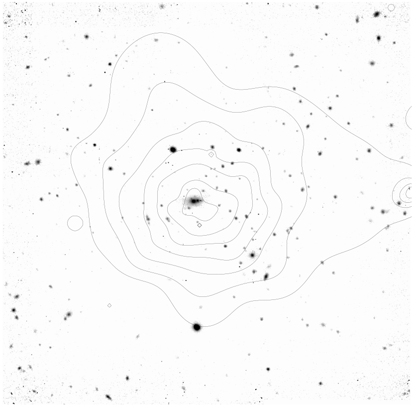
Figure 1: UKIRT UFTI $K$ band image of the $z=0.89$ cluster ClJ1226 with adaptively smoothed XMM X-ray contours from Maughan et al. (2003b). The image is $\sim 2.9$ arcmin square.

2.1.3 ClJ1415

ClJ1415.1+3612 is at the highest redshift of the three clusters with $z=1.03$ (Perlman et al. 2002). Although at present we have only ROSAT X-ray data for the cluster so sub-structure may not be resolved, it exhibits smooth X-ray contours suggesting it may be dynamically relaxed. It has a bolometric X-ray luminosity of $L_{\mathrm{X}}=2\times 10^{45}$ ergs s^-1, and is thus likely to be a very massive cluster.

2.2 Observations.

All three clusters were observed at the 3.8m United Kingdom Infrared Telescope (UKIRT) on Mauna Kea, Hawaii using the UFTI camera, a $1024\times 1024$ pixel HgCdTe array, with a pixel size of 0.091 arcseconds. Observations were made with the K98 and J98 filters (50% cut-offs 1.17–1.33$\mu$m and 2.03–2.37$\mu$m respectively) with an exposure time of 66s per frame (or 60s per frame for a minority of observations made in service time) and the seeing was typically $\approx 0.5$ arcseconds in $K$. The total exposure times in $K$ are listed in table LABEL:tab:calibration along with the average seeing for each cluster. A spatial dithering of 15 arcsec was employed. Since the field of view of 90x90 arcsec covered only a fraction of each cluster, mosaics of different sizes for each cluster were used. On each night standard stars (Hawarden et al. 2001) were observed in order to calibrate the zero-point, air mass coefficient, and colour coefficient. Some nights had patchy cloud cover, and thus yielded inaccurate photometric calibration. Such nights were deemed to be non-photometric, and a calibration was obtained via observations of the same fields on photometric nights. Non-photometric data were then weighted according to their shorter effective exposure times.

Observations were also made of one or more offset fields in the vicinity of each cluster on the sky, chosen as a reasonably ‘blank’ part of a digitised sky survey image (since at these redshifts, the clusters are also blank on digitised sky survey images). The purpose of these fields was to provide a means of estimating the contamination from foreground and background galaxies when constructing luminosity functions. The offset fields were typically 4 arcmin (1.9 Mpc) from the clusters, beyond the virial radii.

Observations of ClJ0152 were made in service time, on the nights of 15th and 20th October 2000, 24th December 2000, 28th December 2000 and 16th January 2001. The northern and southern clumps will be referred to as field A and field B. The nights of 16th January, 24th December and 28th December were found to be non-photometric and were treated accordingly. The areas observed were $1^{\prime}50^{\prime\prime}\times 1^{\prime}39^{\prime\prime}$ and $1^{\prime}51^{\prime\prime}\times 1^{\prime}50^{\prime\prime}$ for fields A and B respectively, corresponding to a physical size of $836\times 752$kpc and $843\times 836$ kpc.

ClJ1226.9+332 was observed on the 18th, 19th and 20th April 2001. The night of the 18th had patchy cloud cover and was deemed non-photometric. The observations covered an area of $2^{\prime}47^{\prime\prime}\times 3^{\prime}1^{\prime\prime}$, corresponding to a physical size of $1.3\times 1.4$ Mpc.

Cl1415 was observed on the 10th, 11th, 12th April 2002. All nights were photometric with an average seeing in K of 0.52”. The observations covered an area of $2^{\prime}2^{\prime\prime}\times 2^{\prime}44^{\prime\prime}$, corresponding to an area of $1.0\times 1.3$ Mpc. For this cluster, with the highest redshift, two offset fields were observed in order to reduce the uncertainties in the field subtraction. For the other clusters, one offset field was observed.

2.3 Data Reduction.

Each observation of a particular field consisted of a number of dithered frames of the object plus a dark frame containing only the instrumental background. The data were dark-subtracted, flat-fielded and combined using standard iraf procedures. A bad-pixel mask was applied to exclude any defective pixels. Flat-field frames were produced from the object frames, using the median value of each pixel after applying a 4$\sigma$ clipping and scaling each frame by its modal value to account for sky brightness variations.

Each frame had its background sky value subtracted, using a $3\sigma$-clipped mean as an estimate of the sky value. The relative offsets of each frame were then measured using bright stars in the field of view. Finally the frames were shifted and combined using the mean value of each pixel, again after applying a 4$\sigma$ clipping around the median value.

3 Photometry.

3.1 Standard stars.

The photometry of the galaxies was calibrated using standard stars observed on the same nights as the cluster fields. The true magnitude of any celestial body is taken to be

$$m_{{\rm true}}=ZP-2.5{\rm log}(CR)+A{\rm sec}z+B(J-K)_{{\rm true}}$$ (1)

where $ZP$ is the zero-point magnitude, $CR$ is the count rate, $A$ is the coefficient of extinction per unit airmass, $z$ is the zenith angle (sec$z$ therefore being the airmass) and $B$ is the colour coefficient necessary due to differences in the response of the combination of camera and filters used and the standard star system.

Values of $ZP$, $A$ and $B$ were determined from observations of standard stars taken on each night. Standard stars were selected from the UKIRT faint standards list (Hawarden et al. 2001). Typically each night 6 stars of varying colours were observed between 1 and 3 times each at differing airmasses.

Whilst the value of $A$ and $ZP$ may vary from night to night, the value of the colour coefficient $B$ should be almost constant. Thus a single value of $B$ was measured from all the photometric nights combined. The value we obtained is consistent with zero, as expected from the filter design (Tokunaga et al. 2002). An independent value of $ZP$ was measured for each night, and for most nights, an independent value of $A$ was measured. Where this was not possible a value of $A$ from other nights was used and checked for consistency. All were found to be consistent. In any case the low extinction in the K band and the low airmasses at which most observations were performed combine to make this a relatively small correction ($<$0.2 mag).

The parameters are listed in table LABEL:tab:calibration. Note that the final photometric error, as estimated from the scatter in the standard star measurements, is less than 0.1 mag. Corrections due to Galactic extinction are negligible ($\approx$0.007 mag) and were not applied.

Table 1: Calibration parameters for $K$ band.

	ClJ0152A	ClJ0152B	ClJ1226	ClJ1415
$A$	$-0.150\pm 0.110$	$-0.150\pm 0.110$	$-0.178\pm 0.052$	$-0.088$
$B$	$-0.0043\pm 0.094$
$ZP$	22.248$\pm 0.018$	22.248$\pm 0.018$	$22.367\pm 0.008$	22.422$\pm 0.044$
Mean sec$z$	1.445	1.403	1.210	1.160
Exposure/ s	3882	3942	23946	17820
Seeing/ arcsec	0.53	0.53	0.57	0.52

3.2 Galaxies.

The SExtractor software of Bertin & Arnouts (1996) was used to search for objects in each field. To detect objects a threshold value per pixel must be chosen along with a minimum number of connected pixels. Because the final images are constructed from a jittered pattern of images, the depth of observation varied across the final image, being at its deepest in the centres and shallowest at the edges. Therefore detection of objects was done in two regions for each image, using different detection parameters, in order to reach as deep as possible in the centre of the image whilst avoiding spurious detections at the edges of the image. Typically the minimum significance of the detections were 3.5$\sigma$ or 4$\sigma$ in the centres of the images and $7\sigma$ at the edges, where $\sigma$ is the background RMS determined from counts over the whole image (and is thus an overestimate of $\sigma$ in the central region and an underestimate in the outer region, although this is not the case for the central region of ClJ1415, when $\sigma$ was determined from the central region alone). Reliability of the object detection, and in particular the handling of overlapping objects, was checked by eye. Faint pixels surrounding deblended objects are assigned to one of the sub-objects with a probability based on the expected contribution at that pixel from each of the deblended objects (see Bertin & Arnouts 1996).

Counts were measured using an adaptive aperture based on Kron’s algorithm (Kron 1980), and also in a circular aperture with radius chosen to maximise the signal to noise. For each object a value of stellarity was also measured (see Bertin & Arnouts 1996).

To determine the magnitudes of the objects equation 1 was used with the following complication. It is unknown to start with what the true colours of the objects are, therefore the magnitudes cannot be determined. To circumvent this problem an approximate magnitude was measured in the J and K bands neglecting the colour term in equation 1. This allowed an approximate colour to be determined. The approximate colour is then multiplied by a correction factor previously determined using the same technique to measure the approximate colours of standard stars and their true colours. The average value of $\frac{(J-K)_{{\rm true}}}{(J-K)_{{\rm approx}}}$ was 0.982.

Note that for the determination of colours, magnitudes derived from fixed, circular apertures were used, whereas the adaptive aperture magnitudes were used to derive pseudo-total magnitudes. The use of adaptive aperture magnitudes using SExtractor’s Kron radius should avoid the problem described by Andreon (2002) of underestimating fluxes for galaxies with low central surface brightness. The overall reliability of the photometry was checked by comparing the field galaxy counts derived from the offset fields with deeper published results (see fig. 2). There is generally good agreement down to our limiting magnitudes (see below).

Star–galaxy discrimination was determined using SExtractor’s stellarity parameter. A cut-off of 0.8 was selected to delimit the two classes of objects with those objects with values greater than 0.8 being excluded as stars. This value was confirmed by examination of the radial profiles of detected objects. It was found that objects with a stellarity greater than 0.8 had an almost constant Gaussian FWHM close to the value of the seeing, whereas objects with stellarity less than 0.8 had more extended profiles. The results are insensitive to the precise value of this cut-off as there were very few stars in each field.

4 Luminosity functions.

K band luminosity functions (KLFs) were calculated separately for each cluster of galaxies. This was done in the following way. Firstly, some of the brightest galaxies have been spectroscopically confirmed as cluster members, so where there are no other bright galaxies in the field, no subtraction is necessary. At fainter magnitudes, the number of galaxies, $N_{\mathrm{cl}}$, in a bin of width $\Delta M$ was counted, with $\Delta M=1$ for ClJ0152 and ClJ1415 and $\Delta M=0.75$ for ClJ1226. The contamination from foreground and background galaxies was estimated by counting the number of galaxies, $N_{\mathrm{back}}$ in the offset field(s) associated with the cluster. Thus the number of galaxies in each bin is given by,

$$N_{\mathrm{bin}}=N_{\mathrm{cl}}-N_{\mathrm{back}}\times\left(\frac{A_{\mathrm{cl}}}{A_{\mathrm{back}}}\right)$$ (2)

where $A_{\mathrm{cl}}$ is the area of the cluster field and $A_{\mathrm{back}}$ is the area of the offset field. Note that because two different detection thresholds have been used for each field the faintest bins are from a smaller area than the brighter bins (since only a small area was deep enough to detect objects of this magnitude). Therefore the detections from the smaller area have been scaled by an appropriate factor to bring them into line with the detections from the total area.

The corresponding error on the number of galaxies in each bin is found by summing in quadrature the error on $N_{\mathrm{cl}}$ and the error on $N_{\mathrm{back}}$,

$$\sigma_{\mathrm{Nbin}}=\sqrt{\sigma_{\mathrm{Ncl}}^{2}+\sigma_{\mathrm{Nback}}^{2}}$$ (3)

where $\sigma_{\mathrm{Ncl}}$ is the Poissonian error (Gehrels 1986). The background error, $\sigma_{\mathrm{Nback}}$, has a Poissonian term and a term taking into account the clustering properties of galaxies, viz.,

$$\sigma_{\mathrm{Nback}}=\sqrt{N_{\mathrm{back}}}\times\sqrt{1+\frac{2\pi\it{N}A_{\omega}\theta_{\mathrm{c}}^{2-\delta}}{2-\delta}}$$ (4)

where $\it{N}$ is the number density of galaxies in the bin and $\theta_{\mathrm{c}}$ is the angular radius such that $\Omega=\pi\theta_{\mathrm{c}}^{2}$ where $\Omega$ is the solid angle of the background field. The parameters $A_{\omega}$ and $\delta$ describe the angular correlation function of galaxies such that,

$$\omega(\theta)=A_{\omega}\theta^{\delta}.$$ (5)

(Peebles 1980, pg.175).

The value of $\delta=-0.8$ was used and $A_{\omega}$ was found using the formula

$$\mathrm{log}_{10}A_{\omega}=7.677-0.3297r_{\mathrm{lim}}$$ (6)

derived by fitting to the data in table 1 of Brainerd et al. (1995). Following Djorgovski et al. (1995) we used $r_{\mathrm{lim}}-K_{\mathrm{lim}}\sim 3$.

Our limiting K magnitude was determined by plotting the number density of galaxies from the offset fields as a function of magnitude and determining the drop-off point when compared to large area field surveys. Figure 2 shows the number density of galaxies in our four offset fields. ClJ1226 and ClJ1415 were found to be complete to $K_{\mathrm{lim}}=21.5$ and ClJ0152 was found to be complete to $K_{\mathrm{lim}}=20.0$.

No corrections have been made for gravitational lensing of the background galaxies by the cluster dark matter. This effect magnifies the fluxes of background galaxies. Trentham & Mobasher (1998) show that the net increase in the number of galaxies to be subtracted is small ($<$5%) at the redshifts and magnitudes considered here (and for an equally massive cluster), because a large fraction of the field galaxies along the line of sight are in the foreground. This correction is significantly less than the statistical errors.

Figure 2: Number density of field counts as a function of magnitude. Open circles are from the combined offset fields of ClJ1226 and ClJ1415, open squares are from the offset field of ClJ0152, filled circles from Huang et al. (1997), filled squares from Saracco et al. (1997) and stars from Djorgovski et al. (1995).

Luminosity functions for the three clusters are shown in figure 3,  4 and  5 along with the best fitting Schechter functions as described below.

Figure 3: Binned K band luminosity function of ClJ0152 (z=0.83). Also shown is the best fitting Schechter function. The solid line excludes the BCGs (one from each sub-clump)and the dashed line includes the BCGs. The open symbol (offset slightly for clarity) shows the effect of excluding the BCGs from each sub-clump.

Figure 4: K band luminosity function of ClJ1226 (z=0.89). The best fitting Schechter functions including (dashed line) and excluding (solid line) the BCG are shown.

Figure 5: K band luminosity function for ClJ1415 (z=1.03). Schechter function fits are as for figure 4.

4.1 Fitting Schechter functions.

The parametric Schechter (1976) luminosity function is of the form,

$$\frac{\mathrm{d}\phi}{\mathrm{d}L}\mathrm{d}L=\phi^{*^{{}^{\prime}}}(\frac{L}{L^{*}})^{\alpha}e^{-(\frac{L}{L^{*}})}\mathrm{d}(L/L^{*})$$ (7)

where $L^{*}$ is the characteristic luminosity at which the function turns over to the faint end which has slope $\alpha$. The normalisation of the function is given by $\phi^{*^{{}^{\prime}}}$. The corresponding function in terms of K band magnitudes is

$$\mathrm{d}\phi=\phi^{*}10^{0.4(K^{*}-K)^{\alpha+1}}e^{-10^{0.4(K^{*}-K)}}\mathrm{d}K$$ (8)

where $K^{*}$ is the characteristic K band magnitude. Note that $\phi^{*}$ in equation 8 is not identical to the $\phi^{*^{{}^{\prime}}}$ in equation 7, but in fact differs by a factor $-0.4\mathrm{ln}10$.

In general the Schechter function is found to be a good fit to composite cluster galaxy LFs, as in the 2dF Galaxy Redshift Survey (De Propris et al. 2003). However, for individual clusters, there is often observed a dip in the LF (eg. Biviano et al. 1995 for the Coma cluster, Yagi et al. 2002 for a sample of 10 clusters). Biviano et al. (1995) suggest that the dip is caused by a recent episode of star-formation in the brightest galaxies thereby enhancing their luminosities. However, the presence of a dip in the $H$ band LF of Coma observed by Andreon (2002) suggests that recent star-formation is unlikely to be the cause of the dip, since the $H$ band is rather insensitive to the enhanced blue emission accompanying star-formation. Rather, Andreon (2002) suggests that the dip is the result of combining the LFs of several different types (see also Bingelli et al. 1988). However, Andreon (2002) points out that such a dip is not seen in the near-infrared LFs of five clusters studied by Trentham & Mobasher (1998), nor in the $H$ band LF of the Coma cluster measured by De Propris et al. (1998). If the dip is the result of the combination of different LFs for different morphological types, then the difference between the De Propris et al. (1998) LF and the Andreon (2002) LF suggests that the dip in the Coma LF may be dependent on which part of the cluster is being observed, and hence the particular morphological mix measured. In the present case no obvious dips are present in any of our LFs, and given the limited resolution in magnitude caused by the statistical uncertainties, the use of any functions more complicated than a Schechter function is not justified.

Equation 8 was fit to the KLFs of all 3 clusters using the maximum likelihood technique of Cash (1979). This technique fits a Schechter function to the background subtracted, binned data in the following way. The parameters $K^{*}$ and $\alpha$ are free parameters, and are allowed to vary between assumed limits. For each combination of $K^{*}$ and $\alpha$ in the parameter space, a Schechter function is calculated, with the normalisation, $\phi^{*}$, set such that the predicted number of galaxies is equal to the actual number of galaxies observed within the same magnitude limits. Thence the Cash statistic, $C$, can be computed,

$$C=-2\sum_{i=1}^{N}(n_{i}{\rm ln}e_{i}-e_{i}-{\rm ln}n_{i}!)$$ (9)

where $N$ is the number of bins, $n_{i}$ is the observed number of galaxies in the $i$th bin and $e_{i}$ is the expected number of galaxies in the $i$th bin resulting from the Schechter function. The parameters for which $C$ is a minimum are deemed to be the best fitting parameters (see Cash 1979).

It was found that $\alpha$ could not be strongly constrained and therefore, following De Propris et al. (1999) we fix at $\alpha=-0.9$ which is the value for the KLF of the Coma cluster (De Propris et al. 1998) and of the field (Gardner et al. 1997). The characteristic magnitude, $K^{*}$, was fit as a free parameter and $\phi^{*}$ was determined by ensuring that the integral of the function down to the limiting magnitude was equal to the total number of galaxies to the same magnitude.

It has been noticed since early studies of cluster luminosity functions that the brightest cluster galaxies are a special class of object (Peach 1969) and that a better fit to the LF can often be made by excluding them from the fit (Schechter 1976, Dressler 1978). Therefore Schechter functions were fit both including the BCGs and excluding them. Note that in the case of ClJ0152 we have excluded two BCGs, one from each sub-clump of the system. The best fitting parameters are given in table 2, along with the $\chi^{2}$ probability (since the maximum likelihood statistic does not give a measure of the goodness of fit). The best fitting Schechter functions, including and excluding the BCGs, are also shown in figures 3, 4 and 5.

Table 2: Best fitting parameters of a Schechter function for each cluster with $\alpha=-0.9$.

	Including BCGs			Excluding BCGs
	$K^{*}$ (lower limit, upper limit)	$\phi^{*}$	Prob($\chi^{2}$)	$K^{*}$ (lower limit, upper limit)	$\phi^{*}$	Prob($\chi^{2}$)
Cl0152	17.59 (17.26,17.90)	47.89	0.57	17.76 (17.43,18.07)	50.31	0.81
Cl1226	17.79 (17.52,18.03)	57.37	0.01	18.04 (17.79,18.28)	61.01	0.03
Cl1415	17.96 (17.63,18.26)	42.53	0.96	18.08 (17.75,18.38)	43.80	0.78
Combined	17.81 (17.51,18.07)	44.69	0.07	17.98 (17.68,18.26)	45.59	0.16

For two of the three clusters studied here, good fits are found both including and excluding the BCG (see table 2). For ClJ1226, a marginal fit is obtained excluding the BCG because of one high bin (at $K=20.4$), but the fit is poorer when the BCG is included, a conclusion supported by a visual inspection of figure 3. The values of $K^{*}$ from each cluster are consistent with each other, but are systematically fainter by $\approx$0.2 mag when the BCGs are excluded. This difference is of similar size to the statistical uncertainty. For consistency with previous measurements of Coma, in the following section we will refer to $K^{*}$ values from the fits excluding BCGs.

4.2 Evolution of $K^{*}$

To evaluate the evolution in $K^{*}$, models of galaxy evolution were made using the synthetic stellar population (SSP) libraries of Bruzual & Charlot (2003). The parameters of the model are the star formation history, the initial mass function and the metallicity. For all models considered here a single burst of star formation was assumed to occur (but at different epochs), the initial mass function was that of Salpeter (1955) and the metallicity was assumed to be solar (i.e. $Z=2\%$). Models were constructed for passive evolution in the following way. Spectral energy distributions (SEDs) were drawn from the Bruzual & Charlot (2003) libraries for different ages. A redshift of formation was chosen, corresponding to an age $t=0$. Then for the adopted cosmology redshifts were calculated for the rest of the ages. The SEDs were redshifted to the appropriate redshift for each age and multiplied by the filter transmission curve. Thus the flux of the SSP could be calculated for each redshift. The fluxes were converted to apparent magnitudes and scaled appropriately, e.g. for the evolution of $K^{*}$ the models were normalised to $K^{*}$ of the Coma cluster (see below).

No-evolution models are made by simply choosing an SED of a particular age and integrating the redshifted spectrum under the filter transmission curves.

Passively evolving models with redshifts of formation $z_{\rm{f}}=1.5$, $z_{\rm{f}}=2$ and $z_{\rm{f}}=5$ were made along with a no evolution model of a 10Gyr old population. The results are shown in figure 6. The models were scaled to the Coma cluster with $K^{*}=10.9$ at $z=0.0231$ (excluding BCGs, De Propris et al. 1999).

Figure 6: The evolution of $K^{*}$. The circles are data from this paper. The squares are from De Propris et al. (1999), open symbols being low $L_{\mathrm{X}}$ systems and closed symbols being high $L_{\mathrm{X}}$ systems.

It is clear that the trend seen in De Propris et al. (1999) is followed here and extended to higher redshifts. All values of $K^{*}$ are brighter than predicted by no evolution, and are generally consistent with passive evolution models. The high redshift points seem most consistent with $z_{f}\simeq 1.5$ although the errorbars are large enough to allow a range of $z_{f}$. A better fit to all the data would be obtained by normalising to $K^{*}$ at $z=0.2$ (which is obtained from the mean of 3 clusters) rather than normalising to Coma. In that case $z_{{\rm f}}\approx 2$ would be a better fit to the highest $z$ data.

Although it was not possible to constrain $\alpha$ for any individual cluster, in order to verify the choice of $\alpha=-0.9$ we have combined the counts from all three clusters into a general LF and fitted a Schechter function leaving $\alpha$ as a free parameter.

The combined LF was generated by finding a weighted average of the counts in each bin of the individual clusters where the weighting factor was the reciprocal of $\phi^{*}$. In fact the $\phi^{*}$ values for each cluster are similar, so the weighting has little effect. The combined LFs, excluding and including BCGs, with the best fitting Schechter functions are shown in figures 7 and 9 respectively. The best fitting values were $K^{*}=18.53$ and $\alpha=-0.54$, when the BCGs were not included and $\alpha=-0.94$ and $K^{*}=17.83$ when they were. The confidence limits, excluding BCGs, are shown in figure 8 where it can be seen that the constraint on $\alpha$ is not strong, ranging from $\alpha\approx-0.15$ – $-0.9$.

There is a large degree of degeneracy between $K^{*}$ and $\alpha$ as is evident from the shape of the contour in figure 8. Consequently when fitting a Schechter function, $K^{*}$ may be misleading if the faint end slope is poorly constrained. To quantify this effect the combined LF was fit with $\alpha=-0.9$. The results are given in table 2. The result (excluding BCGs) is a brighter value of $K^{*}$, as expected from the shape of figure 8.

Consequently, if $\alpha\approx-0.54$ for high redshift clusters then the evolution in $K^{*}$ may not be as strong as seen in figure 6, and values of $z_{f}\approx 2-5$ would be more consistent with the $K^{*}$ measurements. However, if the last bin of the combined KLF of figure 7 is excluded then $\alpha=-0.99\pm 0.4$. Thus, it is unclear whether the measured value of $\alpha=-0.54$ is in artefact due to incompleteness in the faintest bin, and therefore we elect to use the value of $\alpha=-0.9$ for the individual fits to clusters.

4.3 Comparison with the Coma cluster

We make a comparison with the Coma cluster because it has a similar $L_{{\rm X}}$ (1.6x10⁴⁵ erg s^-1), $T_{{\rm X}}$ (8 keV) and mass (10¹⁵ M_⊙) as the high redshift clusters, and it is relatively well studied at NIR wavelengths. The $K$ band LF of the Coma cluster shown in figure 7 was derived from the $H$ band luminosity function of De Propris et al. (1998) using their given value of $H-K=0.22$ and to a magnitude limit for which all galaxies had spectroscopic membership confirmation. Note that the two LFs in figure 7 have not been scaled in any way; the high redshift clusters are of similar richness as Coma (although the comparison is not exact because the high redshift LFs were obtained from a larger fraction of the cluster area than for Coma; see below). The Coma LF of Andreon & Pelló (2000) covers a smaller area than that of De Propris et al. (1998) but is in good agreement (except for a dip in one bin). For the high redshift clusters, the conversion from apparent to absolute magnitude was made using a k-correction calculated for a 10Gyr old synthetic stellar population from the libraries of Bruzual & Charlot (2003). The typical size of the k-correction was $\approx-0.7$ mag.

The offset in absolute magnitude of $K\approx$1.2 mag between the Coma KLF and the combined high redshift KLF indicates the degree of evolution. The same degree of evolution is also seen in figure 6 as the difference between the observed values of $K^{*}$ and the no-evolution predictions. Evolving the fit to the high redshift KLF, assuming a passively evolving model with $z_{\rm{f}}=2$, gives a surprisingly good description of the observed Coma KLF (the dotted lines in figures 7 & 9). Thus differences between the high redshift and low redshift systems, as shown by the bright end of the LF studied here, can be accounted for by purely passive evolution. There is no obvious change in the shape of the LFs.

Figure 7: The combined luminosity function of all three clusters ($\bar{(}z)$=0.9) shown by solid circles, excluding BCGs. Its best fitting Schechter function is the solid line, whilst the dotted line shows the expected evolution at the redshift of Coma assuming passive evolution and $z_{\rm{f}}=2$ . The number of galaxies in each bin is a weighted average. The Coma $K$ band luminosity function derived from De Propris et al. (1998) is shown by open squares. Note that the two LFs are plotted directly as observed, with no scaling. See text for details

Figure 8: Confidence limits at 68 % on the best fitting parameters for the combined luminosity function when BCGs are excluded.

Figure 9: The combined luminosity function of three clusters including BCGs. Symbols are as in figure 7.

4.4 Integrated light functions.

An interesting and complementary measure of galaxy evolution within clusters is provided by their integrated light function. This is calculated from the LF using

$${\sf j}(<L_{k})=\frac{{\displaystyle\sum_{i=1}^{k}}N_{i}L_{i}}{{\displaystyle\sum_{i=1}^{n}}N_{i}L_{i}} k=1,\ldots,n$$ (10)

where $N_{i}$ is the number of galaxies in the $i^{{\rm th}}$ bin of the LF and $L_{i}$ is the luminosity of the bin, and $n$ is the total number of bins. For the BCGs and bins in which there is only one galaxy the individual contribution was calculated using the total luminosity of the galaxy and not the bin centre.

Integrated light functions were calculated for all three clusters and for the Coma cluster. These are shown in figures 10 and 11 for data excluding and including BCGs. In order to compare each cluster the luminosity has been normalised to $L^{*}$. Thus the effects of any pure luminosity evolution (such as passive evolution), which would alter the luminosity by a constant factor, are eliminated from the plot and any variation between the shapes is due to some other evolutionary effect. Note also that in order to make this comparison the integrations of the light functions must reach the same depth below $L^{*}$. As this was not the case the counts for the faintest bin for ClJ1415 and the two faintest bins for ClJ0152 were calculated from the best fitting Schechter functions and thus these are not shown in the plots. The contribution from these bins is only 5–10% of the light integrated to our limit of $L/L^{*}=0.05$. Integrating the Schechter function to luminosities fainter than this limit would add only a further $\approx$ 1%.

Figure 10: Integrated light functions for all three clusters compared to Coma. Brightest cluster galaxies have been excluded.

Figure 11: Integrated light functions as in figure 10 but with BCGs included.

A comparison of the shapes of the integrated light functions for the four clusters excluding their BCGs, shown in figure 10, shows that they are all consistent. If the BCGs are included in the integrated light function, as in figure 11, the light functions are generally consistent within errors but the scatter is greater.

If merging plays an important role in the evolution of massive galaxies since $z\approx 0.9$ then it would be expected that there would be a higher fraction of total cluster light in bright galaxies at low redshift compared to high redshift. Little evidence is seen for this in either figure 10 or 11. If BCGs are included then ClJ1226 is seen to have a slightly higher fraction of light in its bright galaxies than Coma and ClJ0152 has a lower fraction. The lack of any systematic difference between the integrated light functions of the high redshift clusters and Coma is suggestive that merging does not play a dominant role in the evolution of massive early-type galaxies since $z\approx 0.9$.

One caveat is that interpretation of the integrated light functions is complicated by the different areas observed for each cluster. The observations of the high redshift clusters reach radii of 30%–40% of the virial radii (as measured from the X-ray properties and provided by Ben Maughan, private communication), whereas the observation of the Coma cluster covers only 0.16 of the virial radius ($r_{200}=2.3$ Mpc for $H_{0}=70$km s^-1 Mpc^-1, Reiprich & Böhringer 2002). Driver et al. (1998) show that the dwarf to giant galaxy ratio within rich clusters is strongly anti-correlated with the mean projected density outside the cores of clusters. Our observations do not, however, reach dwarf galaxy luminosities. Andreon (2001) confirms that the fraction of dwarf galaxies increases in the outer parts of a $z=0.3$ cluster, AC118, and furthermore shows that the faint end slope of the KLF recovered from the outer parts of the cluster is considerably steeper than the faint end slope of the KLF recovered from the core. Consequently comparisons of observations covering different fractions of the virial radius must be made with these effects in mind. However, our concern is with the bright end of the LF in the inner regions of the clusters, where these effects are unlikely to produce large differences.

5 The brightest cluster galaxies.

The uneasy fitting of some BCGs on the Schechter function may be symptomatic of a different evolutionary process to the majority of galaxies within a cluster. We now examine this evolution.

The K band Hubble diagram is shown in figure 12. The models are the same as described above, only now they are normalised to the low redshift ($z<0.1$), high $L_{\mathrm{X}}$ ($>1.9\times 10^{44}$ ergs s^-1 0.3 – 3.5 keV) BCG photometry of Brough et al. (2002). The high $L_{\mathrm{X}}$ clusters from figure 1 of Brough et al. (2002) are shown as the open circles. The BCGs in the current study, shown as solid points, extend to higher redshifts. Note that there are two BCGs shown for ClJ0152, one for each sub-clump. The magnitudes of the BCGs were measured in a metric aperture of radius, $r_{\mathrm{m}}=12.5h^{-1}$kpc for comparison with Brough et al. (2002). The BCG in ClJ1226 overlaps with at least one fainter galaxy observed in projection; this galaxy has been separated by Sextractor. We note that the total magnitude of the ClJ1226 BCG measured here ($K$=15.34 mag) is consistent with the isophotal value of $K$=15.5 measured by Cagnoni et al (2001).

Figure 12: K band Hubble diagram for BCGs. Solid points are from this paper, open points are from Brough et al. (2002). Magnitudes are measured within a $12.5h^{-1}$ kpc radius aperture.

It can be seen from figure 12 that the BCGs in ClJ1226 and ClJ1415 are somewhat brighter than no-evolution predictions but in good agreement with passive evolution models. The BCGs of ClJ0152 are fainter relative to the models than any other BCGs in figure 12 at $z>0.4$, perhaps indicative that the BCGs are not fully formed. Indeed as ClJ0152 is probably a merging system (Maughan et al. 2003) it may be supposed that if the BCGs merge, and no further star-formation is triggered, they will produce a brighter BCG more consistent with the other high redshift BCGs.

In contrast ClJ1226 has a relaxed X-ray morphology (Maughan et al. 2003, Ebeling et al. 2001), and is one of the brightest BCGs at $z>0.4$ relative to the models. These results are suggestive that the evolution of BCGs at high redshifts may be related to the dynamical history of the cluster they inhabit, although confirmation awaits a larger sample.

Table 3 lists the contributions from the BCG to the total $K$ band light for each cluster. The total luminosity in each cluster was calculated from the LFs, as for the integrated light functions, to a depth of $L/L^{*}\approx 0.06$. The subclumps in ClJ0152 have been treated independently, since each has a BCG. In the case of Coma a correction was made to account for the smaller fraction of the virial radius observed. This was calculated using the number density profile of Kent & Gunn (1982) to determine the ratio of the number of galaxies within the observed area to that within $0.37r_{{\rm vir}}$, the average area observed for the high redshift sample. The correction was a factor of 1.96. The luminosity of the Coma BCG, NGC4874, was calculated using the 2MASS total magnitude. Note that there are two galaxies of similar brightness in Coma, NGC4874 and NGC4884. We have taken NGC4874 as the BCG here as it resides at the centre of the X-ray emission.

Table 3: Fraction of the cluster $K$-band light in the BCGs. The values for the BCGs in ClJ0152 are the fractions in each sub-clump independently.

Cluster	Fraction	Radius/ $r_{\rm{vir}}$	$K_{{\rm BCG}}^{Tot}$
ClJ0152A	0.10	0.29	16.87
ClJ0152B	0.12	0.34	16.62
ClJ1226	0.16	0.41	15.34
ClJ1415	0.11	0.43	16.27
Coma	0.06	0.37∗	8.86

^∗ extrapolated from r=0.17$r_{\rm{vir}}$, see text.

The results show that the fraction of light in the BCGs at high redshift is greater than, or equal to, the fraction in Coma. This is still true if both brightest galaxies in Coma are included.

There are uncertainties in the corrections applied in order to compare the clusters, which were originally measured to slightly different depths and covered different areas, although the variations in radius would produce only small variations in total $K$ band light ($\sim$20% using the Coma light profile). A physical interpretation is that the high redshift BCGs are already of similar or greater mass to the BCG in Coma with no need to hypothesise any significant mergers in their future evolution.

Why are the BCGs in ClJ0152 significantly fainter than the BCG in ClJ1226? We will test the assumption that the stellar mass of the BCG is related to the mass of its host cluster. We assume the ratio of masses of the BCGs in ClJ0152 and ClJ1226 is proportional to the ratio of the total cluster masses times the ratio of the fractions of galaxy light in the BCGs, assuming the mass fraction in galaxies is the same in each cluster. Then the combined effects of the lower total mass of each subclump of ClJ0152 (by a factor of $\approx$0.39 compared to ClJ1226) and the lower fraction of cluster $K$-band light in the BCGs (by a factor of $\approx$0.69) are consistent with the difference in the luminosities of the BCGs (by 1.57 mag or a factor of 0.24). This suggests that the BCG stellar masses at high redshift may be lower in lower mass host clusters, as inferred by Brough et al. (2002), Burke et al. (2000) and Nelson et al. (2002).

We note that if the BCGs in ClJ0152 were to merge, as was hypothesised to explain their positions in the Hubble diagram, the fraction of light in the BCG would remain roughly similar.

6 Discussion and conclusions

The evolution of the galaxy populations of three high redshift clusters of galaxies has been studied. The bulk evolution of the galaxies, as characterised by $K^{*}$, is found to be consistent with passive evolution with a redshift of formation $z_{\mathrm{f}}\sim\ 1.5$–2. Further evidence for passive evolution is seen in the similarity of the shape of the high-redshift LF with that of Coma, and in the consistent shapes of the integrated light functions. Trentham & Mobasher (1998) also reached similar conclusions about the evolution of the shape of the $K$-band LF, albeit with poorer accuracy.

Purely passive evolution of early-type galaxies is consistent with several other studies including the evolution of the $K$ band luminosity function (De Propris et al. 1999), evolution of the fundamental plane in terms of mass-light ratios (van Dokkum et al. 1998), and studies of the scatter of the colour-magnitude relation (see e.g. Ellis et al. 1997, Stanford et al. 1998).

Our conclusions are different to those of Barger et al. (1998), who found no evidence of evolution in $M_{K}^{*}$ for clusters at 0.31$<$z$<$0.56 assuming a q₀=0.5 cosmology. However, the cosmological dependence is such that at these redshifts the q₀=0.5 NE prediction is very similar to the ($\Omega_{m}$=0.3, $\Omega_{\Lambda}$=0.7) $z_{f}=2$ passive evolution prediction (see e.g. figure 8 of De Propris et al. 1999). Thus the results of Barger et al. are in agreement with those found here.

When discussing formation it is important to distinguish between the epoch at which the stars in the galaxies were formed and the epoch at which the galaxies were assembled. The studies of the fundamental plane and the colour-magnitude relation refer to the epoch of star formation. If merging were a dissipationless process then it would be possible to have no extra star formation as a result of a merger and thus the age of the stars within a galaxy could be older than the age of galaxy assembly. A study of the cluster of galaxies MS 1054-03 at $z=0.83$ is presented by van Dokkum et al. (1999) and van Dokkum et al. (2000) in which there is observed a high fraction of merging red galaxies. Very little star formation is seen in the merging galaxies constituting evidence that the galaxies are in fact somewhat younger than the stars that reside within them.

Is such merging reflected in the evolution of the LF? The $K$ band luminosity of a galaxy is very nearly independent of star-formation, but reflects the mass of the old stars within the galaxy. Thus $K$ magnitudes are a good measure of the stellar mass of a galaxy. Diaferio et al. (2001) give predictions of the evolution of the KLF from semi-analytic models of dissipationless, hierarchical structure formation. The models show that there is very little evolution of the number of massive galaxies in clusters since $z=0.8$. The galaxies are assembled at high redshift and evolve passively with little subsequent merging after $z=0.8$. A detailed comparison with these models is however not possible because the luminosity evolution predictions in the models are not sufficiently accurate for massive galaxies (Diaferio et al. 2001).

It is clear from figure 6 that the bulk of galaxies in our sample were brighter in the past than predicted from no-evolution models, by $\Delta K\approx$ -1.2 mag at $z=0.9$. A direct comparison of the high-redshift $K$ band LF with that of Coma suggests that the two are very similar in shape and the differences in $M_{K}^{*}$ may be reconciled by pure luminosity evolution. The fading with time by $\Delta K\approx$ -1.2 mag is consistent with passive evolution from a formation epoch $z_{f}\approx 2$. In the monolithic collapse picture this would be expected naturally. The models of Diaferio et al. (2001) show that this is also predicted for massive cluster galaxies in a hierarchical scenario since most merging takes place early on the history of the cluster.

In a merging model passive evolutionary processes will still be present, and thus $K^{*}$ would still appear brighter than no-evolution predictions. A probe of ‘extrapassive’ processes is the shape of the LF. It is found that $\alpha$ is consistent with that of Coma although it is poorly constrained here. Perhaps a stronger test for extrapassive processes is the shape of the integrated light function. The lack of any major changes seen in figure 10 is suggestive that passive evolution alone is responsible for the evolution measured in $K^{*}$. We conclude that the luminosity evolution of bright galaxies in massive clusters is consistent with pure passive evolution, but note that this may be consistent with hierarchical models if most merging takes place at high redshifts.

The mild $K$-band evolution of luminous field galaxies to z=1 found in recent surveys is also consistent with luminosity evolution, although the amount of evolution $\Delta M_{K}^{*}=-0.54\pm 0.12$ mag (Pozzetti et al. 2003) or $\Delta M_{K}=-0.7\pm 0.3$ mag (Feulner et al. 2003, Drory et al. 2003, see also Im et al. 2002) is less than that observed here ($\Delta M_{K}^{*}=-1.2\pm 0.3$ mag) or by De Propris et al. (1999) ($\Delta M_{K}^{*}=-0.90\pm 0.25$) in massive clusters. The recent results on the field evolution indicate little change in $\phi^{*}$ to z=1, and are in contrast to the conclusions drawn by Kauffmann & Charlot (1998) and Kauffmann et al. (1996) who found evidence for a deficit of massive galaxies in the field at $z\approx 1$.

The difference in luminosity evolution between the field and massive clusters (both at z$\approx$0.9) is in the opposite sense to the environmental dependence of the formation epoch in hierarchical models (Kauffmann et al. 1993, Baugh et al. 1996, Diaferio et al. 2001). In these models, the assembly of an early-type galaxy, and the formation of its stars, occurs at an earlier epoch in a region of high overdensity than in the field. The degree of luminosity evolution between z=1 and z=0 is predicted, therefore, to be higher in early-type field galaxies than in massive clusters, since z=1 is closer to their epoch of formation. If the high redshift measurements are not in error (they can be checked via spectroscopic samples), then more detailed studies will be required to separate the $K$-band evolution of galaxies of different spectral types, since the cluster and field samples contain a different mix of galaxies and thus a different mix of star formation histories.

Note that although there is a strong case that the observed evolution in $K^{*}$ may be attributed almost entirely to passive evolutionary processes, the interpretation of this result as being due to a redshift of formation $z_{f}=1.5-2$ is less secure. The models used are for a single burst of star-formation for a stellar population with a Salpeter initial mass function having a solar metallicity. Age-redshift relations are calculated for an assumed flat cosmology with $H_{0}=70$km s^-1 Mpc^-1 and $\Omega_{\rm{M}}=0.3$ and $\Omega_{\Lambda}=0.7$. All of these assumptions affect the resultant redshift of formation and so there is clearly some slack in the interpretation of the evolution. For example if the models if figure 6 are normalised to the high $L_{{\rm X}}$ point at $z=0.2$, rather than Coma, the data are more consistent with $z_{{\rm f}}=2$–5. Future work based on the colours and morphologies of the member galaxies will provide stronger constraints on the epoch of formation.

The evolution of BCGs is consistent with that found by Brough et al. (2002) for high $L_{X}$ clusters. Figure 12 exhibits a degree of scatter in the evolution of BCGs at high redshift with some BCGs being consistent with no-evolution predictions, of which ClJ0152 is an example, and others being consistent with passive evolution. This can be interpreted as showing that some BCGs are fully formed at high redshift e.g. ClJ1226, whereas others would need to undergo merging between $z=1$ and the present to reconcile them with local BCGs.

This is supported by the ratios of $K$ band light in the BCGs to total cluster light. The ratio in Coma is not larger than the ratio in the high redshift clusters. Thus excess brightening of the BCGs with time, relative to the other cluster galaxies, as would be expected from such processes as cannibalism, is not observed, suggesting that the BCGs, at least of ClJ1226 and ClJ1415, are already fully formed.

References

- Andreon (2001) Andreon S., 2001, ApJ, 547, 623
- Andreon (2002) Andreon S., 2002, A&A, 382, 495
- Andreon & Pelló (2000) Andreon S., Pelló R., 2000, A&A, 353, 479
- Barger et al. (1998) Barger A. J., Aragon-Salamanca A., Smail I., Ellis R. S., Couch W. J., Dressler A., Oemler A., Poggianti B. M., Sharples R. M., 1998, ApJ, 501, 522
- Baugh et al. (1996) Baugh C. M., Cole S., Frenk C. S., 1996, MNRAS, 283, 1361
- Bertin & Arnouts (1996) Bertin E., Arnouts S., 1996, A&AS, 117, 393
- Bhavsar & Barrow (1985) Bhavsar S. P., Barrow J. D., 1985, MNRAS, p. 857
- Bingelli et al. (1988) Bingelli B., Sandage A., Tammann G. A., 1988, ARA&A, 26, 509
- Biviano et al. (1995) Biviano A., Durret F., Gerbal D., Le Fevre O., Lobo C., Mazure A., Slezak E., 1995, A&A, 297, 610
- Bower et al. (1992) Bower R. G., Lucey J. R., Ellis R. S., 1992, MNRAS, 254, 601
- Brainerd et al. (1995) Brainerd T. G., Smail I., Mould J., 1995, MNRAS, 275, 781
- Brough et al. (2002) Brough S., Collins C. A., Burke D. J., Mann R. G., Lynam P. D., 2002, MNRAS, 329, L53
- Bruzual & Charlot (2003) Bruzual G., Charlot S., 2003
- Burke et al. (2000) Burke D. J., Collins C. A., Mann R. G., 2000, ApJ, 532, L105
- Cagnoni et al. (2001) Cagnoni I., Elvis M., Kim D.-W., Mazzotta P., Huang J.-S., Celotti A., 2001, ApJ, 560, 86
- Cash (1979) Cash W., 1979, ApJ, 228, 939
- Cole et al. (1994) Cole S., Aragon-Salamanca A., Frenk C. S., Navarro J. F., Zepf S. E., 1994, MNRAS, 271, 781
- De Propris et al. (2003) De Propris R. et al., 2003, MNRAS, 342, 725
- De Propris et al. (1998) De Propris R., Eisenhardt P. A., Stanford S. A., Dickinson M., 1998, ApJ, 503, L45
- De Propris et al. (1999) De Propris R., Stanford S. A., Eisenhardt P. A., Dickinson M., Elston R., 1999, AJ, 118, 719
- Della Ceca et al. (2000) Della Ceca R., Scaramella R., Gioia I. M., Rosati P., Fiore F., Squires G., 2000, A&A, 353, 498
- Diaferio et al. (2001) Diaferio A., Kauffmann G., Balogh M. L., White S. D. M., Schade D., Ellingson E., 2001, MNRAS, 323, 999
- Djorgovski et al. (1995) Djorgovski S., Soifer B. T., Pahre M. A., Larkin J. E., Smith J. D., Neugebauer G., Smail I., Matthews K., Hogg D. W., Blandford R. D., Cohen J., Harrison W., Nelson J., 1995, ApJ, 438, L13
- Dressler (1978) Dressler A., 1978, ApJ, 222, 23
- Driver et al. (1998) Driver S. P., Couch W. J., Phillipps S., 1998, MNRAS, 301, 369
- Drory et al. (2003) Drory N., Bender R., Feulner G., Hopp U., Maraston C., Snigula J., 2003, astro-ph/0306299
- Ebeling et al. (2001) Ebeling H., Jones L. R., Fairley B. W., Perlman E., Scharf C., Horner D., 2001, ApJ, 548, L23
- Ebeling et al. (2000) Ebeling H., Jones L. R., Perlman E., Scharf C., Horner D., Wegner G., Malkan M., Fairley B., Mullis C. R., 2000, ApJ, 534, 133
- Eggen et al. (1962) Eggen O. J., Lynden-Bell D., Sandage A. R., 1962, ApJ, 136, 748
- Ellis et al. (1997) Ellis R. S., Smail I., Dressler A., Couch W. J., Oemler A. J., Butcher H., Sharples R. M., 1997, ApJ, 483, 582
- Feulner et al. (2003) Feulner G., Bender R., Drory N., Hopp U., Snigula J., Hill G., 2003, astro-ph/0302517
- Gardner et al. (1997) Gardner J. P., Sharples R. M., Frenk C. S., Carrasco B. E., 1997, ApJ, 480, L99
- Gehrels (1986) Gehrels N., 1986, ApJ, 303, 336
- Hawarden et al. (2001) Hawarden T. G., Leggett S. K., Letawsky M. B., Ballantyne D. R., Casali M. M., 2001, MNRAS, 325, 563
- Huang et al. (1997) Huang J.-S., Cowie L. L., Gardner J. P., Hu E. M., Songaila A., Wainscoat R. J., 1997, ApJ, 476, 12
- Im et al. (2002) Im M., Simard L., Faber S. M., Koo D. C., Gebhardt K., Willmer C. N. A., Phillips A., Illingworth G., Vogt N. P., Sarajedini V. L., 2002, ApJ, 571, 136
- Jones et al. (1998) Jones L. R., Scharf C., Ebeling H., Perlman E., Wegner G., Malkan M., Horner D., 1998, ApJ, 495, 100
- Kauffmann & Charlot (1998) Kauffmann G., Charlot S., 1998, MNRAS, 297, L23
- Kauffmann et al. (1996) Kauffmann G., Charlot S., White S. D. M., 1996, MNRAS, 283, L117
- Kauffmann et al. (1993) Kauffmann G., White S. D. M., Guiderdoni B., 1993, MNRAS, 264, 201
- Kent & Gunn (1982) Kent S. M., Gunn J. E., 1982, AJ, 87, 945
- Kron (1980) Kron R., 1980, ApJS, p. 305
- Maughan et al. (2003) Maughan B. J., Jones L. R., Ebeling H., Perlamn E., Rosati P., Frye C., Mullis C. R., 2003, ApJ, in press (astro-ph/0301218)
- Maughan et al. (2003) Maughan B. J., Jones L. R., Scharf C. A., Ebeling H., Barrett E., 2003, in preparation
- Nelson et al. (2002) Nelson A. E., Gonzalez A. H., Zaritsky D., Dalcanton J. J., 2002, ApJ, 566, 103
- Peach (1969) Peach J. V., 1969, Nature, 223, 1140
- Peebles (1980) Peebles P. J. E., 1980, The Large-Scale Structure of the Universe.. Princeton University Press, Princeton, NJ
- Perlman et al. (2002) Perlman E. S., Horner D. J., Jones L. R., Scharf C. A., Ebeling H., Wegner G., Malkan M., 2002, ApJS, 140, 265
- Pozzetti et al. (2003) Pozzetti L., Cimatti A., Zamorani G., Daddi E., Menci N., Fontana A., Renzini A., Mignoli M., Poli F., Saracco P., Broadhurst T., Cristiani S., D’Odrico S., Giallongo E., Gilmozzi R., 2003, astro-ph/0302599
- Reiprich & Böhringer (2002) Reiprich T. H., Böhringer H., 2002, ApJ, 567, 716
- Salpeter (1955) Salpeter E. E., 1955, ApJ, 121, 161
- Sandage (1972a) Sandage A., 1972a, ApJ, 173, 485
- Sandage (1972b) Sandage A., 1972b, ApJ, 178, 1
- Saracco et al. (1997) Saracco P., Iovino A., Garilli B., Maccagni D., Chincarini G., 1997, AJ, 114, 887
- Scharf et al. (1997) Scharf C., Jones L. R., Ebeling H., Perlman E., Malkan M., Wegner G., 1997, ApJ, 477, 79
- Schechter (1976) Schechter P., 1976, ApJ, 203, 297
- Stanford et al. (1998) Stanford S. A., Eisenhardt P. R., Dickinson M., 1998, ApJ, 492, 461
- Tokunaga et al. (2002) Tokunaga A. T., Simons D. A., Vacca W. D., 2002, PASP, 114, 180
- Trentham & Mobasher (1998) Trentham N., Mobasher B., 1998, MNRAS, 299, 488
- van Dokkum et al. (2000) van Dokkum P. G., Franx M., Fabricant D., Illingworth G. D., Kelson D. D., 2000, ApJ, 541, 95
- van Dokkum et al. (1999) van Dokkum P. G., Franx M., Fabricant D., Kelson D. D., Illingworth G. D., 1999, ApJ, 520, L95
- van Dokkum et al. (1998) van Dokkum P. G., Franx M., Kelson D. D., Illingworth G. D., 1998, ApJ, 504, L17
- Visvanathan & Sandage (1977) Visvanathan N., Sandage A., 1977, ApJ, 216, 214
- Yagi et al. (2002) Yagi M., Kashikawa N., Sekiguchi M., Doi M., Yasuda N., Shimasaku K., Okamura S., 2002, AJ, 123, 87