TURBULENCE IN CLUSTERS OF GALAXIES AND X-RAY LINE PROFILES

N.A. Inogamov^1,2 and R.A. Sunyaev^2,3

¹ Landau Institute for Theoretical Physics, Russian Academy of Sciences, Chernogolovka, Russia

² Max-Planck-Institut für Astrophysik, Garching, Germany

³ Space Research Institute, Russian Academy of Sciences, Moscow

Full text of the paper will be published in December, 2003 issue of Astronomy Letters 29, 791.

Abstract Large-scale bulk motions and hydrodynamic turbulence in the intergalactic gas inside clusters of galaxies significantly broaden X-ray emission lines. For lines of heavy ions (primarily helium-like and hydrogen-like iron ions), the hydrodynamic broadening is significantly larger than the thermal broadening. Since cluster of galaxies have a negligible optical depth for resonant scattering in forbidden and intercombination lines of these ions, these lines are not additionally broadened. At the same time, they are very intense, which allows deviations of the spectrum from the Gaussian spectrum in the line wings to be investigated. The line shape becomes an important indicator of bulk hydrodynamic processes because the cryogenic detectors of new generation of X-ray observatories will have a high energy resolution (from 5 eV for ASTRO-E2 to 1-2 eV for Constellation-X and XEUS). We use the spectral representation of a Kolmogorov cascade in the inertial range to calculate the characteristic shapes of X-ray lines. Significant deviations in the line profiles from the Gaussian profile (shape asymmetry, additional peaks, sharp breaks in the exponential tails) are expected for large-scale turbulence. The kinematic SZ effect and the X-ray line profile carry different information about the hydrodynamic velocity distribution in clusters of galaxies and complement each other, allowing the redshift, the peculiar velocity of the cluster, and the bulk velocity dispersion to be measured and separated.

Key words: turbulence, clusters of galaxies, intergalactic gas, X-ray line spectroscopy.

1 The General Picture

The hot intergalactic gas in clusters of galaxies forms an extended atmosphere in the gravitational potential well produced mainly by the weakly interacting dark matter, whose mass exceeds the intergalactic gas mass by a factor of approximately six. The cluster gas temperature reaches 2-10 KeV. The speed of sound in this gas is 1000-1500 km s${}^{-1}.$ Galaxies move through the cluster gas with subsonic, sonic and supersonic velocities. Energetically, the presence of galaxies is of little importance, because the total mass of the galaxies is appreciably smaller than the total cluster mass. The intergalactic gas consists of completely ionized hydrogen together with $\sim$ 25 % (by mass) of helium. Heavy elements, including iron, are represented at a 30 - 40% level of their solar abundance.

Due to the growth of large-scale cosmological density perturbations, clusters of galaxies sometimes merge together and capture surrounding galaxies and groups of galaxies. During such merger, the colliding components move with supersonic or transonic velocities. Each merger is accompanied by shock wave formation and turbulence generated on smaller scales. The characteristic time between mergers is long. The effects of no more than one to three large mergers appear to be observed simultaneously; a large merger is a merging of clusters with comparable masses. The capture of low-mass companions or individual galaxies gives a smaller contribution to the generation of turbulence.

It follows from $N$-body simulations with cold dark matter and gas that the turbulent pressure can account for up to 15% of the thermal pressure of the intergalactic gas in relaxed clusters of galaxies. This value implies very high turbulent pulsation velocities (up to 40% of the speed of sound). Remarkably, the calculations by different groups yield similar results (the methods, codes, and results were carefully compared by Frenk et al. 1999; see also Norman and Bryan 1999).

Activity of accreting supermassive black holes in the dominant galaxy inside the cluster can trigger additional small-scale turbulence due to existence of collimated high-velocity mass outflows and interaction of intergalactic gas with relativistic jet (Churazov et al. 2002a, 2002b).

1.1 X-ray Line Profiles

In 2005, ISAS and NASA are planning to launch the ASTRO-E2 satellite. This satellite will be equipped with cryogenically cooled X-ray bolometers. They will be placed in the focal planes of grazing-incidence telescopes. The expected energy resolution will be $\sim$ 5 eV (FWHM) in the photon energy range from 0.5 to 10 keV, which includes the line of the helium-like iron ion (the iron ion with two electrons) at energy 6.7 keV. Since below we compare the line profiles with Gaussian fits, it is important to note (Porter and Mitsuda 2003) that this resolution corresponds to a dispersion of 2.7 eV. The prospective Constellation-X and XEUS missions will have X-ray detectors with an energy resolution as high as 1-2 eV. Therefore, it will become possible to detect line shifts and broadenings in rich cluster of galaxies that correspond to turbulent velocities $\sim$ 3 $\times$ 10^-4 of the speed of light, i.e. up to 100 km s^-1 or less than 10% of the speed of sound.

During turbulent pulsations, iron ions move in a mixture with hydrogen and helium nuclei. Accordingly, all ions have the same hydrodynamic velocities. The thermal velocities of ions of different types with the same temperature greatly differ because of the large difference between the nuclear masses. Therefore, the Doppler turbulent broadening of iron lines $\Delta E/E\sim v_{\rm turb}/c$ can significantly exceed their thermal broadening. The thermal velocity of iron ions is $\sim\sqrt{m_{p}/m_{Fe}}=1/\sqrt{56}$ = 13% of the speed of sound, where $m_{p}$ and $m_{Fe}$ are the masses of the proton and the iron atomic nuclei, respectively. The amplitude of the turbulent velocity pulsations produced by a cluster merger can exceed the thermal velocities of iron ions several fold. Thus, iron ions become effective tracers of turbulent velocity fields in the cluster interiors.

Let us introduce the parameter

$$\mathop{\rm Ma}\nolimits_{i}=\frac{u_{\rm rms}}{\sqrt{kT/m_{i}}}=\sqrt{2}\,\frac{\Delta\nu_{\rm DH}}{\Delta\nu_{\rm DT}}=4.2\,\frac{u_{\rm rms}}{300\,[\,\rm{km\;s^{-1}}\,]}\,\sqrt{\frac{3\,[\rm keV]}{kT}}\,\sqrt{\frac{m_{i}}{56\,m_{p}}}$$

that characterizes the ratio of the turbulent ($v_{\rm turb}\sim u_{\rm rms}$) and thermal velocity scales for an ion of mass $m_{i}$. It resembles the Mach number: $Ma=u_{\rm rms}/c_{s}$ (the ionic Mach number), where $c_{s}$ is the speed of sound. Parameter (1.1) defines the ratio of the hydrodynamic ($\Delta\nu_{\rm DH}$) and thermal ($\Delta\nu_{\rm DT}$) Doppler broadenings:

$$\Delta\nu_{\rm DH}=\nu_{0}\,\frac{u_{\rm rms}}{c},\;\;\;\;\;\Delta\nu_{\rm DT}=\nu_{0}\,\frac{\sqrt{2kT/m_{i}}}{c}.$$

In (1.1) and (1.2) $u_{\rm rms}$ is the line-of sight or radial hydrodynamic velocity dispersion and $\nu_{0}$ is the frequency at the center of the line profile.

The most intense lines observed in the spectral range between 2 and 10 keV are those of helium and hydrogen-like iron ions. The equivalent width of the most intense iron lines reaches 100-500 eV. At the thermal Doppler width of $\sim$ 3 eV, they must rise by tens and hundreds of times above the smooth continuum associated with hydrogen-helium plasma bremsstrahlung. XMM observations of the central part of the Perseus cluster of galaxies gave 10⁵ photons in 50 ks in the complex of iron K-lines near 6.7 keV (Churazov et al. 2003). The Constellation-X and XEUS satellites will have an effective area that is tens of times larger than that of XMM, which will make it possible to study in detail the weak wings of X-ray lines.

The spectral surface brightness of a cluster in a line is given by the formula

$$I(\Delta E,y,z)=\int dx\,j[E_{0},T_{e}(x,y,z)]\,n_{e}(x,y,z)\,\frac{dn_{i}(x,y,z,\Delta E)}{d(\Delta E)},$$

where $I$ is measured in photons cm^-2 s^-1 eV^-1 (square angular minute)${}^{-1},$ the emissivity coefficient $j$ characterizes the rate of production of excited ions and emission of photons with energy $E_{0}$ by these ions, $n_{e}$ is the electron density, and $dn_{i}/d(\Delta E)$ is the number of ions of a given type in the range of velocities that shift the line photons to the energy range from $\Delta E{\rm to}\Delta E+d(\Delta E$) (in the frame of reference associated with the ion, the photon energy is $E_{0},$ without Doppler and intrinsic broadenings). The energy $\Delta E=E-E_{0}$ is measured from the line center and is proportional (see below) to the line-of-sight ion velocity. The line-of-sight velocity of ions can be determined by taking into account their thermal and hydrodynamic velocities. We assume that the thermal velocity distribution of ions is Maxwellian with an ion temperature equal to the electron temperature. The hydrodynamic velocity distribution can be calculated in terms of the turbulence model presented below. In the above formula, the natural line width is disregarded (see formulas (12.2) - (12.5) in the full paper). Emissivity coefficient $j$ depends on the electron temperature $T_{e}.$ In an isothermal plasma at a constant (in volume) elemental abundance, $n_{e}n_{i}\propto n_{e}^{2}.$

In this paper, we consider qualitative effects, primarily the line broadening, its spectral shift due to bulk and turbulent motions and the degree of deviation of the emission line profile from the Gaussian profile. Therefore, for illustration, we investigate the simplest case of an isothermal cloud with constant density and elemental abundance over its volume. In this case, the above formula for the brightness $I$ takes the form

$$I(\Delta E,y,z)=j(E_{0},T_{e})\,n_{e}\int dx\,\frac{dn_{i}(\Delta E)}{d(\Delta E)}=\alpha\,j\,n_{e}^{2}\,\int dx\,\psi(x,y,z,\Delta E),$$

where $\alpha$ is the elemental abundance, and the function $\psi$ specifies the local line-of-sight velocity distribution. We ignore the nonlinear density variations due to turbulent pulsations.

An efficient method for solving the problem of the iron line profile involves direct numerical simulation. The first attempt of this kind was made by Sunyaev, Norman, and, Bryan (2003). Below, we attempt to construct a relatively simple turbulence model (see formula (4.1) below) to understand in which cases the shape of a turbulently broadened line can differ from the Gaussian shape expected from the central limit theorem of the probability theory. The model is based on the assumption about a Kolmogorov cascade in the inertial range limited by the mixer size $L_{\rm mix}$ and the viscous scale $L_{\nu}$. The number of mixers in the large-scale case ($L_{\rm mix}\sim L$) is limited. As a result, the line spectrum significantly deviates from the Gaussian spectrum.

Fig. 1 shows the characteristic profile of the helium-like iron (Fe XXV) permitted $w-$line (curve 4) obtained in the adopted model. As we see (cf. curves 2 and 4), there are qualitative deviations from the commonly assumed Gaussian line profile

$$\frac{u_{\rm rms}\exp\left[-(1/2)\,u^{2}/(u_{rms}^{2}+kT/m_{i})\right]}{\sqrt{2\pi}\,\sqrt{u_{rms}^{2}+kT/m_{i}}}=\frac{(2\pi)^{-1/2}}{\sqrt{1+\mathop{\rm Ma}\nolimits_{i}^{-2}}}\,\exp\left(-\frac{(1/2)\,\hat{u}^{2}}{1+\mathop{\rm Ma}\nolimits_{i}^{-2}}\right)$$

with a dispersion the square of which is equal to the sum of the squares of the thermal and hydrodynamic dispersions (curve 2). In what follows

$$\hat{u}=u/u_{\rm rms},\;\;\;\Delta E[\rm eV]=-6.7\,[\rm eV]\,(u_{\rm rms}/300[{\rm km\,s^{-1}}])\,\hat{u},$$

$\hat{u}$ is a dimensionless velocity (in units of dispersion), and $\Delta E$ is the deviation from the profile center. Formula (1.3) is used to recalculate $\hat{u}$ to $\Delta E$. Parabola 1 in Fig 1 corresponds to the Maxwellian distribution of ions $f_{T}(\hat{u})=(Ma_{i}/\sqrt{2\pi})\exp(-\mathop{\rm Ma}\nolimits_{i}^{2}\,\hat{u}^{2}/2$) (purely thermal broadening). All distributions where normalized to unity $\int^{\infty}_{-\infty}f(\hat{u})d\hat{u}$ = 1. Curves 3, $f_{\rm HT}(\hat{u}$), and 4, $f_{\rm HTL}(\hat{u}$), represent the turbulent line profiles. The distribution $f_{\rm HT}(\hat{u}$) includes hydrodynamic (H) and thermal (T) broadenings, while the distribution $f_{\rm HTL}(\hat{u}$) includes hydrodynamic, thermal, and Lorentz (L) broadenings. The intrinsic or Lorentz broadening was calculated for the Fe XXV $w-$line.

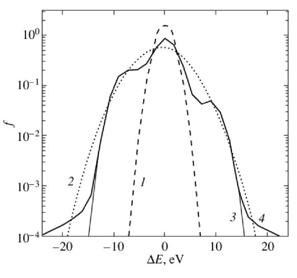
Figure 1: Fe XXV $w$-line spectrum (4) at $kT$ = 3 keV; 1 – the thermally broadened line profile (without hydrodynamic broadening), 2 – the Gaussian profile with a total (hydrodynamic plus thermal) dispersion $u_{\rm HT}$ = 190 km s^-1, and 3 – the line profile without Lorentz broadening.

Fig. 2 shows, first, the computed spectra (fluctuating solid curves), second, the thermal Gaussians of the helium-like iron $w$-line (dashed curves, narrow parabolas), and, third, the Gaussian fits to the computed spectra (long0dashed wide parabolas). These spectra were constructed for nine points of the cluster projection onto the plane of the sky. The Gaussian fits are specified by two parameters (shift $u_{1}$ and broadening $u_{\rm HT})$ that can be determined from the computed spectrum (see Table 1). These nine columns correspond to the center, vertices, and middles of the sides of the square in the plane of the sky described in Sections 1.2 and 1.3, see also Section 11 of the full paper. Note that curve 3 in Fig. 1 corresponds to the line profile shown in the middle panel in the upper row of Fig. 2.

Fig. 3 (a) shows the radiation spectrum for a hot plasma with a temperature of 3 keV and a normal chemical abundance in the energy range near the permitted helium-like iron line at $\approx$ 6.7 keV. The complex of iron lines near the hydrogen-like iron line ($E_{0}\approx$ 6.9 keV) is shown in Fig. 3 (b) at $kT$ = 8 keV. These plots show the individual lines in the form of narrow peaks with a width close to 10^-2 eV. The plots were constructed by using the APEC code (Astrophysical Plasma Emission Code; Smith et al. 2001), which is part of the XSPEC V11.2 code. All lines were normalized to the most intense permitted $w$-line ($E_{0}$ = 6.7005 keV). As an illustration, the dashed curves in Fig. 3 (a) and (b) indicate the same spectra broadened by thermal motions of the ions.

Fig. 4 (a)–(c) show the complex of lines near 6.7 keV taking into account both thermal and hydrodynamic motions. These spectra were computed by folding the profiles presented in the upper middle, central, and lower left panels of Fig. 2 with the complex of individual lines and satellites shown in Fig. 3 (a). The dashed curves again represent the broadening of the individual lines due to thermal ion motions in the absence of hydrodynamic motions.

The solid and dashed curves in Figs. 4 (a)–(c) were normalized to the same number of photons in the whole complex of lines.

The plasma emission is a function of the temperature. An increase in temperature affects both the relative line intensity and the thermal line width. At high temperatures (e.g., $kT$ = 8 keV), the complex of hydrogen-like iron lines near energy 6.9 keV becomes intense, Fig. 3 (b).

Figure 2: Helium-like iron line profiles at nine points in the image of a cluster with $kT$ = 3 KeV. The solid curves represent line profiles shifted and broadened due to hydrodynamic and thermal motions and the dashed curves (narrow parabolas) specify the thermal line broadening. The hydrodynamic and thermal velocity dispersions and the velocity corresponding to the shift of the line profile centroid are given in Table 1 for each of the nine lines. The long-dashed curves (wide parabolas) represent the Gaussian fits to the computed spectra.

Using Figs. 3 (a) and (b), we wish to emphasize the following. The most favorable energy range for observing hydrodynamic iron line broadening effects is to the right of the $w$-line center, because there are virtually no other intense lines at $kT$ = 3-10 keV within several tens of eV of the center of this line. Thus, the far wings of the broadened line can be studied in detail.

Of considerable interest is also the iron $z$-line at photon energy $E_{0}$ = 6.6366 keV that corresponds to the transition from the 1s2s triplet to the ground state: ${}^{3}S\rightarrow^{1}S$. In this case, the left line wing is favorable for observations. It is possible to simulate the spectrum of the entire set of lines in both complexes and to compare it with the observed spectrum.

Figure 3: Spectra for the complexes of iron lines near 6.7 keV at $kT_{e}$ = 3 keV (a) and near 6.9 keV at $kT_{e}$ = 8keV (b). The dashed curves specify the thermal broadening of the lines. The lines were normalized to the most intense permitted helium-like iron $w$-line.

Fig. 4 (c) shows a very large shift of the line observed from the column in the lower left panel in Fig. 2. All of this column flies toward us. The velocity dispersion in it slightly exceeds the thermal velocity dispersion. In contrast, the upper right panel of Fig. 2 shows that the corresponding column flies away from us with a slightly lower radial velocity and larger velocity dispersion. Collectively, these two panels suggest the presence of a large-scale motion similar to the rotation of the entire cluster gas – this is a manifestation of a large-scale mixer, i.e., the last large merger.

In the central part of the cluster (Figs. 2 and 4 (b)), the broadening and the shift are so large that the individual lines and satellites in the complex of lines are barely discernible.

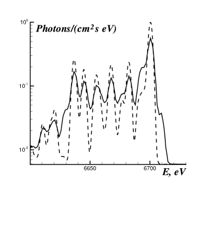
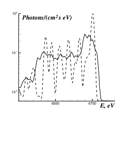
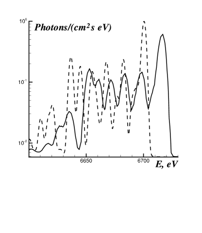
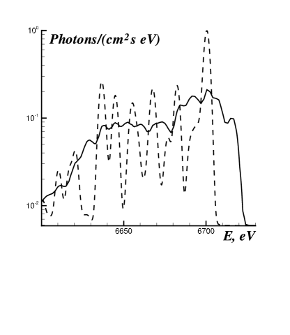
Figure 4: (a,b,c) Spectra for the complex of iron lines near 6.7 keV for $kT_{e}$ = 3 keV are obtained by folding with the profiles shown in the upper middle, central, and lower left panels of Fig. 2, respectively. The dashed curves specify the spectrum for the thermally broadened lines of the complex. All curves were normalized to the same total number of photons in the complex of lines. (d) An approximate spectrum for the complex of iron lines near 6.7 keV from the cluster as a whole obtained by folding the profile in Fig. 5 with the spectrum in Fig. 3 (a).

Table 1. Shifts and broadening of the X-ray line profile at $E_{0}$ = 6.7 keV. The positions of the cells in the table and the data in them correspond to the spectra of the nine line-of-sight columns presented in Fig. 2. The fourth row of the table gives the velocity dispersion for the cluster as a whole. This is dispersion of the integrated spectrum in Fig. 5. In the Table, $u_{1}$ is the shift of the line profile center in [km s^-1], and $u_{\rm HT}$ is the dispersion of the computed distributions from Fig. 2.

$u_{1},\;u_{\rm HT}$	$+180,\;330$	$-39,\;190$	$-450,\;200$
$u_{1},\;u_{\rm HT}$	$+205,\;165$	$-205,\;280$	$-470,\;190$
$u_{1},\;u_{\rm HT}$	$+695,\;110$	$+440,\;180$	$+80,\;140$
$u_{1},\;u_{\rm HT}$		$0,\;460$

Since the ASTRO-E2 spectrometers have a limited angular resolution, they will yield detailed images only for the nearest rich clusters of galaxies. For distant clusters, the line profiles from the entire cluster will be investigated. Figs. 4 (d) and 5 give the first idea of this profile. A comparison of Fig. 4 (d) with Figs. 4 (a)–(c) shows how informative the set of high resolution spectroscopic data is even with a limited angular resolution. The profile in Fig. 5 was obtained by averaging the nine profiles presented in Fig. 2 with equal statistical weights. Recall that each of these nine profiles was obtained for a very narrow unit column in a cube with a volume of 160³ mesh points. Clearly, the line profile from the entire cube must be even smoother. On the other hand, the shifts of the profiles shown in Fig. 2 and Table 1 suggest the presence of intense large-scale motions inside the cluster. In observations of the cluster as a whole, they give a large contribution to the dispersion but must leave traces in high-energy-resolution spectra. The profile in Fig. 5 is much broader than any of the nine profiles in Fig. 2 (see Table 1); in particular, it is broader than the profile in Fig. 1. This is the result of large-scale motions.

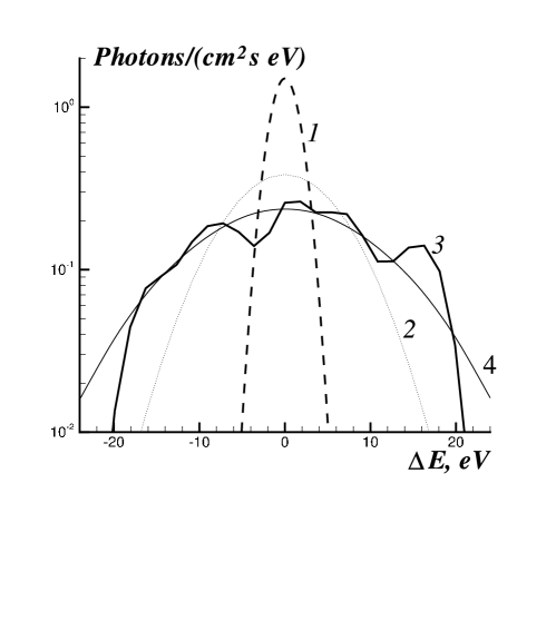
Figure 5: The iron line profile (curve 3) at $E_{0}=6.7$ keV obtained by summing the nine profiles shown in Fig. 2. This profile was also normalized to the total number of photons. To a first approximation, this profile corresponds to the line profile observed from the entire cluster. The thermal broadening (curve 1) and the two Gaussian curves for the total broadening in the entire cluster (total dispersion 460 km s^-1, curve 4) and for dispersion $u_{\rm rms}$ = 270 km s^-1 (curve 2) corresponding to the central panel in Fig. 2 are shown for comparison.

The spectrum in Fig. 4 (d) was obtained by folding the profile in Fig. 5 with the complex of iron lines near 6.7 keV shown in Fig. 3 (a). We see individual spectral features, but their amplitude is appreciably smaller than that predicted in the model with thermal broadening and a smaller hydrodynamic velocity dispersion. The high-energy wing of the permitted helium-like iron $w$-line makes it possible to judge the total velocity dispersion in the cluster.

The turbulent broadening determined for all the nine profiles shown in Fig. 2 corresponds to a large (at least severalfold) decrease of the optical depth in the resonance $w$-line. That is why we disregard the broadening of this line due to resonant scattering (Gilfanov et al. 1987) in the plots of Fig. 2–5.

To elucidate the turbulence model, Fig.6 shows a Kolmogorov spectrum of the Fourier velocity amplitudes $u_{n}$ with a power-law scaling in the wavelength range $L_{\nu}<\lambda<L_{\rm mix}\leq L$ and harmonic numbers $1\leq N_{\rm mix}<n<N_{\nu}$, where$L$ is the cluster scale, $\lambda=\lambda_{n}=L/n,\,$ $k=k_{n}=2\pi/\lambda_{n}=2\pi n/L,\,$ $N_{\rm mix}=L/L_{\rm mix},\,$ $N_{\nu}=L/L_{\nu}$, and $L_{\nu}$ is the viscous damping scale. Note that the total number of energy-containing eddies in volume $L^{3}$ is $N_{\rm mix}^{3}$. Below, we show that the velocity dispersion and the hydrodynamic Doppler broadening (1.2) are determined by large-scale fluctuations with $\lambda\sim L_{\rm mix}$. The fractal line profile fluctuations, which are smoothed out by thermal broadening, are associated with the Kolmogorov small-scale tail.

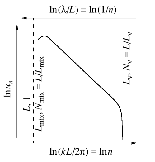
Figure 6: The $\lambda$ and $k$ fluctuation spectrum in a Kolmogorov model. The scales ($L$,1), ($L_{\rm mix},N_{\rm mix}$), and $(L_{\nu},N_{\nu})$ characterize the cluster, the turbulence-maintaining mixers, and the viscous dissipation region, respectively.

When computing the realization shown in Figs. 1–5, we took $N_{\rm mix}$ = 1 and $N_{\nu}$ = 40. Because of the significant thermal broadening of the profile and the decrease in small-scale pulsation velocity amplitude with decreasing scale, the difference between the realizations for $N_{\nu}$ = 40 and $N_{\nu}\gg$ 40 is small (see the full paper for a discussion). The dependence on $N_{\rm mix}$ is discussed in Section 7 below.

We calculated the velocity field $u(x,y,z)$ in a cube $(2l)^{3}$ with an edge 2$l$. The function $u(x,y,z)$ satisfies periodic boundary conditions at the boundaries of the large cube $L^{3}$. In our calculations (Figs. 1-5), we took $L=1$ and 2$l$ = 0.4. We chose 2$l<L$ to reduce the influence of the periodic boundary conditions. The cube $(2l)^{3}$ was covered by a 3D mesh of 160³ computational points. The separations between the mesh points are $\delta l=2l/160$. Each column in Fig. 2 has a length 2$l$ along the line of sight and a cross section in the plane of the sky in the form of a $\delta l\times\delta l$ square.

1.2 Turbulence and the Kinematic SZ Effect

The hydrodynamic velocity distribution of a cluster in the plane of the sky can also be analyzed by studying manifestations of the kinematic SZ effect (Sunyaev and Zeldovich 1980), i.e. by measuring the intensity fluctuations of the cosmic microwave background radiation (CMB) within the cluster

$$\frac{\Delta T_{r}(y,z)}{T_{r}}=\sigma_{T}\,\int_{-\infty}^{\infty}\,\frac{v_{||}(x,y,z)}{c}\,n_{e}(x,y,z)\,dx.$$

Sunyaev et al. (2003) and Nagai et al. (2003) used this method of analysis in their numerical modeling. Formula (1.4) was first suggested by Sunyaev and Zeldovich (1970) to calculate the primordial Doppler CMB fluctuations and was used by Sunyaev (1977) in calculating the fluctuations due to secondary ionization. In formula (1.4), $y$ and $z$ are the coordinates in the plane of the sky; $x$ is the coordinate along the line of sight; and $v_{||}$ is the component of the local hydrodynamic velocity vector along the line of sight (the $x$ velocity component) below denoted by $u$, $\hat{v}_{||}=v_{||}/u_{\rm rms};$ and $T_{r}$ is the CMB temperature. The $\Delta T_{r}/T_{r}$ fluctuations (1.4) differ only by a factor from the fluctuations in the dimensionless total momentum

$$p(y,z)=\int\,\hat{n}_{e}\,\hat{v}_{||}(x,y,z)\,dx/(2l),$$

of the emitting matter along the $x$ axis (the line-of-sight or column momentum), where $\hat{n}_{e}=n_{e}/(n_{e})_{\rm centr},$ $(n_{e})_{\rm centr},$ is the central cluster density. Below, the density $n_{e}$ is assumed to be roughly uniform over the cluster core.

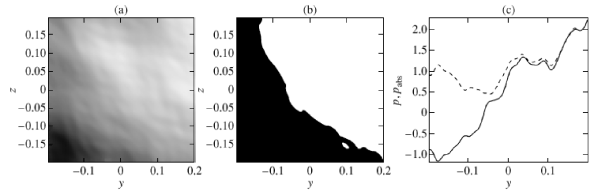
Figure 7: Distribution of the CMB intensity fluctuations (1.4) in the $y,z$ plane of the sky that follows from the Kolmogorov model. (a) A map of the line-of sight momentum $p(y,z);\,$ $L=1$. The white and black colors correspond to the motion away from and toward the observer, respectively. The shades of gray give the local values of $\Delta T_{r}(y,z)/T_{r}.$ (b) The $\Delta T_{r}(y,z)/T_{r}=0$ isoline that separates the black and white regions with opposite signs of $\Delta T_{r}.$ (c) The $p(y,z=0)$ cut (solid curve) of the $p(y,z)$ surface. Dashed line represents the same cut in the case of the function $p_{\rm abs}$ given by formula (1.6).

Fig. 7 and 8 show maps, reliefs, and cuts of the intensity fluctuations (1.4). The degree of blackening in Fig. 7 (a) is proportional to the local $\Delta T_{r}(y,z)/T_{r}$ fluctuation amplitude and the local momentum $p(y,z)$. Fig. 7 (b) shows regions in the $y,z$ plane of the sky that move toward (black) and away from us (white). We performed our calculations by using the Kolmogorov model (for details, see the sections below). For long-wavelength turbulence with $N_{\rm mix}\sim 1$ (see Fig. 6), the size of the region with the same sign of $p$ (1.5) is on the order of the cluster size $L$. In the typical realization shown in Figs. 1-5 and 7-10, $N_{\rm mix}$ = 1 and $N_{\nu}$ = 40. Fig. 7 (c) shows the cut of the $p(y,z)$ surface (see Fig. 8) by the $z=0$ plane that passes through the cluster center. The solid and dashed curves in this figure indicate, respectively, the functions $p(y,0)$ (1.5) and

$$p_{\rm abs}(y,0)=\int_{-l}^{l}\,\hat{n}_{e}\,|\hat{u}(x,y,0)|.\,dx/(2l)$$

In the large-scale case ($N_{\rm mix}\sim 1$), the functions $|p(y,z)|$ (1.5) and $p_{\rm abs}(y,z)$ (1.6) are of the same order of magnitude, as illustrated by Fig. 7 (c).

The sizes of the identically signed spots (Fig. 7 (b) for the function $p(y,z)$ and the $|p|/p_{\rm abs}$ ratio are determined by the scale $L_{\rm mix}=L/N_{\rm mix}$. If there are many mixers ($N_{\rm mix}\gg 1$), then the function $p(y,z)$ changes sign during a displacement $\Delta l_{\perp}\sim L_{\rm mix}$ in the plane of the sky transverse to the line of sight. In this case, $|p|/p_{\rm abs}\sim 1/\sqrt{N_{\rm mix}}$. In deriving these estimates, we assume that (1) the separation between mixers is on the order of their size, (2) the fluctuation amplitude of the velocity $u_{\rm rms}$ on each mixer is of the same order of magnitude, and (3) the velocity correlation decays on a scale on the order of $L_{\rm mix}$. In this case $p_{\rm abs}\sim 1$, because $\langle\hat{u}\rangle\sim 1,$ $\langle 2l\rangle\sim 1$ (we set $\hat{n}_{e}$ = 1), and $|p|\sim N^{-1/2}_{\rm mix}$, because the total momentum $p(y,z)$ (1.5) along the $x$ line of sight is the sum of the momenta of $N_{\rm mix}$ out-of-phase mixers.

It is interesting to calculate the Kolmogorov scaling law for the CMB fluctuations $\Delta T_{r}/T_{r}\propto p$ (1.4). This law determines the amplitude of the fractal “fringes” (small fluctuations or spots) in the dependences $\Delta T_{r}(y,z)$ and $p(y,z)$ (see Figs. 7 (a), (c), and 8). The velocity is known (see Sections 3 and 4) to be given by

$$\langle|v(r_{2})-v(r_{1})|\rangle=(\Delta v)_{\Delta l}\propto(\Delta l)^{1/3},\;\;\;\;\Delta l=|r_{2}-r_{1}|.$$

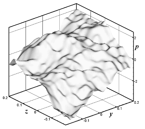
Figure 8: Relief of the kinematic SZ effect. The height $p$ of the point $(y,z,p)$ on the $p(y,z)$ surface (the height above the $(y,z)$ plane) is proportional to the fluctuation amplitude $\Delta T_{r}(y,z)/T_{r}$ (1.4).

Let us show that the following law holds for the kinematic SZ effect:

$$\langle|\Delta T_{r}(r_{\bot 2})-\Delta T_{r}(r_{\bot 1})|\rangle=[\Delta(\Delta T_{r})]_{\Delta l_{\bot}}\propto(\Delta p)_{\Delta l_{\bot}}\propto(\Delta l_{\bot})^{5/6},$$

where $\Delta l_{\bot}=|r_{\bot 2}-r_{\bot 1}|,\,$ $r_{\bot}=(y,z)$ is a two-dimensional vector in the plane of sky. We restrict our analysis to the case $N_{\rm mix}\sim 1$ presented in Figs. 1-5 and 7-10. Below, we give a brief derivation. Let us consider two adjacent parallel $x$ lines of sight separated by a distance $\Delta l_{\bot}$. The value of $(\Delta p)_{\Delta l_{\bot}}$ is equal to the difference between the momenta $p$ (1.5) on these lines of sight. Let us calculate this difference. The contributions of large eddies with a size $l_{\rm rot}\,$ $(l_{\rm rot}>\Delta l_{\bot})$ to the difference between integrals (1.5) are small, because these contributions are almost equal on adjacent lines of sight. The contribution of small eddies $(l_{\rm rot}<\Delta l_{\bot})$ increases with size $l_{\rm rot}$ and reaches a maximum at $(l_{\rm rot}\sim\Delta l_{\bot})$. Consequently, eddies with sizes on the order of the separation between the lines of sight should be considered to estimate (1.8).

These eddies are uncorrelated. Indeed, the correlation in the velocity field induced by them decays on a scale $\sim\Delta l_{\bot}$. Therefore, the corresponding contribution to the difference $\Delta(\Delta T_{r})\propto\Delta p$ is accumulated through a random addition. According to formulas (1.5) and (1.7), the momentum from a single eddy is

$$\sim u_{\rm rms}\,(\Delta l_{\bot}/L_{\rm mix})^{-1/3}\,(\Delta l_{\bot}/L)/u_{\rm rms}.$$

There are $\sim L/\Delta l_{\bot}$ such eddies on a line of sight which has a length $\sim L\sim L_{\rm mix}$. Expression (1.8) follows from this and from the fact that the effect is proportional to the square root of number of small-scale eddies under consideration, because

$$(\Delta p)_{\Delta l_{\bot}}\sim(\Delta l_{\bot}/L_{\rm mix})^{-1/3}\,(\Delta l_{\bot}/L)\,\sqrt{L/\Delta l_{\bot}}.$$

Scaling (1.8) is valid in the Kolmogorov range of scales $L_{\nu}<\Delta l_{\bot}<L_{\rm mix}$. In observations of $\Delta T_{r}/T_{r}\propto p$ or in direct numerical simulations, the small-scale limit is determined by the aperture resolution or the spatial mesh step, respectively.

1.3 Comparison of the Two Methods for Studying Turbulence

Let us compare the two effects under discussion, the Doppler broadening of X-ray lines and the kinematic SZ effect. The map of CMB intensity (1.4) carries information about the momentum of a unit column along the line of sight. This gives the velocity relative to the frame of reference associated with the CMB near the cluster, i.e. its peculiar velocity. The X-ray line profiles are more informative. In the simplest case of an isothermal plasma with a constant iron abundance, they provide information about the velocity distribution of matter relative to the velocity of the cluster as a whole (in particular, the velocity dispersion). Below, we discuss in detail several characteristic features of the spectrum and their relationship to the turbulent velocity field.

To compare the two effects, Fig. 9 shows a map of the velocity distributions $f_{H}(\Delta E)$ over the $(y,z)$ cluster plane. The distributions $f_{H}(\Delta E)$ were computed at the points located at the center, vertices, and middles of the sides of the $2l\times 2l$ square shown in Figs. 7 and 8. We took a frame of reference in which the total momentum $\int\int p(y,z)dydz$ of the emitting and scattering matter is equal to zero. We are looking for the distributions $f_{H}(\hat{u})$ in this frame. The scale of dimensionless velocities $\hat{u}$ was recalculated to energy shifts $\Delta E$ by using formula (1.3) at $u_{\rm rms}=270$ km s^-1. The velocity dispersion changes from point to point in the plane of the sky, $u_{\rm rms}=u_{\rm rms}(y,z)$. For definiteness, in the normalization $u_{\rm rms}=270$ km s^-1, we chose the dispersion at the center $y=0,z=0$. Note that the dispersion over the cluster as a whole appreciably exceeds the local dispersion. The relief of the kinematic SZ effect is determined by the shift velocity distribution (average velocity of the column as a whole). We see from Figs. 2 and 5 that these shift velocities give a large contribution to the velocity dispersion in the cluster as a whole.

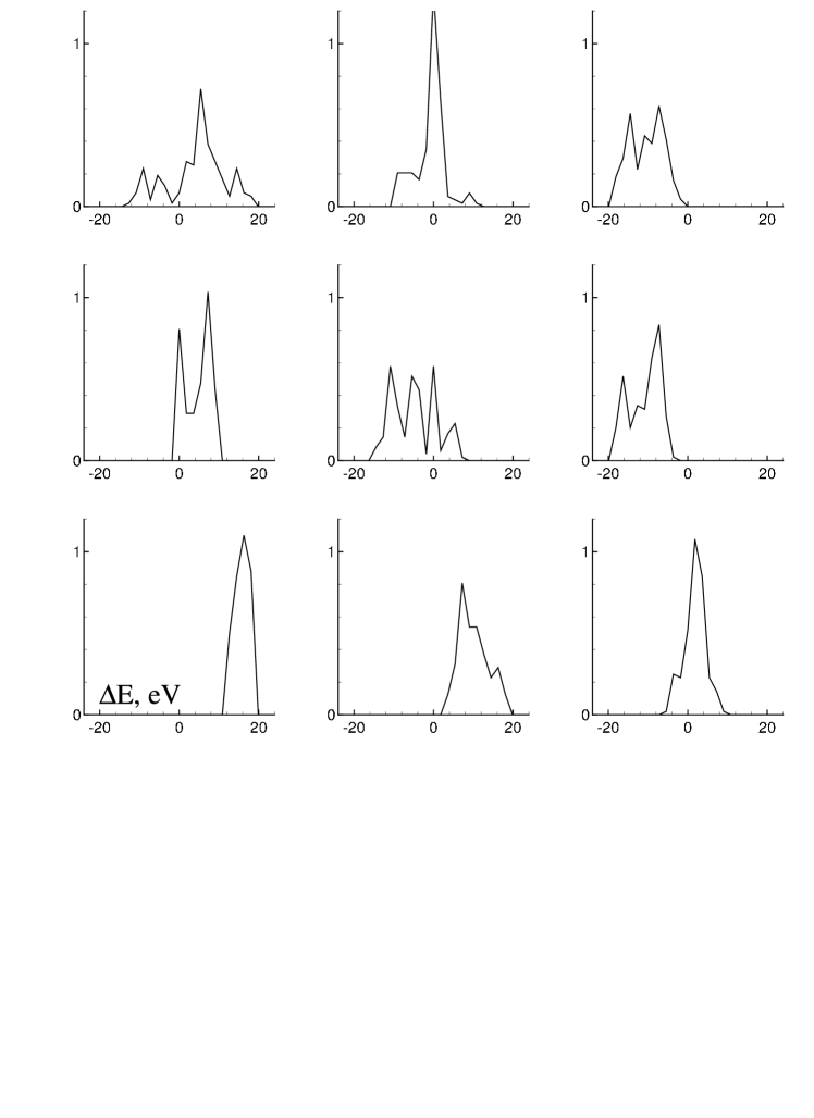
Figure 9: A map of the $f_{H}(\Delta E,y,z)$ profiles for iron ions in the $(y,z)$ plane at the points that coincide with the center, vertices, and middles of the sides of the square shown in Fig. 7 (a).

The $f_{\rm HT}(\Delta E)$ profiles of Fe XXV $(E_{0}=6.7keV)$ lines with turbulent and thermal broadenings are drawn in Fig. 10. They were obtained from the distributions $f_{H}(\Delta E)$ in Fig. 9 by folding with the Maxwellian distribution at $kT=3$ keV. Thermal smoothing “blurs” some of the features in the hydrodynamic distribution $f_{H}$, although the spectra remain fairly complex and varied. The centers of the $f_{H}(\Delta E)$ and $f_{\rm HT}(\Delta E)$ profiles coincide. Of course, they coincide with the profile center determined from the line-of-sight momentum $p(y,z)$. Therefore, the map of the kinematic SZ effect (Figs. 7 and 8) is simultaneously the map of the shifts in the profile centers in Figs. 9 and 10. Let us show this by using an example. The black color in the left panel of Fig. 7 (a) (the lower left corner of the square) corresponds to high velocities directed toward the observer. These velocities clearly show up in the rightward shift of the profile along the energy axis from $\Delta E=0$ in the spectrum in the lower left corner of Figs. 9 and 10, because motion toward the observer causes the photon energy to change. The shifts of the profile center as the position varies in the plane of the sky are large (3-6 local velocity dispersions). Thus, it is possible to independently and experimentally determine the shifts of the profile center by two different methods (the kinematic SZ effect and analysis of the line profile).

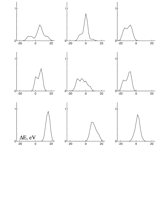
Figure 10: The $f_{\rm HT}(\Delta E)$ profiles of Fe XXV lines at $kT$ = 3 keV (the same as Fig. 2 but in linear coordinates). The spectrum shown in the middle panel of the upper row from the three panels was used to construct Figs. 1 and 4 (a). The central and bottom left panels were used in Figs. 4 (b) and (c).

The line shape completely changes during the shift to a large distance $\Delta l_{\perp}\sim L$ in a direction transverse to the $x$ line of sight $(N_{\rm mix}\sim 1)$. The shape changes continuously: the change in shape is small for small shifts. For example, the variation of such a parameter as the shift of the profile center during transverse shifts is shown in Fig. 7 (c). The profiles significantly deviate from the Gaussian profiles (a large shift of the spectrum center, splitting of the maximum, a sharp break in the exponential tails). A comparison with the Gaussian distribution for the middle spectrum from the upper triplet of spectra (Figs. 2 and 10) is shown in Fig. 1.

The presence of turbulence in the intergalactic cluster gas and its amplitude can also be judged from differences in the intensity distributions of permitted from one side and forbidden, intercombination lines and their satellites from another side over the cluster (Gilfanov et al. 1987). The optical depth in permitted lines can appreciably exceed unity in the absence of turbulence. Turbulent broadening reduces the optical depth in lines and this effect. This is a third independent method for studying turbulence in clusters of galaxies (Churazov et al., 2003).

Note that Fabian et al. (2003) pointed to the existence of long cold $H_{\alpha}$-emitting filaments in the Perseus cluster of galaxies as an argument against the well-developed turbulence in this cluster.

The full paper is arranged as follows. Section 2 gives a geometrical formulation of the problem with projection onto the observer’s direction (line of sight). Section 3 presents three main components of the Kolmogorov model: two boundaries with the sizes $(L_{\rm mix},$ $L_{\nu})$ of the inertial hierarchy of eddies and fluctuation amplitude scaling. Section 4 is devoted to the Fourier expansion with random phases of the turbulent velocity field. The procedure for calculating the velocity distribution $f_{H}(u)$ from the specific realization $u(x)$ of a random velocity field is described in Section 5. The distribution $f_{H}(u)$ can be approximately calculated from the first moments of the turbulent velocity field (Section 6). When there are many mixers, $N_{\rm mix}\gg 1,$ the turbulent distribution $f_{H}(u)$ tends to a Gaussian distribution $f^{G}(u)$ (Section 7). The superposition of thermal and hydrodynamic broadenings is analyzed in Section 8. A theory of the turbulent profile shape is constructed in Sections 9 and 10. We elucidate the question of typical spikes in the profile and its wings and the variety of possible shapes. The transverse correlations (in the plane of the sky) are studied in Section 11. The Lorentz line broadening is taken into account in Sections 12 and 13.

2 Turbulence and Doppler Shift

We are interested in the emission from the hot intergalactic plasma that fills cluster of galaxies. The plasma is in hydrostatic equilibrium in the gravitational well produced by collision-less dark matter. The density decreases toward the periphery of the well on scales of the order of the cluster scale L. The kinetic energy of the turbulent motion caused by mergers reaches $\sim 15\%$ of the thermal energy. By the meaning of the formulated problem (Doppler shift), the hydrodynamic density and plasma temperature fluctuations, which affect the local intensity but not the frequency, are of little importance. The velocity fluctuations are dominant.

There is a three-dimensional velocity field $\vec{v}(\vec{r},t)$. It is necessary to determine the Doppler shift in a frame of reference in which the cluster as a whole is at rest. We will consider the line profile when the X-ray telescope is pointed at a point in the cluster plane of the sky. The profile is defined by the function $u(x,t)$ that specifies the velocity $u$ along the $x$ line of sight passing through the observer and the point at which the telescope is pointed. The small eddies that are localized at the points separated along the $x$ axis are statistically equivalent. The turnover time of large-scale eddies is much longer than the time it takes for light to pass through the cluster. In addition, the evolution time of even the smallest observed velocity fluctuations is much longer than the exposure time during which an object is observed from a satellite. Consequently, we may omit the time dependence of the function $u(x,t)$ and deal with the instantaneous velocity field $u(x)$.

The Doppler change in photon energy $\Delta E=E-E_{0}$ is

$$\Delta E/E_{0}=-u/c,\;\;\;\;\;\Delta E\,[\,{\rm eV}\,]=6.7\,(u/300\,[\,{\rm kms}^{-1}\,]\,)\,(E_{0}/6700\,[\,{\rm eV}\,]\,)$$

where $E_{0}$ is the energy of the photon emitted from a region that is at rest relative to the cluster as a whole, and E is the energy of the photon emerged from a region that moves with velocity $u$ relative to the adopted frame of reference. Let the cluster be to the right of the observer on the $x$ axis. Accordingly, the velocity $u$ is positive if the emitting region recedes from the observer.

3 The Kolmogorov Model

An individual line profile corresponds to each velocity field $u(x)$. We are interested in statistically representative realizations of $u(x)$. The Kolmogorov views of turbulence are of great importance in constructing a typical profile. The point is that they solve the difficult question regarding the contribution of small-scale fluctuations.

In a Kolmogorov cascade, energy is transferred from large to small scales. The largest eddies have scales on the order of the mixer size $L_{\rm mix}$. The size $L_{\nu}$ of the smallest eddies is determined by viscous dissipation. A cluster of volume $L^{3}$ is assumed to be covered by a three-dimensional mesh of $N^{3}_{\rm mix}$ statistically equivalent mixers,

$$N_{\rm mix}=L/L_{\rm mix}.$$

The $\vec{v}(\vec{r})$ fluctuations are isotropic in velocity vector orientation. The $x$ axis is not highlighted in any way. Therefore, the Kolmogorov scaling (1.7) can be written for the $x$ velocity component (the projection of three-dimensional fluctuations onto the line of sight). In the hierarchy of scales, the mean energy losses $\dot{E}$ within the inertial range are scale-independent (Kolmogorov 1941),

$$\dot{E}\sim[\,(\Delta u)_{\Delta t}\,]^{2}/\Delta t\sim[\,(\Delta u)_{\Delta x}\,]^{3}/\Delta x,$$

where $\dot{E}$ are the hydrodynamic energy losses per gram of matter, and $\Delta u$ is the velocity variation due to the shift in time $\Delta t$ or along the line of sight $\Delta x$. The Kolmogorov scaling follows from (3.2):

$$(\Delta u)_{\Delta x}\sim\dot{E}^{1/3}\,(\Delta x)^{1/3}.$$

The locally viscous dissipation is given by the formula

$$\dot{E}=(\nu/2)\sum\sum\,(\partial v_{i}/\partial x_{j}+\partial v_{j}/\partial x_{i})^{2}\sim\nu\,[\,(\Delta u)_{\nu}\,]^{2}/[\,(\Delta x)_{\nu}\,]^{2},$$

where $(\Delta u)_{\nu}$ and $(\Delta x)_{\nu}$ are, respectively, the velocity and diameter scales of eddies on which viscous dissipation takes place. To estimate these scales, law (3.3) is extended to the range of dissipation through viscosity (Kolmogorov 1941; Monin and Yanglom 1965; Landau and Lifshitz 1986). We then find from formula (3.4) that

$$(\Delta x)_{\nu}\sim\nu^{3/4}/\dot{E}^{1/4}\sim(c_{s}/u_{\rm rms})^{3/4}\,l_{p}^{3/4}\,L_{\rm mix}^{1/4},$$

$$N_{\nu}=L/(\Delta x)_{\nu},\;\;\;\;\;(\Delta t)_{\nu}\sim\sqrt{\nu/\dot{E}},$$

where $c_{s}$ is the speed of sound, $u_{\rm rms}$ is the characteristic hydrodynamic velocity (rms deviation or dispersion) defined by the second moment

$$(\,u_{\rm rms}\,)^{2}=\int u^{2}\,dx/L$$

of the function $u(x)$ (the integral is taken over a range on the order of $L$), and $l_{p}$ is the proton mean free path. Large-scale eddies mainly contribute to the dispersion $u_{\rm rms}$ and the kinetic energy of the turbulence. $N_{\nu}$ (3.5) gives the number of the smallest eddies on the characteristic cluster scale. Formulas (3.5) and (3.6) define the smallest scales.

The size of small eddies (3.5) is mainly determined by the proton mean free path $l_{p}$. The latter varies over a wide range (many orders of magnitude) with amplitude of the random magnetic field in the intergalactic plasma of the cluster. Below, we give the corresponding estimates. In the absence of a magnetic field, the plasma viscosity

$$\nu=0.48\,v_{\rm Tp}\,l_{p}=1.5\cdot 10^{27}\,(kT)^{5/2}/n_{-2},$$

$$l_{p}=v_{\rm Tp}\,\tau_{p}=7.2\cdot 10^{19}\,(kT)^{2}/n_{-2},\;\;\;\;v_{\rm Tp}=\sqrt{2kT/m_{p}}$$

is determined by Coulomb collisions between ions (see, e.g., Rosenbluth and Sagdeev 1983); in what follows, the kinematic viscosity $\nu$ and the mean free path $l_{p}$ are in CGS units, the temperature kT is in keV, $n=10^{-2}n_{-2}$ cm^-3, $m_{p}$ is the proton mass. The gyroviscosity of plasma with a magnetic field is given by the expression (Rosenbluth and Sagdeev 1983)

$$\nu=0.5\,kT/m_{p}\,\omega_{\rm cp}=0.25\,v_{\rm Tp}\,r_{L},\;\;\;\;\;r_{L}=m_{p}\,v_{\rm Tp}\,c/eH,$$

where $\omega_{\rm cp}$ is the cyclotron frequency of protons, and $r_{L}$ is their Larmor radius. The viscous scale ratio is

$$\frac{\Delta x_{\nu}(H=0)}{\Delta x_{\nu}(H\neq 0)}=(1.92\,\tau_{p}\,\omega_{\rm cp})^{3/4}=2.3\cdot 10^{6}\,(\,H_{-8}\,)^{3/4}\,(\,kT\,)^{9/8}\,(\,n_{-2}\,)^{-3/4},$$

where $H=10^{-8}H_{-8}$ G. Accordingly, the dimensionless viscous wave numbers $N_{\nu}$ (3.5) are

$$N_{\nu}(H=0)=900\,(\,N_{\rm mix}\,)^{1/4}\,\mathop{\rm Ma}\nolimits^{3/4}\,(\,L_{200}\,)^{3/4}\,(\,n_{-2}\,)^{3/4}\,(\,kT\,)^{-3/2},$$

$$N_{\nu}(H\neq 0)=3.5\cdot 10^{9}\,(\,N_{\rm mix}\,)^{1/4}\,\mathop{\rm Ma}\nolimits^{3/4}\,(\,L_{200}\,)^{3/4}\,(\,H_{-8}\,)^{3/4}\,(\,kT\,)^{-3/8},$$

where Ma = $u_{\rm rms}/c_{s};$ $u_{\rm rms}$ and $c_{s}$ are the characteristic hydrodynamic velocity and the speed of sound, respectively; and $L=200L_{200}$ kpc.

In a hot rarefied plasma without a magnetic field, the mean free path $l_{p}$ is very large. Thus, a situation where $N_{\nu}$ is very small $(N_{\nu}\sim 1)$ is hypothetically possible. As we show in Sections 9 and 10 of the full paper, the line profile in this situation exhibits features that allow it to be distinguished from the case with $N_{\nu}\gg 1$. Currently available estimates based on Faraday rotation measurements give magnetic field strengths in the range 1-10 $\mu$G (see, e.g., Ge and Owen 1993), suggesting that the Kolmogorov range in the intergalactic turbulence spectrum is very wide.

4 Fourier Expansion

For the line profile to be constructed, we must know the velocity distribution $f_{H}(u)$. The distribution $f_{H}(u)$ can be calculated from the velocity field $u(x)$. Let us write out an analytical formula for the function $u(x)$ that satisfies law (3.3). It would be natural to represent the stochastic turbulent motions in the Kolmogorov range of scales as a Fourier series

$$u^{\prime}(x;\vec{\psi})=(\,N_{\rm mix}\,)^{\alpha}\,{\rm Re}\sum_{n=N_{\rm mix}}^{N_{\nu}}n^{-\alpha-1/2}\,\exp(i\psi_{n})\,\exp\left(i2\pi nx/L\right).$$

In formula (4.1), the index $\alpha$ specifies the velocity fluctuation scaling $(\Delta u)_{\Delta x}\propto(\Delta x)^{\alpha}$. In case (3.3), $\alpha=1/3$. The phases $\vec{\psi}=\{\psi_{n}\}$ in the harmonic expansion (4.1) are independent random variables uniformly distributed in the segment [0,2$\pi$]. The velocity is given by the real part of expansion (4.1) (the symbol Re). The summation limits (4.1) coincide with boundaries (3.1) and (3.5) of the inertial range. The function of $x$ (4.1) is considered in the segment $[l_{1},l_{2}]$ with a length on the order of $L$. Series (4.1) describes the fractal curve $u(x)$ whose fluctuations satisfy the Kolmogorov scaling law (3.3). This series makes it possible to carry out specific calculations.

Let us “displace” the auxiliary function u’ (4.1) so that the velocity field is centered $(\int u_{0}\,d_{x}=0)$. We change $u^{\prime}\rightarrow u_{0}$, where

$$u_{0}(x)=u^{\prime}(x)-u_{1},\;\,u_{1}=\int_{l_{1}}^{l_{2}}u^{\prime}(x)\,dx/l_{21},\;\;l_{21}=l_{2}-l_{1},\;(l_{1},l_{2})\sim L,$$

the function $u^{\prime}$ is calculated from formula (4.1). We normalize the function $u_{0}$ (4.2) to the rms velocity $u_{\rm rms}$. By definition, $u_{rms}$ gives the dispersion $\sigma$ of the velocity distribution. The velocity dispersion, along with the kinetic energy of the turbulence, is determined by large eddies. We write

$$u(x)=u_{0}(x)/u_{\rm rms},\;\;\;\;u_{\rm rms}^{2}=\int_{l_{1}}^{l_{2}}[\,u_{0}(x)\,]^{2}\,dx/l_{21}.$$

Below, we deal with the centered (4.2) and normalized (4.3) function $u(x)$ defined by formulas (4.1)-(4.3). The model of a homogeneous cloud with size $L$ is used as the first approximation to the density distribution. Clearly, this picture can be easily generalized to the real density distribution in clusters of galaxies.

5 The Velocity Distribution

Let us explain the meaning of the distribution $f_{H}(u)$. There is a function $u(x)$. Let us divide the $u$ axis into segments $\delta u$ that are small compared to the viscous fluctuation amplitude $(\Delta u)_{\nu}$. Consider an arbitrary point $u_{\star}$ on the $u$ axis. By definition,

$$f_{H}(u_{\star})=dp/du=\sum\delta x/l_{21}\,\delta u,$$

where the differential $dp$ characterizes the “weight” of the set of subregions that move with velocity $u_{\star}$. We assume that the argument of the function $u(x)$ belongs to the region $l_{1}\leq x\leq l_{2}$ inside the cluster. The condition $u_{\star}-\delta u/2\leq u(x_{\star})\leq u_{\star}+\delta u/2$ is satisfied in each of the small segments $\delta x$ in sum (5.1). In this condition, the points $x_{\star}$ belong to any of the small segments $dx$ in sum (5.1). Because of the statistical pulsations in velocity $u(x)$, sum (5.1) can contain many terms. Their number is approximately equal to the numbers of intersections of the function $u=u(x)$ with the straight line $u=u_{\star}$. It is easy to see that distribution (5.1) is normalized, $\int_{-\infty}^{\infty}f_{H}\,du=1$. The corresponding illustration is presented in Fig. 11.

Let us first consider an example with a monotonic function $u(x)$ and then return to the non-monotonicity and multivaluedness of the function $x(u)$ that is the inverse of $u(x)$ and to the turning points. In the monotonic case,

$$1/[\,du(x)/dx\,]=dx(u)/du=l_{21}f_{H}(u);$$

i.e., the velocity gradient determines $f_{H}$. The equations $u=u(x)$ and $f_{H}=\left[l_{21}\frac{du(x)}{dx}\right]^{-1}$ parametrically specify the distribution $f_{H}(u)$. Eliminating the parameter $x$ from this pair of equations yields an explicit dependence $f_{H}(u)$.

Let $u(x)=U\sin(2\pi x/L)$. Eliminating the parameter $x,$ we then obtain

$$f_{H}(u)=\left(\,l_{21}\,du/dx\,\right)^{-1}=\frac{L}{2\pi l_{21}}\,\frac{1}{U\cos(2\pi x/L)}=\frac{L}{2\pi l_{21}}\,\frac{1}{\sqrt{U^{2}-u^{2}}}.$$

Expression (5.2) specifies the dependence $f_{H}(u)$ in explicit form. Of course, an explicit expression can be derived only for very simple functions $u(x)$.

The example with an oscillating function $u(x)$ clearly illustrates an interesting singularity of the distribution $f_{H}$ in the cold case. It becomes infinite at the stop, turning, or cuspidal points of the inverse function $x(u)$ that are the extrema of the function $u(x)$; because of the root behavior, the distribution $f_{H}(u)$ is asymmetric about the singularity. The case with one harmonic (5.2) is an example that greatly differs from the Gaussian distribution. In this example, the dependence $f_{H}(u)$ has a minimum at the center and a singular break in the distribution tail. Consequently, in this example, the regions in which there is motion relative to the observer are more representative than the regions at rest (that is why the distribution maximum is off the center). As we will see below, in the case of many harmonics, the turning points or extrema lead to a needle-shaped distribution $f_{H}(u)$.

Thus, it is clear that distribution (5.1) is, in a sense, obtained by “projecting” the inverse function $x(u)$ onto the $u$ axis, as shown in Fig. 11 (the connection between Figs. 11 (a) and (b)). Fig. 11 (a) shows a realization of $u(x)$ (4.1)-(4.3) with random phases $\psi_{n}\,$ $(N\leq n\leq N_{\nu},\,$ $N_{\rm mix}=2,N_{\nu}=100)$ in the interval $l_{1}\leq x\leq l_{2}\,$ $(l_{1}=0.2L,l_{2}=0.7L)$. The viscous limit is fairly close: $(\Delta x)_{\nu}=l_{21}/N_{\nu}\sim 10^{-2}L,\,$ $(\Delta u)_{\nu}\sim 0.1u_{\rm rms}$. The viscous values determine the heights and widths of the $u(x)$ spikes (Fig. 11).

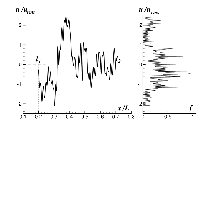
Figure 11: A scheme for recalculating the instantaneous velocity field $u(x)$ (a) to the velocity distribution $f_{H}(u)$ (b). The recalculation is performed by “projecting” the multi-valued function $x(u)$ (the inverse of the function $u(x)$) onto the $u$ axis. The $f_{H}(u)$ profile is similar to the profile of a hydrodynamically (without thermal broadening) broadened line.

In calculating the distribution $f_{H}(u)$, we substituted the velocity $u(x)$ with the set of its values $U_{i}$ at points $x_{i}=i\delta x$ (discretization). The $\delta x$ step was chosen to be small compared to the viscous length $(\Delta x)_{\nu}$ in order to resolve dissipating eddies. The distribution $f_{H}(u)$ was calculated numerically. It was replaced by a histogram (Fig. 11 (b)) with a small velocity step $\delta u\ll(\Delta u)_{\nu}$ in order not to lose any fluctuation. Because of the discretization, the above singularities of the distribution $f_{H}(u)$ are cut off at turning points. The height of the spikes in the distribution $f_{H}(u)$ is on the order of $\sqrt{(\Delta u)_{\nu}/\delta u},$; cf. (5.2). The value of $f(u_{\star})$ at the step

$$u_{\star}-\delta u/2\leq u\leq u_{\star}+\delta u/2$$

of the histogram is proportional to the number of discretization points $U_{i}$ at the limits $u_{\star}\pm\delta u/2$. After the normalization $\int f_{H}\,du=1$, we obtain the distribution $f_{H}$ shown in Fig. 11 (b).

It would be natural to analyze the deviations from the Gaussian distribution together with the calculation of moments, because the extent to which the distribution is non-Gaussian can be characterized by the deviations of moments from their Gaussian values.

6 The Method of Moments

Above, we described the procedure for an exact calculation of the distribution $f_{H}$ (the example in Fig. 11). Concurrently, it is instructive to describe the method for its analytical calculation. We approximate the distribution $f_{H}$ by a polynomial

$$f(u)=a_{0}+a_{1}u+a_{2}u^{2}+...=\sum_{j=0}^{n_{app}}a_{j}u^{j}.$$

The calculation procedure is based on the fact that the moments are determined by two independent methods. Let us calculate the moments $\mu_{n}$ directly from the velocity field $u(x)$ and the distribution $f_{H}(u)$. By definition,

$$\mu_{n}=\int_{l_{1}}^{l_{2}}[u(x)]^{n}\,dx/l_{21}=\int_{-\infty}^{\infty}u^{n}\,f(u)\,du.$$

The first three moments are known (do not depend on the phases $\psi_{n}$): $\mu_{0}=1$ (the normalization condition $\int f_{H}\,du=1$), $\mu_{1}=0$ (centering (4.2)), and $\mu_{2}=1$ (the choice of velocity unit (4.3)).

We truncate series (6.1) at the approximation order $n_{\rm app}$. Expansion (6.1) contains $n_{\rm app}$ + 1 unknown coefficients $a_{n}$. Let us set up a system of equations to determine them. The equations are $\mu_{n}^{u}=\mu_{n}^{f}$, where the expressions for $\mu_{n}^{u}$ and $\mu_{n}^{f}$ are calculated from $u$ and $f_{H}$, respectively (see (6.2)). Let us first calculate the missing moments $\mu_{3}^{u},\mu_{4}^{u},$, …, $\mu_{n-app}^{u}$ from the velocity $u(x)$. For a given realization, these are just some specific numbers. We then express integrals (6.2),

$$\mu_{n}^{f}=\int_{u_{l}}^{u_{r}}u^{n}\,f(u)\,du,$$

in terms of expansion (6.1).

Moments (6.3) are linear forms in unknowns $a_{n}$. The coefficients of the forms depend on the left, $u_{l}<0$, and right, $u_{r}>0$, integration limits in (6.3). Clearly, the power-law approximation (6.1) does not describe the decaying tails of the distribution $f_{H}$. Polynomial (6.1) intersects the $u$ axis at points $u_{l}$ and $u_{r}$. Inside the segment $u_{l}\leq u\leq u_{r}$, the polynomial is positive.

Solving the linear system of equations $\mu_{n}^{u}=\mu_{n}^{f}$ for the unknowns $a_{n}$, we express $a_{n}$ in terms of the zeros $u_{l}$ and $u_{r}$ of the polynomial $f_{H}$ in the form of a rational function of $u_{l}$ and $u_{r}$. Substituting the derived expressions for $a_{n}(u_{l},u_{r})$ into (6.1) yields the distribution $f_{H}(u_{l},u_{r};u)$. The zeros $u_{l}$ and $u_{r}$ are defined by a system of two equations $f_{H}(u_{l},u_{r};u_{l})$ = 0 and $f_{H}(u_{l},u_{r};u_{r})$ = 0. At $n_{\rm app}$ = 2 (approximation (6.1) is a parabola), $u_{l}=-\sqrt{5}$ and $u_{r}=\sqrt{5}$. In high orders, the equations rapidly become cumbersome.

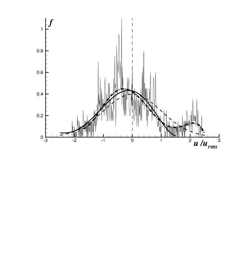
Figure 12: Comparison of the distributions $f_{H}(u):$ the thin fluctuating solid curve – exact calculation, the thick smooth solid curve – calculation by the methods of moments (a polynomial up to $u^{5}$ inclusive), the thick dot-dashed curve – a polynomial up to $u^{6},$ the thin dashed curve – Gaussian distribution $f^{G}.$ The distribution $f^{G}$ is symmetric about the vertical line $u=0.$

Examples of polynomials for $n_{\rm app}$ = 5 and 6 are given in Fig. 12. They refer to the realization of $u(x)$ shown in Fig. 11. The polynomials satisfactorily fit the exact distribution $f_{H}$. The sixth-order polynomial (heavy dash-dotted line) catches even the additional peak in the right wing. Of course, polynomials of a limited order smooth out the “needles” of the exact distribution. The Gaussian distribution is indicated in Fig. 12 by the dashed curve. We see the essentially non-Gaussian behavior, which manifest itself in the profile asymmetry relative to the dashed $u=0$ vertical line (Fig. 12) and in the break of the distribution tails and the appearance of additional peaks. In addition, the odd moments are nonzero, and the ratios of sequential even moments differ markedly from the Gaussian ratios. For the typical realization shown in Fig. 11, $\mu_{3}$ = 0.51 and $\mu_{5}$ = 2.97. The measure of smallness of the odd moments is determined by the normalization $\mu_{2}$ = 1 (4.3). The increase in the absolute value of the moment with increasing moment number should also be taken into account. In the Gaussian case, the following relations hold: $\mu_{4}^{G}=3\,(\mu_{2}^{G})^{2},$ $\mu_{6}^{G}=15\,(\mu_{2}^{G})^{3}$. In our case, however, $\mu_{4}/3=0.93$ and $\mu_{6}/15=0.71$.

Let us consider the influence of viscosity. To assess the role of the width of the inertial range log${}_{10}\frac{N_{\nu}}{N_{\rm mix}}$, we compared the velocities $u(x)$ and the distributions $f_{H}(u)$ with $N_{\nu}\sim 10^{2}$ and $N_{\nu}\sim 10^{3}$. As should be the case, the differences are attributable to the appearance of small-scale fluctuations as $N_{\nu}$ (3.5) greatly increases. The positions and shapes of the significant fluctuations with $\Delta_{u}\sim 0.1u_{\rm rms}$ depend weakly on $N_{\nu}$ if $N_{\nu}>100$. The first moments (up to the sixth moment inclusive) change only slightly (by $\sim$ 1%).

7 Gaussian Asymptotics

The main regulator on which the deviation of $f_{H}$ from the Gaussian distribution $f^{G}$ depends is the parameter $N_{\rm mix}$ that specifies the extent to which the scale of turbulence (3.1) is large. The viscous scale in this ratio is unimportant. Therefore, we set $N_{\nu}=\infty$. The difference between the distributions $f_{H}$ and $f^{G}$ decreases with increasing $N_{\rm mix}$. At $N_{\rm mix}=\infty$, the profile is Gaussian. Let us first show this and then present the results that illustrate the pattern of convergence $f_{H}\rightarrow f^{G}$ with increasing $N_{\rm mix}$.

Let us analyze the case with $N_{\rm mix}\gg 1$. Above, the calculations were associated with the dependence of velocity $u$ on coordinate $x$. In this case, the phases $\psi_{n}$ (4.1) were fixed. This is an approach with averaging over the coordinate. Let us look at the question differently. Let $x$ be fixed ($x=x_{\rm fix}$). The quantity $u(x_{\rm fix};\psi)=u(\psi)$ gives the velocity at point $x_{\rm fix}$ for a given set of phases $\psi$ (4.1). Let us study the statistics of $u(\psi)$ (an approach with phase averaging).

Since the phases $\psi_{n}$ are independent and random and the position $x$ is fixed, we may omit the regular oscillating factors exp ($i2\pi nx/L$) in (4.1). Consequently, the velocity $u(x_{\rm fix};\psi)$ is given by

$$u=(\,N_{\rm mix}\,)^{1/3}\sum_{n=N_{\rm mix}}^{\infty}\xi_{n}/n^{5/6},$$

where, in place of the phases $\psi_{n}$ we introduced the equivalent independent random variables $\xi_{n}\,$ $\langle\xi_{n}\rangle=0,$ and $\langle\xi_{n}^{2}\rangle=1$; $\,\langle\rangle$ denotes averaging. We assume, for simplicity, that $\psi_{n}$ takes on values of +1 or -1 with equal probabilities. The probability distribution function $f_{H}(u)$ of the random variable $u$ (7.1) should be determined.

We see from definition (7.1) that the mean velocity $\langle u\rangle$ is equal to zero. The probability distribution $f_{H}(u)$ is symmetric ($f_{H}$ is an even function of $u$). All odd moments are zero. It is easy to show that the second moment of (7.1) is

$$\langle u^{2}\rangle=(\,N_{\rm mix}\,)^{2/3}\sum_{n=N_{\rm mix}}^{\infty}n^{-5/3}=(\,N_{\rm mix}\,)^{2/3}\,\zeta(5/3,N_{\rm mix}),$$

where $\zeta$(5/3, $N_{\rm mix}$) is the generalized Riemann zeta function (Vinogradov 1979). In the limit $N_{\rm mix}\gg 1$, $\,\langle u^{2}\rangle=3/2$, because $\sum n^{-5/3}\approx\int dn/n^{5/3}$.

Let us calculate the fourth moment. We have

$$u^{4}/(\,N_{\rm mix}\,)^{4/3}=(\,\sum\xi_{n}/n^{5/6}\,)^{4}=-2\sum\xi_{n}^{4}/n^{10/3}+3\,(\,\sum\xi_{n}^{2}/n^{5/3}\,)^{2}+A.$$

In (7.3), the term $A$ is the sum of the terms with an odd number of factors $\xi_{n}$. After averaging, the term $A$ vanishes, and we obtain

$$\langle u^{4}\rangle/(\,N_{\rm mix}\,)^{4/3}=-2\sum n^{-10/3}+3\,(\,\sum n^{-5/3}\,)^{2}=-2\,\zeta(10/3,N_{\rm mix})+3\,[\,\zeta(5/3,N_{\rm mix})\,]^{2},$$

because $\xi_{n}=\pm 1$ and $\xi_{n}^{4}=1$. For $N_{\rm mix}\gg 1$, expression (7.4) tends to the limit

$$\langle u^{4}\rangle=3\,(3/2)^{2}.$$

As we see, the ratio of the fourth moment (7.5) to the square of the second moment (7.2), $\langle u^{4}\rangle/(\,\langle u^{2}\rangle\,)^{2}$, is equal to three. This should be the case for the Gaussian distribution. The aforesaid is also true for the random variables $\xi_{n}$ of a more general form than $\xi_{n}=\pm 1$. Indeed, for $N_{\rm mix}\gg 1$, sum (7.1) includes many approximately equal (in absolute value) independent random terms. In this case, in view of the central limit theorem, the probability distribution of the random variable $u$ is Gaussian. At $N_{\rm mix}\sim 1$, this is not the case, because th first terms in sum (7.1) significantly differ due to the factor $n^{-5/6}$.

Table 2.

$N_{mix}$	$\mu_{2}-1$	$\mu_{3}$	$R_{4}-1$	$R_{4}^{\zeta}-1$	$\mu_{5}$	$R_{6}-1$
$2\;(\star)$	$0$	$0.51$	$-0.07$		$2.97$	$-0.29$
$2$	$0$	$0.31$	$-0.11$	$-0.078$	$4.8$	$-0.21$
$10$	$0$	$0.21$	$-0.077$	$-0.013$	$1.7$	$-0.23$
$50$	$0$	$0.014$	$-0.045$	$-0.0026$	$0.25$	$-0.16$
$\infty$	$0$	$0$	$0$	$0$	$0$	$0$

It remains to study the convergence $f_{H}\rightarrow F^{G}$ with increasing $N_{\rm mix}$. The corresponding results are presented in Table 2.

This table shows how the moments converge to their Gaussian values (the last row). The moments $\mu_{n}$ are defined by formulas (6.2), $R_{4}=\mu_{4}/3\mu^{2}_{2},$ $\,R_{6}=\mu_{6}/15\mu_{2}^{3}$. The first moment is equal to zero due to centering (4.2). Because of normalization (4.3), the second moment is always equal to unity. In the Gaussian limit, $\mu_{3}=\mu_{5}=0$ and $R_{4}=R_{6}=1$. The procedure for calculating the moments $\mu_{3}-\mu_{6}$ was described in Section 5 and 6. The table list the mean values obtained by averaging over many realizations $\vec{\xi},u(x)$ (4.1). For the odd moments, we average the absolute value of the moment to establish the degree of deviation from zero. The realization-averaged values are given in rows 3-5 of Table 2. For comparison with a unit realization, the second row gives the values that refer to the example in Fig. 11; see also the end of Section 6. This row is highlighted by the symbol ($\star$). The formula

$$R_{4}^{\zeta}(N_{\rm mix})-1=\langle u^{4}\rangle/3(\,\langle u^{2}\rangle\,)^{2}-1=(-2/3)\,\zeta(10/3,N_{\rm mix})/[\,\zeta(5/3,N_{\rm mix})\,]^{2},$$

used in column 5 of the table follows from expressions (7.2) and (7.4). It shows the deviation from the Gaussian distribution in the case of averaging over all realization $\xi_{n}$. The corresponding $R_{4}$ calculated form the zeta function is denoted by the superscript $\zeta$.

Let us discuss the data in the Table 2. We see that the moments approach their Gaussian values as $N_{\rm mix}$ increases (refinement of the leading or dominant turbulence scale (3.1)). Therefor, the distribution $f_{H}$ also tends to $f^{G}$. As should be the case, the convergence in lower moments ($\mu_{3},\mu_{4}$) is faster than the convergence in higher moments ($\mu_{5},\mu_{6}$). The deviations in higher moments are larger, and they decrease with increasing $N_{\rm mix}$ more slowly. The main conclusion is that for large-scale turbulence with $N_{\rm mix}=2-10$ $\,(L_{\rm mix}\sim L$, (3.1)), there are significant deviations from the Gaussian distribution.

References

E. Churazov, M. Brüggen, C.R. Kaiser, et al. Astrophys. J. 554, 262 (2002a).

E. Churazov, R. Sunyaev, W. Forman, and H. Boehringer, Mon. Not. R. Astron. Soc. 332, 729 (2002b).

E. Churazov, W. Forman, C. Jones, R. Sunyaev, and H. Boehringer, Mon. Not. R. Astron. Soc. (2003 accepted); astro-ph/0309427.

A.C. Fabian, J.S. Sanders, C.S. Crawford, C.J. Conselice, J.S. Gallagher, and R.F.G. Wyse, Mon. Not. R. Astron. Soc. 344, L48 (2003).

C.S. Frenk, S.D.M. White, P. Bode, et al. Astronphys. J. 525, 554 (1999).

J.P. Ge and F.N. Owen, Astron. J. 105, 778 (1993).

M. R. Gilfanov, R.A. Sunyaev and E.M. Churazov, Sov. Astron. Lett 13, 3 (1987).

V.V. Ivanov, Radiative Transfer and the Spectra of Celestial Bodies, Nat. Bureau of Standards Spec. Publ. No. 385 (1973).

R.K. Janev, L.P. Presnyakov, and V.P. Shevelko, Physics of Highly Charged Ions. Springer Series in Electrophysics (Berlin: Springer, 1985), Vol. 13.

A.N. Kolmogorov, Dokl. Akad. Nauk SSSR 30, 299 (1941).

L.D. Landau and E.M. Lifshitz, Hydrodynamics (Nauka, Moscow, 1986) [in Russian].

Mathematical Encyclopaedia, Ed. by I.M. Vinogradov (Sov. Encyclopedia, Moscow, 1979), Vol. 2 [in Russian].

A. S. Monin and A.M. Yaglom Statistical Hydromechanics ( Nauka, Moscow, 1965) [in Russian].

D. Nagai, A. Kravtsov, and A. Kosowsky, Astrophys. J. 587, 524 (2003)/

M.L. Norman and G.L. Bryan, The Radio Galaxy Messier 87, Ed. by H.-J. Roeser and K. Meisenheimer (Springer, Berlin, 1999), Lecture Not. Phys. 530, ISSN0075-8450.

F.S. Porter and K. Mitsuda (Astro-E2/XRS Collab.) American Astron. Soc. HEAD Meeting No. 35, No. 33.05 (2003).

M.N. Rosenbluth and R.Z. Sagdeev, Handbook of Plasma Physics (North-Holland, Amsterdam, 1983).

R.K. Smith, N.S. Brickhouse, D.A. Liedahl, and J.C. Raymond, Astrophys. J. 556 L91(2001).

R.A. Sunyaev, Astron. Lett. 3 268 (1977).

R.A. Sunyaev, M. Norman, and G. Brian, Astronomy Letters 29 783 (2003); astro-ph/0310041.

R.A. Sunyaev and Ya.B. Zeldovich, Astrophys. Space Sci. 7, 3 (1970).

R.A. Sunyaev and Ya.B. Zeldovich, Mon. Not. R. Astron. Soc. 190, 413 (1980).