Axion bremsstrahlung from collisions of global strings

Abstract

We calculate axion radiation emitted in the collision of two straight global strings. The strings are supposed to be in the unexcited ground state, to be inclined with respect to each other, and to move in parallel planes. Radiation arises when the point of minimal separation between the strings moves faster than light. This effect exhibits a typical Cerenkov nature. Surprisingly, it allows an alternative interpretation as bremsstrahlung under a collision of point charges in $2+1$ electrodynamics. This can be demonstrated by suitable world-sheet reparameterizations and dimensional reduction. Cosmological estimates show that our mechanism generates axion production comparable with that from the oscillating string loops and may lead to further restrictions on the axion window.

I Introduction

For more than twenty years the Peccei-Quinn axion PQ77 ; W78 ; Wi78 remains one of the most serious dark matter candidates. Its properties depend essentially on one unknown parameter, the vacuum expectation value ${f}$ marking the energy scale of the U(1) symmetry breaking. The axion acquires a small mass

$$m_{a}\simeq 6\,{\rm\mu eV}\,\frac{10^{12}{\rm GeV}}{{f}}$$ (1)

in the QCD phase transition. The quantity ${f}$ is a free parameter of the theory, but it is severely constrained both by the accelerator physics and the astrophysics, the upper bound from the combined data being several meV. The lower bound is of cosmological origin and follows from the requirement that axions produced during the cosmological evolution do not overclose the Universe AS83 . The cosmological axion production is mainly due to the axion radiation from global strings and domain walls. In view of still persisting theoretical uncertainty, the corresponding lower bound lies between several units and several tens of $\mu$eV, corresponding to the maximal value of ${f}$ between $10^{12}$ and $10^{11}$ GeV. (For recent review of the present theoretical status of the axion see Sr02 ; the current astrophysical status of this model is reviewed in Si02 , earlier reviews include Re ).

The axion string network EV81 ; Vi85 ; GHV90 ; ViSh94 ; HiKi95 ; BaSh97 ; BaSh98 ; K98 ; BaSh99 is formed at the temperature of the Peccei-Quinn phase transition ${f}$, and it is usually assumed that the reheating temperature is higher than ${f}$, otherwise the network would get diluted by the exponential expansion; this introduces more uncertainty into theoretical predictions. Strings are primarily produced as long straight segments with length of the order of the horizon size, and they initially move with substantial friction DS87 ; VI91 ; MaSh97 due to scattering on them of the cosmic plasma particles. At some temperature $T_{*}<{f}$ the scattering becomes negligible and the string network enters the scale-invariant regime HS91 ; Na97 ; YKY98 when strings form closed loops via interconnections and move almost freely with relativistic velocities AlTu ; Sh87 . The standard estimates of the axion radiation from global strings are based on the assumption that the main contribution comes from the oscillating string loops D85 ; GaVa ; DS89 ; DaQu90 ; Sa ; BS94 ; YKY98 ; HCS99 ; HaChSi01 . The amount of radiation is large enough and leaves a rather narrow window for possible values of ${f}$.

Here we would like to discuss one additional mechanism of axion radiation: the bremsstrahlung which can be produced in collisions of long strings. In fact, the number of collisions of long strings is at least not smaller than the number of string loops which are formed under some of these collisions (note that in our case passing of strings through each other is not assumed). Meanwhile, as far as we are aware, this mechanism was not explored so far in the axion physics context. It works as follows. Neglecting the boundary effects, let us assume that two infinite straight strings move in parallel planes, the two strings being generically inclined with respect to each other. Then the point of minimal separation between the strings, which marks the localization of the effective source of axion radiation, is allowed to move with any velocity, superluminal in particular. In this latter case one can expect Cerenkov axion emission to emerge. Similar mechanism was earlier suggested for gravitational radiation of local strings GaGrLe93 , but in that case the explicit calculations have led to zero result. Vanishing of the gravitational radiation, however, has a specific origin related to the absence of gravitons in the $2+1$ gravity theory. Indeed, as it was explained in GaGrLe93 , two crossed superluminal strings can be “parallelized” by suitable coordinate transformations and world sheet reparameterizations, so the problem is essentially equivalent to the point particles’ collision in $2+1$ gravity theory. For other fields, (e.g. electromagnetic) this mechanism does work; see GGL for calculation of the Cerenkov electromagnetic radiation generated in collisions of superconducting strings. So one can expect to have a non-vanishing axion bremsstrahlung from collisions of global strings as well.

Our calculation follows the approach of GaGrLe93 and it is essentially perturbative in terms of the string-axion field interaction constant (equal to ${f}$) involving two subsequent iterations in the strings equations of motion and the axion field equations. This is similar to calculation of the bremsstrahlung from charged ultrarelativistic particles. In this latter case the iteration sequence converges if the scattering angle is small. We assume the same condition to hold for the strings, though we do not enter here into a detailed investigation of the convergence problem. We would like to mention also a similar perturbative approach in terms of geodesic deviations KHC .

II General setting

Consider a pair of relativistic strings

$$x^{\mu}=x_{n}^{\mu}(\sigma^{a}),\;\;\mu=0,1,2,3,\;\;\sigma_{a}=(\tau,\sigma),\;\;a=0,1,$$

where $n=1,2$ is the index labelling the two strings. The 4-dimensional space-time is assumed to be flat and the signature is chosen as $+,---$ and $(+,-)$ for the string world-sheets. Strings interact via the axion field $B_{\mu\nu}$ as described by the action BaSh97

$$S=S_{st}+S_{B},$$ (2)

where the string term is

$$S_{st}=-\sum_{n=1,2}\int\Big{(}\frac{\mu_{n}^{0}}{2}\sqrt{-\gamma}\gamma^{ab}\partial_{a}x_{n}^{\mu}\partial_{b}x_{n}^{\nu}\eta_{\mu\nu}+2\pi f_{n}B_{\mu\nu}\epsilon^{ab}\partial_{a}x_{n}^{\mu}\partial_{b}x_{n}^{\nu}\Big{)}d^{2}\sigma_{n},$$ (3)

and the field action is

$$S_{B}=\frac{1}{6}\int\limits H_{\mu\nu\lambda}H^{\mu\nu\lambda}d^{4}x.$$ (4)

Here $\mu_{n}^{0}$ are the (bare) string tension parameters, ${f}_{n}$ are the corresponding coupling parameters (their $n$-labelling helps to control the perturbation expansions), the Levi-Cività symbol is chosen as $\epsilon^{01}=1,\;\gamma_{ab}$ is the metric on the world-sheets.

The totally antisymmetric axion field strength is defined as

$$H_{\mu\nu\lambda}=\partial_{\mu}B_{\nu\lambda}+\partial_{\nu}B_{\lambda\mu}+\partial_{\lambda}B_{\mu\nu}.$$ (5)

Variation of the action (2) over $x^{\mu}_{n}$ leads to the equations of motion for strings

$$\mu_{n}^{0}\partial_{a}(\sqrt{-\gamma}\gamma^{ab}\partial_{b}x^{\mu}_{n})=2\pi f_{n}H^{\mu}_{\alpha\beta}V_{n}^{\alpha\beta},$$ (6)

where

$$V_{n}^{\alpha\beta}=\epsilon^{ab}\partial_{a}x_{n}^{\alpha}\partial_{b}x_{n}^{\beta},$$ (7)

and $H^{\mu}_{\alpha\beta}$ is the total field strength due to both strings (no external field is assumed). The corresponding potential two-form is the sum

$$B^{\mu\nu}=B^{\mu\nu}_{1}+B^{\mu\nu}_{2},$$ (8)

of contributions $B^{\mu\nu}_{n}$ due to each string:

$$\square B_{n}^{\mu\nu}=4\pi J_{n}^{\mu\nu}.$$ (9)

Here the Lorentz gauge ${\partial}_{\lambda}B^{\nu\lambda}=0$ is assumed, the 4-dimensional D’Alembert operator is introduced as $\Box=-\eta^{\mu\nu}{\partial}_{\mu}{\partial}_{\nu}$, and the source term reads

$$J_{n}^{\mu\nu}=\frac{f_{n}}{2}\int\limits V_{n}^{\mu\nu}\,\delta^{4}(x-x_{n}(\sigma_{n}))\,d^{2}\sigma_{n}.$$ (10)

The self-action terms in the equations of motion (6) diverge both near the strings and at large distances, so two regularization parameters $\delta$ and $\Delta$ have to be introduced BaSh95 . These can be absorbed by classical renormalization of the string tension as follows

$$\mu=\mu_{0}+2\pi f^{2}\log(\Delta/\delta).$$ (11)

The ultraviolet cutoff length $\delta$ is of the order of string thickness $\delta\sim 1/f$, while the infrared cutoff distance $\Delta$ can be taken as the correlation length in the string network.

Assuming that such a renormalization is performed, we are left with the same equations of motion (6) with the physical tension parameters $\mu_{n}$ which contain only the mutual interaction terms on the right hand side. The constraint equations for each string read :

$$\partial_{a}x^{\mu}\partial_{b}x^{\nu}\eta_{\mu\nu}-\frac{1}{2}\gamma_{ab}\gamma^{cd}(\partial_{c}x^{\mu}\partial_{d}x^{\nu}\eta_{\mu\nu})=0.$$ (12)

Using the invariance of the action (3) under separate world-sheet reparameterizations

$$\sigma^{a}_{n}\;\to\;\overline{\sigma}^{a}_{n}(\sigma^{a}_{n})$$ (13)

and under Weyl rescaling of the metric $\gamma_{ab},$ one can fix the flat gauge

$$\gamma_{ab}=\eta_{ab},$$ (14)

so that the constraint equations simplify to

$$\dot{x}^{2}+x^{\prime 2}=0,\quad\dot{x}^{\mu}x^{\prime\nu}\eta_{\mu\nu}=0$$ (15)

for each string, where dots and primes denote the derivatives over $\tau$ and $\sigma$ as usual. In the gauge (14) the renormalized equations of motion read :

$$\mu_{n}\left({\partial}_{\tau}^{2}-{\partial}_{\sigma}^{2}\right)x^{\mu}_{n}=2\pi f_{n}H^{\mu\nu\lambda}_{n^{\prime}}V_{\nu\lambda}^{n^{\prime}},\quad n\neq n^{\prime},$$ (16)

where the field $H^{\mu\nu\lambda}_{n^{\prime}}$ corresponds to the contribution of the $n^{\prime}-$th string (no sum over $n^{\prime}$). It is worth noting that imposing flat world-sheet metric we still do not fix the gauge completely, since one is free to perform two-dimensional linear transformations preserving the Minkowski metric (14) on the world sheets.

The retarded solution to the wave equation can be presented in its standard form

$$B_{n}^{\mu\nu}=4\pi\int G^{ret}(x-x^{\prime})J_{n}^{\mu\nu}(x^{\prime})d^{4}x^{\prime},$$ (17)

where the Green’s function is

$$G^{\rm ret}(x-x^{\prime})=\frac{1}{(2\pi)^{4}}\int\frac{{\rm e}^{-iq(x-x^{\prime})}}{q^{2}+2i\epsilon q^{0}}d^{4}q,$$ (18)

with $\epsilon\rightarrow+0$. The advanced Green’s function is obtained by changing the sign of $\epsilon$.

The energy momentum tensor for the axion field reads

$$T^{\mu\nu}=\left(H^{\mu\alpha\beta}H^{\nu}_{\alpha\beta}\ -\ \frac{1}{6}H_{\alpha\beta\gamma}H^{\alpha\beta\gamma}g^{\mu\nu}\right).$$ (19)

To avoid complications with definition of the wave zone for infinite strings, it is convenient to compute the radiation reaction power using the divergence equation

$$\frac{\partial T^{\mu\nu}}{\partial x^{\nu}}=-4\pi H^{\mu\alpha\beta}J_{\alpha\beta},$$ (20)

where $H^{\mu\alpha\beta}$ should be taken as the half-difference of the retarded and advanced solution of the wave equation, $H_{\rm rad}^{\mu\alpha\beta}=(H_{\rm adv}^{\mu\alpha\beta}-H_{\rm adv}^{\mu\alpha\beta})/2$. The corresponding potential has then the following Fourier transform:

$$B^{\rm rad}_{\mu\nu}(k)=-4i\pi^{2}\frac{k^{0}}{|k^{0}|}J_{\mu\nu}(k)\delta(k^{2})\ ,$$ (21)

where the current

$$J_{\mu\nu}(k)=\int J_{\mu\nu}(x){\rm e}^{ikx}d^{4}x$$ (22)

is transverse

$$k^{\mu}J_{\mu\nu}(k)=0$$ (23)

and taken on the mass-shell $k^{2}=0$ of the massless axion. The radiative loss of the 4-momentum during the collision can be evaluated as

$$P^{\mu}\ =\ \int\partial_{\nu}T^{\mu\nu}d^{4}x=-4\pi\int H_{\rm rad}^{\mu\alpha\beta}J_{\alpha\beta}d^{4}x\ .$$ (24)

Substituting (21) into (24) we obtain

$$P^{\mu}\ =\ \frac{1}{\pi}\int k^{\mu}\frac{k^{0}}{|k^{0}|}|J_{\alpha\beta}(k)|^{2}\delta(k^{2})d^{4}k.$$ (25)

Alternatively, this quantity can be presented as a square of the polarization projection of the Fourier-transform of the current. Indeed, in three dimensions the axion field propagating along the wave vector ${\bf k},\;k^{\mu}=(\omega,{\bf k}),$ has a unique polarization state

$$e_{ij}=\frac{1}{\sqrt{2}}(e_{i}^{\theta}e_{j}^{\varphi}-e_{i}^{\varphi}e_{j}^{\theta}),\quad i,j=1,2,3,$$ (26)

where ${\bf e}^{\theta}$ and ${\bf e}^{\varphi}$ are two unit vectors orthogonal to ${\bf k}$ and to each other:

$${\bf e}^{\varphi}\cdot{\bf e}^{\theta}=0,\quad{\bf k}\cdot{\bf e}_{i}=0.$$ (27)

Using antisymmetry and transversality of the current (23) and the completeness condition

$$e_{i}^{\theta}e_{j}^{\theta}+e_{i}^{\varphi}e_{j}^{\varphi}=\delta_{ij}-k_{i}k_{j}/\omega^{2},$$ (28)

one finds

$$\Delta P^{\mu}=\frac{1}{\pi}\int k^{\mu}\frac{k^{0}}{|k^{0}|}|J^{ij}(k)e_{ij}|^{2}\delta(k^{2})d^{4}k.$$ (29)

Integrating over $k^{0}$, we finally obtain

$$\Delta P^{\mu}=\frac{1}{\pi}\int\frac{k^{\mu}}{|{\bf k}|}|J({\bf k})|^{2}d^{3}k,$$ (30)

where

$$J({\bf k})=J^{ij}(k)e_{ij}$$ (31)

with $k^{0}=|{\bf k}|$. In what follows we shall use the following explicit parameterization of three orthogonal vectors by spherical angles :

$${\bf k} = \omega[\sin\theta\cos\varphi,\,\,\sin\theta\sin\varphi,\,\,\cos\theta],$$

$${\bf e}^{\varphi} = [-\sin\varphi,\,\,\cos\varphi,\,\,0],$$ (32)

$${\bf e}^{\theta} = [\cos\theta\cos\varphi,\,\,\cos\theta\sin\varphi,\,\,-\sin\theta].$$

Our strategy consists in solving the system of equations (16, 17) iteratively, by expanding all functions in powers of the coupling constant ${f}$:

$$B^{\mu\nu} = \sum_{l=1}^{\infty}{{}_{l}B}^{\mu\nu},$$ (33)

$$J^{\mu\nu} = \sum_{l=0}^{\infty}{{}_{l}J}^{\mu\nu},$$ (34)

$$x^{\mu}(\sigma) = \sum_{l=0}^{\infty}{{}_{l}x^{\mu}}(\sigma).$$ (35)

Such expansions have to be performed separately for each string. In our notation, the zeroth-order approximations for the string embedding functions ${}_{0}x^{\mu}_{n}(\sigma)$ give zeroth-order source terms ${}_{0}J^{\mu\nu}_{n}$, which generate the first order fields ${}_{1}B^{\mu\nu}_{n}$ originating on each string. These quantities, when substituted to the string equations of motion (16), will generate the first order terms ${}_{1}x^{\mu}_{n}$, and so forth. Convergence of this expansion (with a formal parameter ${f}$ which has a dimension of an inverse length) is difficult to explore in general. This is likely to depend substantially on the choice of the zeroth-order solution of the string equations of motion. In this paper, the strings are assumed to be in the unexcited state in the zeroth order, that is they are straight and freely moving. In this case it can be expected that the power series solutions will give sensible results (at least in the lowest appropriate order when radiation appears) if the deviation angle of colliding strings due to their lowest order interaction is small. We shall come back to this condition later on.

III Collision kinematics

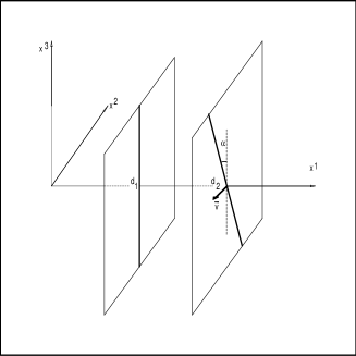
Figure 1: In the chosen frame, the first string is at rest, the second moves in the parallel plane separated from the first by an impact distance $d=d_{2}-d_{1}$ being inclined at the angle $\alpha$ with respect to the string at rest. Its velocity $v$ is perpendicular to the string itself.

The kinematics of collision is shown on Fig. 1. The unperturbed world-sheets of unexcited, freely moving straight (infinite) strings are described by linear functions of $\tau,\,\sigma$ :

$$_{0}x^{\mu}_{n}\ =\ d^{\mu}_{n}\ +\ u^{\mu}_{n}\tau_{n}\ +\Sigma^{\mu}_{n}\sigma_{n},\ \ \ n=1,2,$$ (36)

with $d^{\mu}_{n}$ and $\Sigma^{\mu}_{n}$ being space-like and $\ u^{\mu}_{n}$ time-like constant vectors. Then the constraint equations (15) imply the orthogonality and normalization conditions (choosing the unit norm time-like 4-velocity $u^{\mu}$ )

$$u^{\mu}\Sigma_{\mu}=0,\quad u^{\mu}u_{\mu}\ =1=-\Sigma^{\mu}\Sigma_{\mu}$$ (37)

for each string. We choose the reference frame such that the first string is at rest and is stretched along the $x^{3}$ axis:

$$u^{\mu}_{1}=[1,0,0,0],\quad\Sigma^{\mu}_{1}=[0,0,0,1].$$ (38)

The second string is assumed to move in the plane $x^{2},\,x^{3}$ with the velocity $v$ orthogonal to the string itself:

$$u^{\mu}_{2}=\gamma\,[1,0,-v\cos\alpha,v\sin\alpha],\quad\Sigma^{\mu}_{2}=[0,0,\sin\alpha,\cos\alpha],$$ (39)

where $\gamma=(1-v^{2})^{-1/2}$. We also choose both impact parameters $d^{\mu}_{n}$ to be orthogonal to $u^{\mu}$ and $\Sigma^{\mu}$ and aligned with the axis $x^{1}$, the distance between the planes being $d=d_{2}-d_{1}$. The angle of inclination $\alpha$ of the second string with respect to the first one can be presented in the Lorentz-invariant form as

$$\alpha=\arccos(-\Sigma_{1}\Sigma_{2}),$$ (40)

and the relative velocity of the strings as

$$v\ =\ (1-(u_{1}u_{2})^{-2})^{\frac{1}{2}}.$$ (41)

With this parametrization of the unperturbed world-sheets, the point of minimal separation between the strings (which always remains equal to $d$) moves with the velocity

$$v_{p}=\frac{v}{\sin\alpha}=(u_{1}u_{2})^{-1}\left(\frac{(u_{1}u_{2})^{2}-1}{1-(\Sigma_{1}\Sigma_{2})^{2}}\right)^{\frac{1}{2}}$$ (42)

along the $x^{3}$-axis. This motion is not associated with propagation of signal of any kind, so the velocity $v_{p}$ may be arbitrary, in particular, superluminal. The case of parallel strings corresponds to $v_{p}=\infty$.

Let us explore the residual gauge invariance consisting of the SO(1,1) transformations of the world-sheets

$$\tau_{n} \to \tau_{n}\cosh\chi_{n}+\sigma_{n}\sinh\chi_{n},$$

$$\sigma_{n} \to \tau_{n}\sinh\chi_{n}+\sigma\cosh\chi_{n},$$ (43)

preserving the constraints (15). It is easy to show that the relative orientation of two strings is not a gauge independent property GaGrLe93 . One can build the following matrix describing the relative orientation of the world-sheets

$$\kappa_{ab}=\partial_{a}x_{1}^{\mu}\partial_{b}x_{2}^{\nu}\eta_{\mu\nu},$$ (44)

whose determinant

$$\kappa=\det\kappa_{ab}=\gamma\cos\alpha$$ (45)

is invariant under the transformation (III). But the relative velocity (41) and the inclination angle (40) separately are not invariant. In particular, for superluminal strings one can always find the world-sheet boosts which make the strings parallel. This is achieved by the following choice of parameters in (III) for two strings

$$\tanh\chi_{1}=\frac{\sin\alpha}{v},\quad\tanh\chi_{2}=\frac{\tan\alpha}{\gamma v},$$ (46)

which exists if $v_{p}>1$. Note that strings are superluminal in the above sense provided that

$$\kappa=\gamma\cos\alpha\geq 1.$$ (47)

If this condition is not fulfilled, then the “parallelizing” transformation does not exist.

IV First order interaction

According to the conventions chosen above, the field equations (9) for the first order field terms ${}_{1}B^{\mu\nu}_{n}$ read :

$$\Box\,{{}_{1}B}_{n}^{\mu\nu}=4\pi\,{{}_{0}J}_{n}^{\mu\nu},$$ (48)

with the source terms (48)

$$_{0}{J^{\mu\nu}_{n}}=\frac{f_{n}}{2}\int\limits\,V_{n}^{\mu\nu}\delta^{4}\left(x-{{}_{0}x}_{n}(\sigma_{n})\right)\,d^{2}\sigma_{n},$$ (49)

where the zeroth-order quantities are found under the right-hand side integral :

$$V_{n}^{\mu\nu}=u_{n}^{\mu}\Sigma_{n}^{\nu}-\Sigma_{n}^{\mu}u_{n}^{\nu}.$$ (50)

In what follows we pass to the momentum representation according to the convention :

$$F(q)=\int F(x)\,{\rm e}^{iqx}\,d^{4}x,$$ (51)

where $qx=q_{\mu}x^{\mu}$. We will use similar notation for all scalar products, when there is no risk of ambiguity. The Fourier transform of the zeroth-order current (49) then reads :

$${}_{0}J^{\mu\nu}_{n}(q)=2\pi^{2}f_{n}{\rm e}^{iqd_{n}}\delta(qu_{n})\delta(q\Sigma_{n})V_{n}^{\mu\nu}.$$ (52)

The retarded solution ${{}_{1}B}^{\mu\nu}$ of the Eq. (48) generated by the zero-order source is

$$_{1}B_{n}^{\mu\nu}(q)=-\frac{8\pi^{3}f_{n}V^{\mu\nu}_{n}{\rm e}^{iqd_{n}}\delta(qu_{n})\delta(q\Sigma_{n})}{q^{2}+2i\epsilon q^{0}}.$$ (53)

Note that two $\delta$-functions in this expression shift the momentum $q$ from the pole $q^{2}=0$, so, as can be easily seen from the Eq. (25), the first order field is non-radiative.

The next step is to find corrections to the world-sheet embedding functions due to interaction between the strings via the axion field. Substituting (53) into the right hand side of the equations of motion (16) we obtain the following first-order perturbations of the string world-sheets

$$_{1}x_{1}^{\mu}=i\frac{2f_{1}f_{2}}{\mu_{1}}\int X^{\mu}_{1}\frac{\delta(qu_{2})\delta(q\Sigma_{2})\ {\rm e}^{iq(d_{2}-d_{1}-u_{1}\tau-\Sigma_{1}\sigma)}}{q^{2}[(q\Sigma_{1})^{2}-(qu_{1})^{2}]}d^{4}q,$$ (54)

where

$$X^{\mu}_{1} = q^{\mu}A+B_{1}\Sigma^{\mu}_{2}+C_{1}u_{2}^{\mu},\quad A=(u_{1}u_{2})(\Sigma_{1}\Sigma_{2})-(\Sigma_{1}u_{2})(u_{1}\Sigma_{2}),$$

$$B_{1} = (qu_{1})(u_{2}\Sigma_{1})-(\Sigma_{1}q)(u_{1}u_{2}),\quad C_{1}=(u_{1}\Sigma_{2})(\Sigma_{1}q)-(qu_{1})(\Sigma_{1}\Sigma_{2})\ .$$ (55)

Similarly for the second string

$$_{1}x_{2}^{\mu}=i\frac{2f_{1}f_{2}}{\mu_{2}}\int X^{\mu}_{2}\frac{\delta(qu_{1})\ \delta(q\Sigma_{1})e^{iq(d_{1}-d_{2}-u_{2}\tau-\Sigma_{2}\sigma)}}{q^{2}[(q\Sigma_{2})^{2}-(qu_{2})^{2}]}d^{4}q,$$ (56)

where

$$X^{\mu}_{2}=q^{\mu}A + B_{2}\Sigma^{\mu}_{1}+C_{2}u_{1}^{\mu},\quad B_{2}=(qu_{2})(u_{1}\Sigma_{2})-(\Sigma_{2}q)(u_{1}u_{2}),$$

$$C_{2} = (u_{2}\Sigma_{1})(\Sigma_{2}q)-(qu_{2})(\Sigma_{1}\Sigma_{2}),$$ (57)

with the same $A$. It can be checked that the quantities $X^{\mu}_{n}$ satisfy the conditions

$$X^{\mu}_{1}u_{1\mu}=X^{\mu}_{1}\Sigma_{1\mu}=X^{\mu}_{2}u_{2\mu}=X^{\mu}_{2}\Sigma_{2\mu}=0,$$ (58)

which ensure the fulfilment of the constraint equations (15) up to the first order.

To estimate the scattering angle $\delta\varphi$ of the string collision let us consider the case of parallel strings, $\alpha=0$. In the chosen frame one can use as an estimate for $\delta\varphi$ the ratio of the limiting value of the $x^{1}$ component of the 4-velocity of the second string and the initial $x^{2}$ component:

$$\delta\varphi\sim\lim_{\tau\to\infty}\frac{{}_{1}{\dot{x}}_{2}^{1}}{{}_{0}{\dot{x}}_{2}^{2}}.$$ (59)

To calculate the quantity in the numerator one has to integrate in (56) over $d^{4}q$. Integration over $q^{0}$ and $q^{3}$ is performed using delta-functions. Then, in the limit $\tau\to\infty$, an asymptotic relation

$$\lim_{\tau\to\infty}\frac{\sin[(qu_{2})\tau]}{qu_{2}}=\pi\delta(qu_{2})$$ (60)

gives one more delta-function, allowing integration over $q^{2}$. The last integration over $q^{1}$ reduces to

$$\int_{-\infty}^{\infty}\frac{{\rm e}^{iq^{1}d}dq^{1}}{q^{1}}=i\pi,$$ (61)

the resulting estimate for the scattering angle being

$$\delta\varphi\sim\frac{2\pi^{2}f^{2}}{\mu\,\gamma\,v^{2}},$$ (62)

where we have set $f_{1}=f_{2}$. Using the Eq. (11) for the renormalized string tension, in which we assume the second term to be dominant BaSh95 , we obtain

$$\delta\varphi\sim\frac{\pi}{\log{(\Delta/\delta)}\,\gamma\,v^{2}}\,.$$ (63)

The smallness of this quantity may serve as a rough estimate of the validity of the perturbation expansions (33-35). Therefore our iteration procedure works in the relativistic case $v\sim 1$, especially for ultrarelativistic collisions, $\gamma\gg 1$. But for global cosmological strings the quantity $\log{(\Delta/\delta)}$ is large enough. This improves the convergence of our iteration scheme even for $\gamma\sim 1$. Therefore our approach seems to be reasonably justified in realistic cosmological situations.

V Radiation

Using the first order corrections to the world-sheets of the string due to their lowest order interaction terms one can evaluate higher order terms of the expansion. Radiation emerges in the second approximation for the axion field ${}_{2}B^{\mu\nu}$ generated by the source term ${}_{1}J^{\mu\nu}$ which will be obtained from the first order contributions to the world-sheet embedding functions as follows:

$${{}_{1}J}^{\mu\nu}=\sum_{n=1,2}f_{n}\int\limits d^{2}\sigma\left[\left({{}_{0}\dot{x}}_{n}^{[\mu}{{}_{1}x^{\prime\nu]}_{n}}+{{}_{1}\dot{x}}_{n}^{[\mu}{{}_{0}x^{\prime\nu]}_{n}}\right)-\frac{1}{2}V_{n}^{\mu\nu}\,{{}_{1}x}_{n}^{\lambda}\,\partial_{\lambda}\right]\delta^{4}(x-{{}_{0}x}_{n}(\sigma_{n})),$$ (64)

where brackets denote anti-symmetrization over indices with the factor $1/2$. This follows from the fact that the Fourier-transform of this current is non-zero on the axion mass-shell $k^{2}=0$.

The Fourier transform of the first-order field source can be presented in the following form:

$$_{1}J^{\mu\nu}(k)=-8\pi^{2}f_{1}f_{2}\int\delta(qu_{2})\ \delta(q\Sigma_{2})\delta[(k-q)u_{1}]\ \delta[(k-q)\Sigma_{1}]{\rm e}^{i(d_{1}k)+q(d_{2}-d_{1}))}\left(\frac{f_{1}Q^{\mu\nu}_{1}}{\mu_{1}}\ +\ \frac{f_{2}Q^{\mu\nu}_{2}}{\mu_{2}}\right)\ ,$$ (65)

where the two terms

$$Q^{\mu\nu}_{1}\ =\frac{(q\Sigma_{1})u_{1}^{[\mu}{X_{1}^{\nu]}}-(qu_{1})\Sigma_{1}^{[\mu}{X_{1}^{\nu]}}-\frac{1}{2}V_{1}^{\mu\nu}(X_{1\lambda}k^{\lambda})}{q^{2}[(q\Sigma_{1})^{2}-(qu_{1})^{2}]}\ ,$$ (66)

$$Q^{\mu\nu}_{2}\ =\frac{[(k-q)\Sigma_{2}]u_{2}^{[\mu}{X_{2}^{\nu]}}-[(k-q)u_{2}]\Sigma_{2}^{[\mu}{X_{2}^{\nu]}}-\frac{1}{2}V_{2}^{\mu\nu}({X_{2\lambda}}k^{\lambda})}{(k-q)^{2}\{[(k-q)\Sigma_{2}]^{2}-[(k-q)u_{2}]^{2}\}}$$ (67)

could be associated with contributions of the first and the second string, respectively. It has to be noted, however, that in the second order the axion field is generated collectively by a source term containing symmetrically the contributions of the first order coming from both strings. It can be checked that the antisymmetric tensors $Q^{\mu\nu}_{n}$ satisfy the transversality conditions

$$k_{\mu}Q^{\mu\nu}_{1}=k_{\mu}{Q^{\mu\nu}_{2}}=0$$ (68)

ensuring in turn the transversality of the current ${}_{1}J^{\mu\nu}(k)$.

Integration over $q$-space is performed as follows. First, using $\delta[(k-q)u_{1}]$, we integrate over $q^{0}$, which fixes the value

$$q^{0}=k^{0}=\omega.$$ (69)

Then, using the delta-functions $\delta(qu_{2})$ and $\delta(q\Sigma_{2})$, one integrates over $q^{2}$ and $q^{3}$ obtaining

$$q^{2}=-\frac{\omega\cos\alpha}{v}\ ,\ \ q^{3}=\frac{\omega\sin\alpha}{v}.$$ (70)

The remaining delta-function $\delta[(k-q)\Sigma_{1}]$ does not further fix the vector $q^{\mu}$, but imposes an extra relation on the parameters :

$$k^{3}=\frac{\omega\sin\alpha}{v},$$ (71)

which is nothing but the Cerenkov condition for radiation emitted by an effective source moving with the velocity $v_{p}$ along the $x^{3}$ axis. Clearly, this motion is the motion of an effective source localized in the region surrounding the point of minimal separation between the strings where their deformation described by the first order interaction is maximal. This condition can be rewritten as the usual Cerenkov’s cone condition on the angle of emission

$$\cos\theta=1/v_{p},$$ (72)

which makes sense if $v_{p}\geq 1$. So the axion radiation is emitted inside the Cerenkov cone oriented along the $x^{3}$ axis (Fig. 2). In the limiting case $v_{p}=1$, radiation is emitted strictly along the $x^{3}$ direction; this occurs when the string inclination angle $\alpha$ is related to the string Lorentz factor as

$$\cos\alpha=\gamma^{-1},\,\ \,\ \ {\rm with}\,\ \ \,\ \,\ \,\gamma=(1-(u_{1}u_{2})^{-2})^{\frac{1}{2}}.$$ (73)

For $\cos\alpha<\gamma^{-1}$ no radiation is emitted at all. Therefore, string axion bremsstrahlung has essentially Cerenkov nature. But, rather surprisingly, it has another interpretation as a point charge bremsstrahlung in $2+1$ electrodynamics. We will come back to this in Sec. 7.

Integration over $q^{1}$ is performed using the contour integration in the complex plane. Denoting the impact parameter $d=d_{2}-d_{1}$ we obtain for the first term or (65)

$$\int\frac{{\rm e}^{-iq^{1}d}dq^{1}f_{1}(q^{1})}{(q^{1})^{2}+\kappa_{1}^{2}}=\frac{\pi f_{1}(-i\kappa_{1}){\rm e}^{-\kappa_{1}d}}{\kappa_{1}},$$ (74)

where $f_{1}$ stands for the remaining integrand, and

$$\kappa_{1}=\frac{\omega}{\gamma v}.$$ (75)

Similarly, the second term in (65) gives the integrals

$$\int\frac{e^{-iq^{1}d}dq^{1}f_{2}(q^{1})}{(k^{1}-q^{1})^{2}+\kappa_{2}^{2}}=\frac{\pi f_{2}(-i\kappa_{2})e^{-\kappa_{2}d+ik^{1}d}}{\kappa_{2}},$$ (76)

where

$$\kappa_{2}=\frac{\omega\xi}{v},\quad\xi=\cos\alpha+\frac{k^{2}}{\omega}v.$$ (77)

Therefore, the whole integral over $d^{4}q$ of the first term in (65) is proportional to the value of the integrand in the complex point $q^{\mu}={\bar{q}}^{\mu}$ where

$${\bar{q}}^{\mu}=\frac{\omega}{v}\,[v,\,-i/\gamma,\,-\cos\alpha,\,\sin\alpha],$$ (78)

with the corresponding value of $X_{1}^{\mu}$ being

$${\bar{X}}_{1}^{\mu}=\frac{\omega}{v}\,[0,\,i\cos\alpha,\,1/\gamma,\,0].$$ (79)

For the second term $Q_{2}^{\mu\nu}$ one finds instead the following quantities

$$k^{\mu}-{\bar{\;\bar{q}^{\mu}}}=\frac{\omega\xi}{v}\,[0,\,i,\,1,\,0],$$ (80)

$${\bar{\;\,\bar{X}_{2}^{\mu}}}=\frac{\gamma\omega\xi}{v}\,[v,\,-i\cos\alpha,\,-\cos\alpha,\,\sin\alpha].$$ (81)

Finally, projecting the current on the polarization tensor (26), we obtain the following lowest order approximation for the quantity (31):

$$_{1}J({\bf k})=\frac{4\sqrt{2}\pi^{3}f_{1}f_{2}}{\omega^{2}\gamma v\sin\theta}\delta(\cos\theta-1/v_{p})\cdot$$ (82)

$$\left(\frac{f_{1}{\rm e}^{-\omega d/v\gamma+ikd_{1}}}{\mu_{1}}(\cos\varphi-i\gamma\cos\alpha\sin\varphi)-\frac{f_{2}{\rm e}^{-\omega d\xi/v+ikd_{2}}}{\mu_{2}\gamma^{2}\xi^{2}}\left[\cos\varphi-i(v\xi\gamma^{2}\sin\theta+\sin\varphi)\right]\right),$$

where $\xi=\cos\alpha+v\sin\theta\sin\varphi$. Two terms here may be attributed to the contributions of the first (remaining at rest) and the second (moving) strings; in what follows we set $f_{1}=f_{2}=f,\,\mu_{1}=\mu_{2}=\mu$. The total amplitude is therefore a superposition of two terms exhibiting different frequency cutoff. The first term’s exponential factor leads to the isotropic condition

$$\omega\lesssim\frac{v\gamma}{d},$$ (83)

while the second gives a $\varphi-$dependent condition

$$\omega\lesssim\frac{v}{d\xi}=\frac{v}{d(\cos\alpha+v\sin\theta\sin\varphi)}.$$ (84)

In other words, the distribution of radiation on the Cerenkov cone is anisotropic. This feature becomes especially pronounced in the ultrarelativistic case.

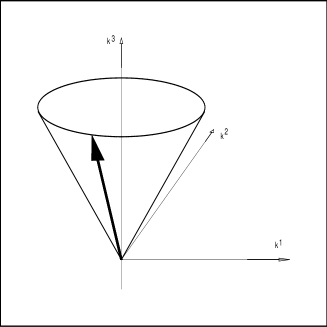
Figure 2: Radiation peaking on Cerenkov cone in the direction of motion of the relativistic sting.

Using the identity

$$\cos^{2}\alpha=v^{2}\sin^{2}\theta+\gamma^{-2}$$ (85)

which holds on the radiation cone, it is easy to show that when $\gamma\to\infty$, the quantity $\xi$ has a sharp minimum at $\varphi=-\pi/2$ corresponding to the direction of the moving string in the rest frame of the first string (see Fig. 2):

$$\xi\thickapprox\frac{1}{2\gamma^{2}\cos\alpha}\left(1+\beta^{2}\gamma^{2}\cos\alpha^{2}\right)],$$ (86)

where $\beta=\pi/2+\varphi\ll 1$. Due to the factor $\xi^{-2}$ in the second term in the amplitude (31), radiation is peaked in the direction $\varphi=-\pi/2$ within the narrow region

$$\beta\lesssim\gamma^{-1}.$$ (87)

The exponential factor exhibits similar peaking, provided

$$\gamma\cos\alpha\gg 1,$$ (88)

so the frequency range extends up to

$$\omega\lesssim\frac{\gamma^{2}}{d\,\cos\alpha}$$ (89)

in the angular region (87).

At the Cerenkov threshold

$$v=\sin\alpha,$$ (90)

the cone of emission shrinks $\theta\to 0$, in this case

$$\xi=\cos\alpha=\gamma^{-1}$$ (91)

and the amplitude (82) can be considerably simplified. Since in this limit $kd_{n}\to 0$, the oscillating factors $\exp{(ikd_{n})}$ become equal to unity, and one can check that the leading contributions of two terms in (82) cancel while $\theta\to 0$, that is the whole expression does not diverge. The remaining finite contribution reads

$$_{1}J({\bf k})=\frac{4i\sqrt{2}\pi^{3}f^{3}}{\mu\omega^{2}}{\rm e}^{-\omega d/v\gamma}\delta(\cos\theta-1).$$ (92)

Inserting this into the Eq. (30) and introducing the normalization length $l$ via the relation

$$\delta^{2}(\cos\theta-1)=\frac{l\omega}{2\pi}\delta(\cos\theta-1),$$ (93)

one obtains after integration over angles in $d^{3}k=\omega^{2}d\omega d\cos\theta d\varphi$ the total radiated energy per unit length of the string at rest

$$\frac{P^{0}}{l}=\int_{\Delta^{-1}}^{\infty}\frac{(2\pi)^{5}f^{6}}{\mu^{2}\omega}\exp({-2\frac{\omega d}{v\gamma}})d\omega,$$ (94)

where $\Delta$ is the frequency cutoff introduced in order to remove the infrared divergence of the spectral distribution of radiation. At the high frequency end the spectrum extends till the boundary (83). Integration over frequencies is performed in terms of the integral exponential function

$$\frac{P^{0}}{l}=\frac{(2\pi)^{5}f^{6}}{\mu^{2}}{\rm Ei}\left(1,\frac{2d}{v\gamma\Delta}\right).$$ (95)

For $d\ll v\gamma\Delta$,

$$\frac{P^{0}}{l}\approx\frac{(2\pi)^{5}f^{6}}{\mu^{2}}\ln\left(\frac{v\gamma\Delta}{2d{\rm e}^{C}}\right),$$ (96)

where $C$ is the Euler constant, ${\rm e}^{C}=1.781072418$. For $d\gg v\gamma\Delta$, one has

$${\rm Ei}\left(1,\frac{2d}{v\gamma\Delta}\right)\approx\frac{2d}{v\gamma\Delta}\exp\left(-\frac{2d}{v\gamma\Delta}\right),$$ (97)

in this case radiation is exponentially small. A particular value, ${\rm Ei}(1,1)=0.219,$ can be used to estimate the energy loss for intermediate impact parameters. For $d=v\gamma\Delta$ one has

$$\frac{P^{0}}{l}=2148\,\frac{f^{6}}{\mu^{2}}.$$ (98)

For generic values of parameters $\alpha,\,v$ it is convenient to rewrite the amplitude in terms of the quantity $\kappa=\gamma\cos\alpha$ which is invariant under world-sheets reparameterizations characteristic of the relative motion of the strings. Setting without lack of generality $d_{1}=0$ we obtain:

$${}_{1}J({\bf k})=\frac{4\sqrt{2}\pi^{3}f^{3}\delta(\cos\theta-1/v_{p})}{\mu\omega^{2}\sqrt{\kappa^{2}-1}}\Biggl{\{}\exp\left(-\frac{\omega d}{v\gamma}\right)\left(\cos\varphi-i\kappa\sin\varphi\right)-$$

$$-\exp\left[-\frac{\omega d}{v\gamma}\left(\kappa-i{\rm e}^{i\varphi}\sqrt{\kappa^{2}-1}\right)\right]\frac{\cos\varphi-i\kappa\left(\kappa\sin\varphi+\sqrt{\kappa^{2}-1}\right)}{\left(\kappa+\sqrt{\kappa^{2}-1}\sin\varphi\right)^{2}}\Biggr{\}}.$$ (99)

This is still too complicated to perform the subsequent integration analytically, so we pass to the limit $\kappa\to\infty$, assuming $v\to 1$ and the inclination angle $\alpha$ not close to the threshold of shrinking cone. Then the second term exhibits peaking around the direction $\varphi=-\pi/2$ which marks the plane of motion of the relativistic second string (recall that the first string is at rest in the Lorentz frame chosen). Keeping only the second term which is dominant in the main frequency range we obtain the spectral-angular distribution in the vicinity of this direction as follows

$$\frac{1}{l}\frac{dP^{0}}{d\omega d\beta}=\frac{64\pi^{4}f^{6}\kappa^{2}}{\mu^{2}\omega}\frac{(1-\kappa^{2}\beta^{2})^{2}}{(1+\kappa^{2}\beta^{2})^{4}}\exp\left({-\frac{\omega d(1+\kappa^{2}\beta^{2})}{\gamma\kappa}}\right).$$ (100)

The spectrum exhibits an infrared divergence, and in the forward direction $\beta=0$ it extends up to $\omega\sim\omega_{{\rm max}}$, where

$$\omega_{{\rm max}}=\frac{\gamma\kappa}{d}.$$ (101)

Choosing as an infrared cutoff an inverse length parameter $\Delta$ and integrating and over frequencies we obtain the angular distribution of the total radiation

$$\frac{1}{l}\frac{dP^{0}}{d\beta}=\frac{64\pi^{4}f^{6}\kappa^{2}}{\mu^{2}}\frac{(1-\kappa^{2}\beta^{2})^{2}}{(1+\kappa^{2}\beta^{2})^{4}}{\rm Ei}\left(1,\frac{d(1+\beta^{2}\gamma\kappa)}{\gamma\kappa\Delta}\right).$$ (102)

Since the integral exponential function decays exponentially for large argument, the total radiation is peaked around $\beta=0$ within the angle

$$\beta\lesssim\sqrt{\gamma\kappa}.$$ (103)

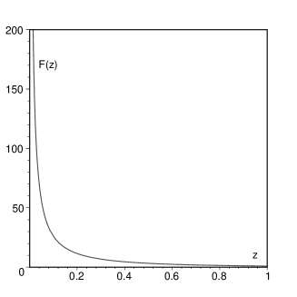
Figure 3: The spectral function $F(z)$.

One can also obtain the spectral distribution of radiation by integrating (100) over the variable $\beta$, which can be extended to the full axis in view of the exponential decay of the integrand. The result reads:

$$\frac{1}{l}\frac{dP^{0}}{d\omega}=\frac{16\pi^{5}f^{6}d}{3\gamma\mu^{2}}F(z),\quad z=\frac{\omega d}{\gamma\kappa},$$ (104)

where

$$F=(8z^{2}+8z+6)\frac{{\rm e}^{-z}}{\sqrt{\pi z}}+(8z^{2}+12z+6-3/z)({\rm erf}(\sqrt{z})-1).$$ (105)

The spectrum is shown on the Fig. 3. For small frequencies $\omega\ll\gamma\kappa/d$ the function $F(z)$ has a logarithmic divergence

$$F(z)\sim\frac{3}{z},$$ (106)

while for large $z$ it decays exponentially

$$F(z)\sim\frac{12{\rm e}^{-z}}{\sqrt{\pi z^{3}}}.$$ (107)

Finally, the total radiation per unit length is obtained by integrating (104) over frequencies using a cutoff length $\Delta$:

$$\frac{1}{l}P^{0}=\frac{16\pi^{5}f^{6}\kappa}{3\mu^{2}}\phi(y),\quad y=\frac{d}{\gamma\kappa\Delta},$$ (108)

where

$$\phi(y)=12\sqrt{\frac{y}{\pi}}\,{{}_{2}F_{2}}\left(\frac{1}{2},\frac{1}{2};\frac{3}{2},\frac{3}{2};-y\right)-3\ln\left(4y{\rm e}^{C}\right)+\frac{7}{2},$$ (109)

where the generalized hypergeometric function is used. The function $\phi(y)$ is plotted on Fig. 4, for small $y$ the leading term is the logarithm, while the asymptotic value for large $y$ is $\phi(\infty)=7/2$.

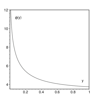
Figure 4: Dependence of radiation energy on the impact parameter, $y={d}/({\gamma\kappa\Delta})$.

The speed of the effective radiation source $v_{p}$ tends to infinity when the two strings become parallel. In this case (corresponding to $\kappa=\gamma$ in the above formula) the Cerenkov cone opens up to $\theta=\pi/2$, and the whole picture becomes essentially $2+1$ dimensional. Since this case is in fact generic (superluminal strings can be always “parallelized” by the world-sheet reparameterizations (III) and suitable space-time Lorentz transformations), this gives an alternative description of the effect as bremsstrahlung under collision of charges in $2+1$ electrodynamics.

VI Bremsstrahlung in 2+1 electrodynamics

Classical system of parallel strings interacting via the antisymmetric two-form potential $B_{\mu\nu}$ can be equivalently presented as the system of point charges interacting via the Maxwell field $A_{\mu}$ in 2+1 dimensions (in what follows in this section the Greek indices run over $\mu=0,1,2$). Indeed, substituting the constraint into the action (2) and assuming that all variables are $x^{3}$-independent, one can rewrite the action as

$$S=-\sum_{n=1,2}\int\limits\left(m_{n}d\tau_{n}+e_{n}A_{\mu}dx_{n}^{\mu}\right)-\frac{1}{4}\int\limits F_{\mu\nu}F^{\mu\nu}d^{3}x.$$ (110)

The correspondence between the quantities here and in the previous section looks as follows:

$$A_{\mu}=\sqrt{2l}B_{3\mu},\quad m_{n}=\mu_{n}l,\quad e_{n}=2\sqrt{2l}\pi f_{n},$$ (111)

and $F_{\mu\nu}=\partial_{\mu}A_{\nu}-\partial_{\nu}A_{\mu}$, where $l$ is the normalization length along the suppressed coordinate $x^{3}$. The equations of motion in the gauge $\partial_{\mu}A^{\mu}=0$ read

$$m_{n}\ddot{x}^{\mu}_{n} = e_{n}{F^{\mu}}_{\nu}\dot{x}^{\nu}_{n},$$ (112)

$$\square A^{\mu} = -J^{\mu},$$ (113)

where $J^{\mu}=J_{1}^{\mu}+J_{2}^{\mu}$,

$$J^{\mu}_{n}=e_{n}\int\limits\dot{x}_{n}^{\mu}\delta^{3}(x-x_{n}(\tau_{n}))d\tau_{n},$$ (114)

and only mutual interaction should be taken in the particle equations of motion after the classical mass renormalization.

Performing standard calculations we obtain for the energy loss under particle collision:

$$P^{\mu}=\frac{1}{8\pi^{2}}\int\limits k^{\mu}\frac{k^{0}}{|k^{0}|}\delta(k^{2})|J_{\mu}(k)|^{2}d^{3}k.$$ (115)

In $2+1$ dimensions a photon has the unique polarization state, so alternatively this expression can be rewritten (after integration over $k^{0}$) as

$$P^{\mu}=\frac{1}{8\pi^{2}}\int\limits\frac{k^{\mu}}{|{\bf k}|}|J({\bf k})|^{2}d^{2}k,$$ (116)

where we put $k^{0}=|{\bf k}|,\;e^{\mu}=(0,{\bf e}),\;J({\bf k})=J_{\mu}({\bf k})e^{\mu}$, and two-dimensional vectors are parameterized as

$${\bf k} = \omega\,[\cos\varphi,\sin\varphi],$$

$${\bf e} = [-\sin\varphi,\cos\varphi].$$ (117)

Perturbation theory with respect to the formal charge parameter $e$ (whose dimension in the $2+1$ electrodynamics is $l^{-1/2}$ in the units $\hbar=c=1$) is constructed in the same way as in the Sec. II, introducing the input world-lines

$$_{0}x^{\mu}_{n}=d^{\mu}_{n}+u^{\mu}_{n}\tau_{n},$$ (118)

with space-like impact vectors $d^{\mu}_{n}$ and unit time-like 3-velocities $u^{\mu}_{n}$:

$$u^{\mu}_{1}=[1,0,0],\quad u^{\mu}_{2}=\gamma[1,0,-v].$$ (119)

After the first iteration one obtains

$${}_{1}x^{\mu}_{1}=\frac{ie_{1}e_{2}}{4\pi^{2}m_{1}}\int\limits\frac{u_{2}^{\mu}(qu_{1})-q^{\mu}(u_{1}u_{2})}{q^{2}(qu_{1})^{2}}\delta(qu_{2}){\rm e}^{iq(d-u_{1}\tau_{1})}d^{3}q,$$ (120)

where $d=d_{2}-d_{1}$, and similarly for the second charge. The first order current, which gives the lowest order contribution to radiation, reads

$${}_{1}J^{\mu}=\sum_{n=1,2}e_{n}\int\limits d\tau_{n}\left({}_{1}{\dot{x}}^{\mu}_{n}-{u^{\mu}_{n}}\,_{1}x^{\nu}_{n}\partial_{\nu}\right)\delta\left(x-{{}_{0}x_{n}}(\tau_{n})\right).$$ (121)

Its Fourier-transform is

$$_{1}J^{\mu}(k)=\frac{e_{1}e_{2}}{2\pi}\int\delta(qu_{2})\delta[(k-q)u_{1}]{\rm e}^{i(d_{1}k+qd)}\left(\frac{e_{1}}{m_{1}}Q^{\mu}_{1}+\frac{e_{2}}{m_{2}}Q^{\mu}_{2}\right)d^{3}q,$$ (122)

where

$$Q^{\mu}_{1} = \frac{(ku_{1})^{2}u_{2}^{\mu}-(ku_{1})(ku_{2})u_{1}^{\mu}+(u_{1}u_{2})[(kq)u_{1}^{\mu}-(ku_{1})q^{\mu}]}{q^{2}(ku_{1})^{2}},$$

$$Q^{\mu}_{2} = \frac{(ku_{2})^{2}u_{1}^{\mu}-(ku_{1})(ku_{2})u_{2}^{\mu}+(u_{1}u_{2})[(kq)u_{2}^{\mu}-(ku_{2})(k-q)^{\mu}]}{(k-q)^{2}(ku_{2})^{2}}.$$ (123)

Integration over $q$ is performed similarly as in the case of strings: two delta-functions are used to integrate over $q^{0},\,q^{2}$, the remaining integral over $q^{1}$ is evaluated using a contour integration in the complex plane. Finally, projecting the amplitude on the polarization vector $e^{\mu}$ we obtain

$$_{1}J({\bf k})=\frac{e_{1}e_{2}}{2\omega\gamma v}\left(\frac{e_{1}{\rm e}^{-\omega d/v\gamma+ikd_{1}}}{m_{1}}(-\cos\varphi+i\gamma\sin\varphi)-\frac{e_{2}{\rm e}^{-\omega d\xi/v+ikd_{2}}}{m_{2}\gamma^{2}\xi^{2}}\left[\cos\varphi-i(v\xi\gamma^{2}+\sin\varphi)\right]\right),$$ (124)

where $\xi=1+v\sin\varphi$.

As we argued in the Sec. 3, our iteration scheme converges if the relative velocity is relativistic, and for cosmological applications one is interested by moderately relativistic velocities when $\gamma$ is not large. However, for general $\gamma$ it is difficult to perform computation of the total energy loss analytically, so we continue calculations in the ultrarelativistic case $\gamma\gg 1$ when additional simplifications can be made. Hopefully this should give a reasonable approximation for $\gamma$ of the order of several units. One can show that then the second term in (124) is dominant (the asymmetry of contributions from the first and the second charges is due to our choice of the reference frame: the first charge is at rest before the collision, while the second is moving with the relativistic velocity). The spectral distribution of radiation due to the second term extends till $\omega\sim 2\gamma^{2}/d$ in the narrow angular region $\delta\varphi\sim 1/\gamma$ around the direction $\varphi=-\pi/2$, while the first term has a lower ($\sim\gamma/d$) frequency cutoff. The total contribution of the second term to the radiation loss is greater than that of the first one by a factor of $\gamma$, so in what follows we neglect the first term. Setting $e_{1}=e_{2}=e,\,m_{1}=m_{2}=m$ we find from the Eq. (116) the spectral-angular distribution of radiation as follows

$$\frac{dP^{0}}{d\omega d\varphi}=\frac{1}{32\pi^{2}}\frac{e^{6}}{m^{2}}\frac{\left[\cos^{2}\varphi+(\sin\varphi+\xi\gamma^{2})^{2}\right]{\rm e}^{-2\omega d\xi}}{\omega\gamma^{6}\xi^{4}}.$$ (125)

For $\gamma\gg 1$, radiation is peaked in the direction of motion of the relativistic charge $\varphi=-\pi/2$, and in the vicinity of this direction (cf.(86))

$$\xi\thickapprox\frac{1}{2}(\gamma^{-2}+\beta^{2}),$$ (126)

where $\beta\ll 1$, and

$$\frac{dP^{0}}{d\omega d\beta}=\frac{e^{6}\gamma^{2}}{8\pi^{2}m^{2}\omega}\frac{(1-\gamma^{2}\beta^{2})^{2}}{(1+\gamma^{2}\beta^{2})^{4}}\exp\left({-\frac{\omega d(1+\gamma^{2}\beta^{2})}{\gamma^{2}}}\right).$$ (127)

The spectrum has an infrared divergence, and in the forward direction $\beta=0$ it extends up to $\omega\sim\omega_{{\rm max}}$, where

$$\omega_{{\rm max}}=\frac{\gamma^{2}}{d}.$$ (128)

Integrating over frequencies from the infrared cutoff $\Delta^{-1}$ we obtain

$$\frac{dP^{0}}{d\beta}=\frac{e^{6}\gamma^{2}}{8\pi^{2}m^{2}}\frac{(1-\gamma^{2}\beta^{2})^{2}}{(1+\gamma^{2}\beta^{2})^{4}}{\rm Ei}\left(1,\frac{d(1+\beta^{2}\gamma^{2})}{\gamma^{2}\Delta}\right).$$ (129)

Taking into account relations (111) between parameters of 3+1 and 2+1 problems, one can see that this expression coincides with (102) for $\gamma=\kappa$, i.e. for $\alpha=0$:

$$\frac{1}{l}\frac{dP^{0}}{d\beta}=\frac{64\pi^{4}f^{6}\gamma^{2}}{\mu^{2}}\frac{(1-\gamma^{2}\beta^{2})^{2}}{(1+\gamma^{2}\beta^{2})^{4}}{\rm Ei}\left(1,\frac{d(1+\beta^{2}\gamma^{2})}{\gamma^{2}\Delta}\right).$$ (130)

VII Cosmological estimates

In the standard axion cosmology scenario, which assumes the Peccei-Quinn phase transition after inflation, the global string network is formed at the temperature $T_{0}\sim f$. Strings initially move with substantial friction DS87 ; VI91 ; MaSh97 due to scattering of particles present in the hot cosmic plasma. At some temperature $T_{*}<{f}$ the string network enters the scale-invariant regime HS91 ; Na97 ; YKY98 when strings move almost freely with relativistic velocities AlTu ; Sh87 and are able to form closed loops via interconnections. Finally, at much lower temperature $T_{1}$ of the QCD phase transition, axions become massive and strings disappear. Our mechanism presumably should work in the temperature interval $(T_{*},\,T_{1})$, though an additional contribution from the damped epoch $T_{0}<T<T_{*}$ can also be expected. The scaling density of strings is determined from numerical experiments, it can be presented as

$$\rho_{s}=\frac{\zeta\mu}{t^{2}},$$ (131)

with $\zeta$ varying from 1 to 13 in different simulations.

Our aim is to estimate the total energy density $\varepsilon_{a}$ of axions produced via the bremsstrahlung mechanism during the cosmological period from $t_{*}$ (corresponding to temperature $T_{*}$) till the QCD phase transition moment $t_{1}$. These are commonly estimated as BaSh97

$$t_{*}({\rm sec}) \sim 10^{-20}\left(\frac{f}{10^{12}{\rm GeV}}\right)^{-4},$$ (132)

$$t_{1}({\rm sec}) \sim 2\cdot 10^{-7}\left(\frac{f}{10^{12}{\rm GeV}}\right)^{1/3}.$$ (133)

Consider the scattering of an ensemble of randomly oriented straight strings on a selected target string in the rest frame of the latter. Since the dependence of the string bremsstrahlung on the inclination angle $\alpha$ is smooth, we can use for a rough estimate the particular result obtained for the parallel strings ($\alpha=0$) introducing an effective fraction $\nu$ of “almost” parallel strings (roughly 1/3). Then, if there are $N$ strings in the normalization cube $V=L^{3}$, we have to integrate the radiation energy released in the collision with the impact parameter $d=x$ over the plane perpendicular to the target string using the measure $N/L^{2}\cdot 2\pi xdx$. Actually we need the radiation power per unit time, so, for an estimate, we have to divide the integrand on the impact parameter. This quantity should be multiplied by the total number of strings $N$ to get the radiation energy released per unit time within the normalization volume. Therefore, for the axion energy density generated per unit time we obtain:

$$\frac{d\varepsilon_{a}}{dt}=\int_{0}^{L}P^{0}\,\nu\,\frac{N}{L^{2}}\,\frac{N}{V}\,2\pi dx.$$ (134)

As an expression for $P^{0}$ we will use here the Eq. (108), and we have to integrate over the impact parameter. Taking into account that the string number density is related to the energy density (131) via

$$\frac{N}{V}=\frac{\rho_{s}}{\mu L},$$ (135)

introducing the integral

$$\xi(w) = \int_{0}^{w}\phi(y)dy=12\sqrt{\frac{w}{\pi}}\Biggl{[}\ _{2}F_{2}\left(-\frac{1}{2},-\frac{1}{2};\frac{1}{2},\frac{3}{2};-w\right)-$$ (136)

$$- {{}_{2}F_{2}}\left(-\frac{1}{2},-\frac{1}{2};\frac{1}{2},\frac{1}{2};-w\right)\Biggr{]}+\left(\frac{13}{2}-3\ln\left(4w{\rm e}^{C}\right)\right)w,$$

and using for $\mu$ the expression (11) with only the second (leading) term, we obtain

$$\frac{d\varepsilon_{a}}{dt}\sim Kf^{2}\gamma^{3}\xi(w)\frac{1}{t^{3}\ln^{2}(tf)},$$ (137)

where

$$K=\frac{8}{3}\pi^{4}\nu\zeta^{2},\quad w=\frac{L}{\gamma^{2}\Delta}.$$ (138)

Since in the cosmological context $L\sim\Delta\sim t$, one can take $w=\gamma^{-2}$ for an estimate.

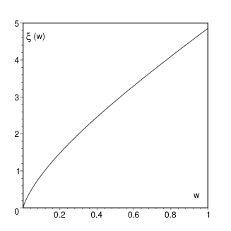
Figure 5: Dependence of the axion radiation rate on the Lorentz factor of the collision $\xi(w),\,w=L/(\gamma^{2}\Delta)$.

The realistic value of $\gamma$ is of the order of unity, while our formulas were obtained in the $\gamma\gg 1$ approximation, since we were keeping only the second term in the exact amplitude (V). But an independent calculation shows that for $\gamma\sim 1$ the contribution from the first term is of the same order, so we can hope to get reasonable order of magnitude estimate using the above formulas for $\gamma$ not large. The full $\gamma$-dependence is given by the function $\gamma^{3}\xi(\gamma^{-2})$, where $\xi(w)$ is plotted on Fig. 5. For $\gamma=\sqrt{2}$

$$\gamma^{3}\xi(\gamma^{-2})\approx 8.137,$$ (139)

while for $\gamma=5$

$$\gamma^{3}\xi(\gamma^{-2})\approx 55.83.$$ (140)

Another source of uncertainty is the numerical value of the parameter $\zeta$, which was obtained in different simulations within the region between 1 and 13. Now we have to integrate the radiation power over time from $t_{*}$ to $t_{1}$ as given by (132) and (133). Using the integral (with substitution $x=1/t$)

$$\int\limits\frac{x}{\ln^{2}x}dx=-\frac{x^{2}}{\ln x}+2{\rm Li}(x^{2}),$$ (141)

where the logarithmic integral function is introduced, which for large $x$ is equal approximately to

$$-\frac{x^{2}}{\ln x}+2{\rm Li}(x^{2})\approx\frac{x^{2}}{2\ln^{2}x},$$ (142)

we find the energy density of axions at the moment $t_{1}\gg t_{*}$:

$$\varepsilon_{a}\sim\frac{Kf^{2}\gamma^{3}\xi(w)}{2t_{*}^{2}\ln^{2}(t_{*}/t_{0})},$$ (143)

where the ratio $t_{*}/t_{0}$ can be estimated as

$$\frac{t_{*}}{t_{0}}=\left(\frac{m_{\rm Pl}}{f}\right)^{2}.$$ (144)

Finally, dividing by the critical energy density at $t=t_{1}$

$$\varepsilon_{\rm cr}=\frac{3m_{\rm Pl}^{2}}{32\pi t_{1}},\quad m_{\rm Pl}=1.22\cdot 10^{19}{\rm GeV},$$ (145)

we obtain the following estimate for the relative contribution of bremsstrahlung axions

$$\Omega^{\rm br}_{a}\sim 0.5\cdot 10^{16}\left(\frac{\zeta}{13}\right)^{2}\left(\frac{f}{10^{12}{\rm GeV}}\right)^{32/3},$$ (146)

where we have used the value (139). This estimate shows that our new mechanism is very sensitive to the value of $f$ and gives an upper bound on axion window of the order of $10^{10}{\rm GeV}$. We postpone more precise cosmological estimates for a separate publication. In particular, more careful analysis is needed to find radiation loss for moderately relativistic string velocities.

VIII Conclusions

In this paper, we have suggested a new mechanism for the axion emission by the global string network: the bremsstrahlung under string collisions. As far as we are aware, this effect was not discussed in the context of the cosmic string scenario so far. Though it is of the second order in the axion coupling constant, rough cosmological estimates show that it is not small and gives a contribution of the same order of magnitude as radiation due to oscillating loops.

We have found the radiation amplitude using the perturbation theory whose validity is restricted by relativistic (though not necessarily ultrarelativistic) velocities of colliding strings. The frequency spectrum has an infrared divergence which is not an artifact of our approximation, but rather is the effect of the space-time dimensionality: as we have shown, an equivalent description of the axion bremsstrahlung from strings in $3+1$ dimensions is provided by the electrodynamics of point charges in $2+1$ dimensions, where its origin lies in the logarithmic dependence on distance of the Coulomb potential. Unfortunately the integration over the spectrum and the angular distribution can be performed analytically only in the ultrarelativistic case, and the final formulas obtained relate to this situation. But, in view of a smooth dependence of the radiation efficiency on the Lorentz factor of the collision, we hope that our results give a reasonable estimate of the effect for values of the Lorentz factor of the order of several units as well.

From a purely theoretical viewpoint two aspects are worth to be discussed. The first is the Cerenkov nature of radiation which is associated with the possibility of the superluminal motion of an effective source located around the point of minimal separation between the strings. In perturbative setting, the strings, which are straight in zero order approximation, get deformed under axion interaction, with the deformation being maximal near this point. This region therefore acts as an effective source of radiation arising in the next order approximation. This explains why radiation is concentrated on the Cerenkov cone directed along the trajectory of the effective source. Another interesting feature is that the effect has an alternative $2+1$ interpretation as the bremsstrahlung of point charges. This is due to the fact that two strings inclined with respect to each other and moving in the superluminal regime can be made parallel by suitable reparameterizations of their world-sheets and the choice of the space-time Lorentz frame. This transformation is only feasible once the relative string motion is superluminal in the sense described above. Classical dynamics of parallel strings interacting via the axion field in $3+1$ dimensions is equivalent to dynamics of point charges in $2+1$ electrodynamics, therefore the string axion bremsstrahlung is reduced to the point particle bremsstrahlung in lower dimension.

References

- (1) R. Peccei and H. Quinn, CP conservation in the presence of pseudoparticles, Phys. Rev. Lett. 38, 1440 (1977), and Constraints imposed by CP conservation in the presence of pseudoparticles, Phys. Rev. D16, 1791 (1977).
- (2) S. Weinberg, A new light boson, Phys. Rev. Lett. 40, 223 (1978).
- (3) F. Wilczek, Problem of strong P and T invariance in the presence of instantons, Phys. Rev. Lett. 40, 279 (1978).
- (4) L. Abbot and P. Sikivie, A cosmological bound on invisible axion, Phys. Lett. B120, 133 (1983); J. Preskill, M. Wise, and F. Wilczek, Cosmology of the invisible axion, Phys. Let. B120 127 (1983); M. Dine and W. Fischler, The not so harmless axion, Phys. Lett. B120 137 (1983).
- (5) M. Srednicki, Axions: past, present and future, in Proceedings of the International Conference on Continuous advances in QCD, Minneapolis 2002, edited by K. A. Olive, M. A. Shifman, M. B. Voloshin (Singapore, World Scientific, 2002.), p. 509; hep-th/0210172.
- (6) P. Sikivie, Axions and their distribution in galactic halos, Invited talk at 4th International Workshop on the Identification of Dark Matter (IDM 2002), York, England, 2002, 10pp.; hep-ph/0211254.
- (7) J. E. Kim, Light pseudoscalars, particle physics and cosmology, Phys. Rep. 150, 1 (1987); H.-Y. Cheng, The strong CP problem revisited, Phys. Rep. 158, 1-158 (1988); M. S. Turner, Windows on the axion, Phys. Rep. 197, 67-97 (1990); G. G. Rafflet, Astrophisical methods to constrain axions and other novel particle phenomena, Phys. Rep. 198, 1 (1990).
- (8) A. E. Everett, Cosmic strings in unified gauge theories, Phys. Rev. D24, 858 (1981).
- (9) A. Vilenkin, Cosmic strings and domain walls, Phys. Rep. 121, 263 (1985).
- (10) G. V. Gibbons, S. W. Hawking and T. Vachaspati eds., The formation and evolution of cosmic strings, (CUP, 1990).
- (11) A. Vilenkin and E. P. S. Shellard, Cosmic strings and other topological defects, (CUP, 1994).
- (12) M. B. Hindmarsh and T. W. B. Kibble, Cosmic strings, Rept. Prog. Phys. 58, 477-562 (1995); hep-ph/9411342.
- (13) R. A. Battye and E. P. S. Shellard, Recent perspectives on axion cosmology, in Proceedings of the International Conference on Dark Matter in Astro- and Particle Physics, Heidelberg, 1996, edited by H. V. Kladpor-Kleingrothaus (World Scientific, 1997), p. 554; astro-ph/9706014.
- (14) E. P. S. Shellard and R. A. Battye, Cosmic axion, in Proceedings of COSMO 97: 1st International Workshop on Particle Physics and the Early Universe, Ambleside, England, 1997, edited by L. Roszkowski (Singapore, World Scientific, 1998), p. 233; astro-ph/9802216.
- (15) J. E. Kim, Cosmic axion, Talk given at 2nd International Workshop on Gravitation and Astrophysics, Tokyo, Japan, 1997; astro-ph/9802061.
- (16) R. A. Battye and E. P. S. Shellard, Axion string cosmology and its controversies, in Proceedings of the 2nd International Conference Physics Beyond The Standard Model: Beyond The Desert 99: Accelerator, Non-accelerator And Space Approaches into the Next Millenium, Ringberg Castle, Tegernsee, Germany, 1999, edited by H. V. Klapdor-Kleingrothaus and I. V. Kirvosheina (Bristol, UK, Inst. Phys., 2000), p. 565; Astro-ph/9909231.
- (17) R. L. Davis and P. Sikivie, On the evolution of global strings in the early universe, Phys. Lett. B195, 361 (1987).
- (18) A. Vilenkin, Cosmic string dynamics with friction, Phys. Rev. D43, 1060 (1991).
- (19) C. J. A. P. Martins and E. P. S. Shellard, String evolution with friction, Phys. Rev. D53 575 (1996); hep-ph/9507335.
- (20) C. Hagmann and P. Sikivie, Computer simulations of the motion and decay of global strings, Nucl. Phys. B363, 247 (1991).
- (21) M. Nagasava, Scaling distribution of axionic strings and estimation of axion density from axionic domain walls, Prog. Theor. Phys. D8, 851 (1997); hep-ph/9712341.
- (22) M. Yamaguchi, M. Kawasaki, and J. Yokoyama, Evolution of axionic strings and spectrum of axions radiated, Phys. Rev. Lett. 82, 4578 (1998); hep-ph/9811311; M. Yamaguchi, Scaling property of the global string in the radiation dominated univers, Phys. Rev. D60, 103511 (1999); hep-ph/9907056.
- (23) A. Albrecht and N. Turok, Evolution of cosmic strings, Phys. Rev. Lett. 54, 1868 (1885).
- (24) E. P. S. Shellard, Cosmic string interactions, Nucl. Phys. 283, 624 (1887).
- (25) R. L. Davis, Goldstone bosons in string models of galaxy formation, Phys. Rev. D32, 3172 (1985); Cosmic axions from cosmic strings, Phys. Lett. B180, 225 (1985).
- (26) D. Garfinkle and T. Vachaspati, Radiation of goldstone bosons from cosmic strings, Phys. Rev. D36, 2229 (1987); E. Copeland, D. Haws, and E. Hindmarsh, Classical theory of radiating strings, Phys. Rev. D42, 726 (1990).
- (27) R. L. Davis and E. P. S. Shellard, Do axions need inflation?, Nucl. Phys. B324, 167 (1989).
- (28) M. Sakellariadou, Gravitational waves emitted from infinite strings, Phys. Rev. D42, 354 (1990); Radiation of Nambu-Goldstone bosons from infinitely long cosmic strings, Phys. Rev. D44, 3767 (1991).
- (29) A. Dabholkar and M. Quashnock Pinning down the axion, Nucl. Phys. B333, 815 (1990).
- (30) R. A. Battye and E. P. S. Shellard, Axion string constraints, Phys. Rev. Lett. 73 , 2954 (1994): (E) ibid., 76, 2203 (1996); Global string radiation, Nucl. Phys. B423, 260 (1994).
- (31) M. Yamaguchi, M. Kawasaki, and J. Yokoyama, Evolution of axionic strings and spectrum axion radiated from them, Phys. Rev. Lett. 82, 4578 (1999).
- (32) C. Hagmann, S. Chang, and P. Sikivie, Axion from string decay, Nucl. Phys. B, Proc. Suppl. 72, 81 (1999)
- (33) C. Hagmann, S. Chang, and P. Sikivie, Axion radiation from strings, Phys. Rev. D63, 125018 (2001); hep-ph/0012361.
- (34) D. V. Gal’tsov, Yu. V. Grats, and P. S. Letelier, Post-linear formalism for gravitating strings: crossed straight strings collision, Ann. of Phys. 224, 90 (1993).
- (35) D. V. Gal’tsov, Yu. V. Grats, and A. B. Lavrent’ev, Cerenkov radiation of superconducting cosmic strings, Pis’ma Zh. Eksp. Teor. Fiz. 59, 359 (1994); JETP Lett. 59, 385 (1994).
- (36) R. Kerner, J. W. van Holten, and R. Colistete Jr, Relativistic Epicycles : another approach to geodesic deviations, Class. Quant. Grav. 18, 4725 (2001); gr-qc/0102099.
- (37) R. A. Battye and E. P. S. Shellard, String radiative backreaction, Phys. Rev. Lett. 75, 4354 (1995).