Cosmic Shear from STIS pure parallels

Following the detection of a cosmic shear signal at the 30^′′ scale using archival parallel data from the STIS CCD camera onboard HST in Hämmerle et al. (2002), we analyzed a larger data set obtained from an HST GO pure parallel program. Although this data set is considerably larger than the one analyzed previously, we do not obtain a significant detection of the cosmic shear signal. The potential causes of this null result are the multiple systematics that plague the STIS CCD data, and in particular the degradation of the CCD charge transfer efficiency after 4 years in space.

1 Introduction

This is the third of a series of articles describing the use of parallel observations with the STIS CCD camera onboard the HST for the detection of cosmic shear on scales below one arcmin. The first 2 papers (Pirzkal et al. 2001, hereafter PCE01, and Hämmerle et al. 2002, hereafter HMS02) were centered on the analysis of data carefully selected from the HST archive, spanning a period between 1997 and 1998. These first 2 papers established that the STIS CCD camera used in the CLEAR mode is a useful instrument to measure the value of the cosmic shear at scales (30^′′) where ground-based observations are not efficient. The significance of value obtained in HMS02 for the rms shear, $\sqrt{\left\langle\overline{\gamma}^{2}\right\rangle}=3.87^{+1.29}_{-2.04}\%$, was limited by the number of galaxies in usable fields. To strengthen the constraint and decrease the error bars in the shear estimate, we needed more usable fields. This led us to propose for further observations in parallel mode. This paper concentrates on the analysis of data obtained from a Cycle 9 dedicated pure parallel GO proposal. Throughout this paper, we employ the same formalism developed in HMS02, and we refer the reader to that paper for the complete mathematical description of the terms used. The paper is organized as follows: In Sect. 2, we describe the characteristics of the data obtained. Sect. 3 addresses the field selection and catalog production. Sect. 4 is dedicated to the number counts and sizes of galaxies. In Sect. 5 we analyse the PSF anisotropy. Sect. 6 describes the shear analysis, including the PSF corrections applied. In Sect. 7 we discuss the results obtained, and we concentrate on the understanding of the different effects which influence it. Finally, in Sect. 8, we summarize our results and try to offer a perspective on the future works using STIS and ACS.

2 Data

Figure 1: Half-light radius in STIS subsampled pixels vs. S/N for 2 star fields. On the left panel the association had a dither pattern between members, while on the right the offsets between members were less than 1 pixel. The strip at $r_{\mathrm{h}}<1$ on the right panel indicates the presence of individual hot pixels. The strip at 2.1$<$ $r_{\mathrm{h}}<$ 2.6 is populated by stars.

The data which was used for the analysis in this paper was obtained as part of parallel GO proposal (8562+9248 P.I.: P. Schneider) from Sept. 24th 2000 until May 16th 2001. The latter date corresponds to the moment when a fuse in the primary power feed of STIS blew up, stopping instrument operations until July 2001 when STIS was repowered through the secondary power line.

A total of 3511 individual datasets were obtained during this period. Each individual image was bias substracted and flat-fielded automatically on request by the data archive at the Space Telescope Science Institute using the On-the-Fly Calibration process (Crabtree et al. (1996)) with the best available calibration data. The images were then associated following the definition given in PCE01 into 575 STIS associations (Micol et al. (1998)). Each association includes data which were taken consecutively during a single telescope visit using the same telescope roll angle, and which were offset by no more than one quarter of the field-of-view. The relative offsets between members of the associations were computed using the available jitter data and refined using the same iterative cross-correlation technique as described in PCE01. Each image in the association was drizzled using the IRAF STSDAS DRIZZLE procedure in a subsampled grid with a scale of 0.5 input pixels and offset to register the different members. The final associated image was obtained by the median average of the members of the association using the IRAF IMCOMBINE procedure. During this step, we used CRREJECT to reject pixels with a deviation larger than 3$\sigma$ from the mean value. This last step was necessary for this dataset since it was no longer taken in CR-SPLIT mode as it was the case for the data used in PCE01 and HMS02.

Of these 575 associations, 568 have a total exposure time larger than 400s. The mean exposure time for an association is about 2500s. This has to be compared to the mean exposure time of the archival data associations which was about 2000s. Another intrinsic difference between the archival data analyzed and the newly obtained data is that it was no longer obtained in the CR-SPLIT mode and therefore we need at least 2 consecutive single exposures of the same field to be able to properly remove cosmic rays. We limited our analysis then to the 484 associations for which we have at least 2 members. All those datasets can be found on http://www.stecf.org/projects/shear/

Still we can see from Fig. 1 that some images, for which the members are not dithered by more than 1 pixel, are contaminated by a number of hot pixels. Between 1997-1998, when the archival data was taken, and the period 2000-2001, when the cycle 9 data was obtained, the number of hot pixels was increased by a factor of 4 (see Fig. 1 in Proffitt et al. 2002a). This increase in number has made it very difficult for the hot pixels to be cleaned up from non-dithered images. Those hot pixels which are isolated can be identified as they form a strip with half-light radius of less than one subsampled STIS pixel. Therefore they can be rejected when we select objects (stars and galaxies) by their half-light radius. However, a number of hot pixels will lay inside objects, affecting their shape measurement. Because the distribution of those pixels is random, when averaging, they will affect the noise in our measurement, increasing the dispersion of ellipticities.

Besides this higher contamination from hot pixels, the degradation in the charge transfer efficiency (CTE) between 1997 and 2000 has to be considered also. The radiation to which the CCD is subjected in space degrades the capability of the charges to be successfully moved through adjacent pixels. This effect is characterized by a loss of flux in objects with increasing distance to the read-out amplifier, which for our data is located at the top-right. This loss of efficiency is particularly strong in the Y direction as shown by Goudfrooij et al. (2002) and negligible in the X direction. This leads to the apparition of visible trails parallel to the Y direction for bright stars as can be seen in Fig. 2. The effect of the degradation of the CTE is discussed in more detail in Sect. 7.3.

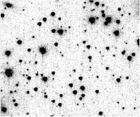
Figure 2: Snapshot of one of the starfields where the CTE degration can be clearly seen in the form of trails originating from the stars and parallel to the Y direction.

3 Field selection and catalogue production

The co-added associations were inspected visually and classified as either star fields or galaxy fields in the same fashion as done in PCE01. The final selection included 210 galaxy fields and 110 star fields. The complete list of star and galaxy fields can be found on http://www.stecf.org/projects/shear/

The fields were analyzed in the same way as in HMS02 which is summarized in the following: SExtractor (Bertin & Arnouts 1996) catalogues were produced using the parameter file which can be found at http://www.stecf.org/projects/shear/sextractor. We discarded all objects flagged internally by SExtractor due to problematic deblending and/or thresholding, and we removed all objects located at less than 25 subsampled STIS pixels from the edges of the images which are highly noisy. Furthermore, we applied manual masks to problematic regions like diffraction spikes from saturated stars. IMCAT (Kaiser et al. 1995, Hoekstra et al. 1998, Erben et al. 2001) catalogues were produced parallely and merged with the cleaned SExtractor catalogues, requiring an object to be uniquely detected in both catalogues within a radius of 125 mas (5 subsampled STIS pixels) from the coordinates as defined by the SExtractor catalog. In the final merged catalog, we use the size (half-light radius $r_{\mathrm{h}}$) and shape parameters (Luppino & Kaiser 1997; Hoekstra et al. 1998) from IMCAT, with the position and the magnitude defined by SExtractor.

We identified stars with the same parameters as in the data presented in HMS02: 2.1$<$ $r_{\mathrm{h}}<$2.6 and S/N$>$10. For the galaxies, we applied a slightly more conservative criterion of $r_{\mathrm{h}}>$2.7 and S/N$>$5.

4 Galaxy number counts and sizes

Figure 3: Number of detected galaxies per STIS association as a function of total exposure time in seconds for the 210 galaxy fields.

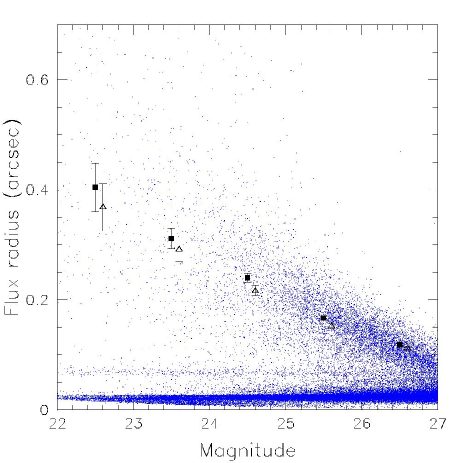
Figure 4: Half-light radius as measured by SExtractor for the objects detected in the galaxy fields as a function of the CLEAR filter AB magnitude. The horizontal strip at a half-light radius between 0$.\!\!^{\prime\prime}$05 and 0$.\!\!^{\prime\prime}$08 is caused by stars and other unresolved objects. The strip at the half-light radius between 0$.\!\!^{\prime\prime}$025 and 0$.\!\!^{\prime\prime}$03 is a product of the single noise pixels, mostly hot-pixels. The average size of galaxies (objects with a half-light radius greater than 0$.\!\!^{\prime\prime}$08) per magnitude bin are indicated by the full squares. The error bars represent the 3$\sigma$ level in the error of the mean. The open triangles represent the same for the fields studied in PCE01 and HMS02.

In Fig. 3, we plot the number of detected galaxies per associated image as a function of total exposure time. When compared with the archival data, the average total exposure time is higher, 2500s, leading to a higher mean number of galaxies per field of 24 (35 gal/arcmin²). The average exposure time is very close to the optimal integration time deduced from the archival data up to which the number of galaxies detected per field rises steadily as a function of integration time. After that, the number of galaxies detected rises more slowly because the intrisic flattening of galaxy number counts at faint magnitudes and because of those faint objects become too small to be resolved by STIS.

This effect can be seen also in Fig. 4, where the half-light radius measured by SExtractor of the objects in galaxy fields as a function of the magnitude is plotted. The average half-light radius for galaxies varies from 0$.\!\!^{\prime\prime}$37 for magnitude bin 22-23 to 0$.\!\!^{\prime\prime}$1 for magnitude bin 26-27. Those values are consistent with what was found in PCE01 and in Gardner & Satyapal (2000). Beyond magnitude 27, most of the objects become unresolved for STIS and therefore cannot be used for our analysis.

5 Analysis of the PSF anisotropy

Since the expected distortion of image ellipticities on the STIS angular scale should be a few percent, any instrumental distortion and other causes of PSF anisotropy need to be controled to an accuracy of better than 1%. We showed in HMS02 that the STIS PSF anisotropy remained remarkably stable and was sufficiently small (less than 1%) in amplitude between June 1997 and October 1998. We analyzed the PSF properties of the newly obtained data to check whether this remained the case. We show in Fig. 5 the mean ellipticities of stars, $e_{1}$ and $e_{2}$ as defined in Eq. (3) of HMS02, over the whole field as a function of the epoch. The variation of the PSF anisotropy in time is similar to what was found in HMS02 for the period 1997-1998. For the stars, the mean $e_{1}$ is about 1% and the mean $e_{2}$ is close to 0, with a dispersion of about 1%. Therefore, we consider the PSF anisotropy to be constant over the period of time covered.

We investigated also the spatial variation of the PSF within invidual fields. We show a characteristic star field in Fig. 6. We applied the same procedure described in HMS02 [Eqs. (5) and (6)] of fitting a second-order polynomial to the ellipticity of a star at each star position on the CCD. Comparing this with Fig. 4 and 5 of HMS02, we find that the anisotropy patterns and their dispersions are similar for both datasets.

Figure 5: Mean ellipticity components $e_{1}$, on the left, and $e_{2}$, on the right, of the star fields vs. epoch of the observations in Modified Julian Date. The straight solid line shows for the mean over all the fields, with the dashed lines showing the 1$\sigma$ dispersion. The circles show the mean for star fields in 3 different time bins together with the 1$\sigma$ error bars for those values. The black triangles indicate the fields that were selected for the PSF correction.

Figure 6: For the star field o6fx9j010_2.ass, we show the distribution of the ellipticities of stars before (top left) and after (top right) correcting for the PSF anisotropy using the fitted second order polynomial plotted on the bottom right panel. The bottom left panel shows the original spatial distribution of the ellipticities. The length of the sticks indicates the modulus of the ellipticity and the orientation gives the position angle.

6 Shear analysis

6.1 PSF anisotropy correction

From the 110 star fields obtained, we selected 14 for the PSF correction of galaxies. This selection was done with the same criteria as for the archival data: good spatial coverage of stars and small intrinsic dispersion in star ellipticities. This allows us to have a good fit to the anisotropy pattern and to minimize the noise in the PSF correction. The galaxy ellipticities were corrected for anisotropy; the formalism can be found in Eqs. (14), (15), (16) and (17) of HMS02. Each galaxy in each galaxy field is corrected by one of the selected star fields. Averaging over all the galaxies, we obtain a mean anisotropy corrected ellipticity for each galaxy field with a particular star field correction. Then, averaging over the 14 different star fields corrections, we obtain an average value for the mean anisotropy corrected ellipticity for each galaxy field.

In Fig. 7, the mean ellipticity for the galaxies in all the galaxy fields is shown with and without the PSF anisotropy correction. The difference between the mean anisotropy corrected and uncorrected ellipticities is less than 1%. One trend emerges though, as the anisotropy correction shifts the mean ellipticities into the negative $e_{1}$ direction. This is not unexpected since there is a positive $e_{1}$ component on the star fields as seen in Fig. 5, which was also present in the archival data.

One big difference arises between this dataset and the archival data. The mean ellipticity, corrected or uncorrected, over all the galaxy fields is no longer compatible with 0 as it should be if the shear due to the large-scale structure is uncorrelated on the different galaxy fields, and the galaxies are oriented randomly intrinsically. We find $\left\langle e_{1}\right\rangle=(-1.03\pm 0.40)\%$ and $\left\langle e_{2}\right\rangle=(-0.32\pm 0.38)\%$ for the uncorrected ellipticities and $\left\langle e^{\mathrm{ani}}_{1}\right\rangle=(-1.29\pm 0.40)\%$ and $\left\langle e^{\mathrm{ani}}_{2}\right\rangle=(-0.40\pm 0.38)\%$ for the anisotropy corrected ellipticites, where the errors given are calculated as errors on the mean as $\sigma/\sqrt{N}$, not taking into account the dispersion from the different PSF corrections. The deviation from zero for the $e_{1}$ component is 3$\sigma$ significant and indicates the presence of a systematic effect in the galaxy fields.

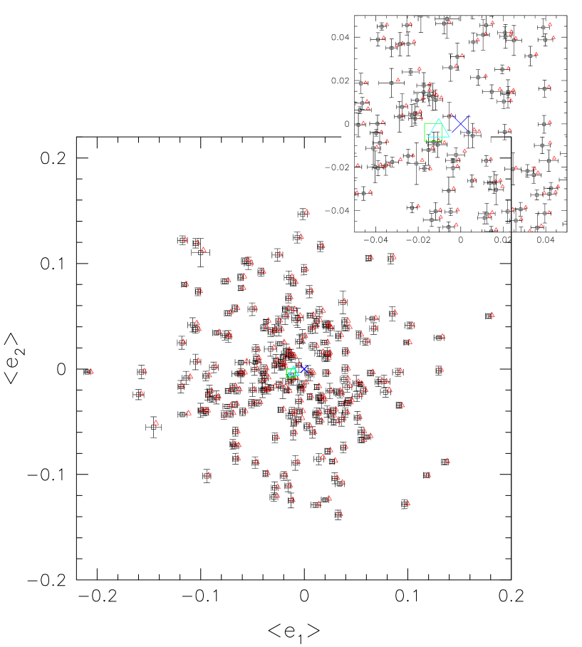
Figure 7: For the 210 galaxy fields, we plot the mean uncorrected ellipticity of galaxies (triangles) as well as the mean anisotropy corrected ellipticity (squares). The error bars on the squares indicate 3 times the dispersion of the field-averaged corrected ellipticities with the different PSF model fits. The error on the mean is in reality smaller than the symbols used. The big triangle and the big square at the center show the mean over all galaxy fields of respectively the uncorrected and corrected mean ellipticities. Their size represent the 1$\sigma$ errors on the mean. The cross marks the 0,0 point. For clarity, a zoom on the central part is showed on the upper right corner.

6.2 Smearing correction and fully corrected ellipticities

The fully corrected ellipticity is obtained from the anisotropy corrected ellipticities by $\mathrm{e}^{\mathrm{iso}}=(P^{\gamma})^{-1}e^{\mathrm{ani}}$ [Eq. (18) in HMS02], where $P^{\gamma}=P_{\mathrm{sh}}-(P_{\mathrm{sh}}/P_{\mathrm{sm}})^{\star}P_{\mathrm{sm}}$ [Eq. (15) in HMS02]. We apply a scalar inversion of this tensor $(P^{\gamma})^{-1}=2/{\rm{tr}}P^{\gamma}$ which is less noisy than the full tensor inversion as demonstrated in Erben et al. (2001). Therefore to compute the fully corrected ellipticity of each galaxy, we need to calculate $P^{\gamma}$ for each galaxy, and for this purpose we need to estimate the ratio of the shear and smear susceptibility tensors $(P_{\mathrm{sh}}/P_{\mathrm{sm}})^{\star}$ from the light profile of the stars with the filter scale of the galaxy [see Eq. (1) in HMS02]. We find no spatial variation of $(P_{\mathrm{sh}}/P_{\mathrm{sm}})^{\star}$ for any filter scale over the selected star fields as it was the case for the archival data. But there are variations between the different star fields, closely related to the average size of the stars, r${}_{\mathrm{h}}=2.35\pm 0.25$ subsampled STIS pixels, which are compatible from field to field within the error bar. Taking the mean over all the 14 selected star fields for different filter scales, we show in Fig. 8 the dependence of $(P_{\mathrm{sh}}/P_{\mathrm{sm}})^{\star}$ on the filter scale. This ratio increases with the filter scale and becomes constant for large objects. This is intuitively expected since small objects are going to be more affected by the PSF smearing and therefore are going to have a larger $P^{*}_{\mathrm{sm}}$. The dependence shown for the Cycle 9 data is similar to the one for the archival data and the values are compatible within the error bars.

Figure 8: The mean of $(P_{\mathrm{sh}}/P_{\mathrm{sm}})^{\star}$ over all 14 stars fields which were used for the PSF correction is shown for different filter scales. The error bars show the dispersion between different star fields.

Since to fully correct the ellipticities, one has to divide by $P^{\gamma}$, objects with small values of $P^{\gamma}$ can get unphysically large ellipticities. Those can dominate the cosmic shear signal even after the introduction of a weighting scheme which is discussed in the following section. Therefore, we decided, as in HMS02, to introduce a cut in $P^{\gamma}$, requiring that “good” galaxies should have $P^{\gamma}>0.2$ and $\left|e\right|<1$. The effects of this cut are discussed in Sect. 7.1. As for the archival data, each galaxy field is corrected with each of the selected starfields. The dispersion of the corrected galaxy ellipticities using the different starfield corrections is only about 1%. The mean PSF fully corrected ellipticity is then obtained by averaging over all the individual corrections. When averaging over all the galaxies, we find that $\left\langle e^{\mathrm{iso}}_{1}\right\rangle=(-1.41\pm 0.41)\%$ and $\left\langle e^{\mathrm{iso}}_{2}\right\rangle=(-0.34\pm 0.41)\%$ where the error quoted is the error on the mean given by the statistical dispersion of the ellipticities divided by the square root of the total number of galaxies. The dispersion of ellipticities is found to be 26$\%$ for both components as it was the case for the archival data.

6.3 Weighting scheme

The PSF corrections, anisotropy and smearing, applied to the galaxy ellipticities amplify the measurement error of these values. This can lead for certain objects to unphysical ellipticities. The goal of the weighting is to minimize the impact of those high-ellipticity objects which are most likely to originate from noise. The adopted procedure is the same as we used for the data on HMS02. Since we expect galaxies with small sizes and/or low S/N to be the most sensitive to noise, we search for each galaxy the 20 nearest neighbours in the (r_h, S/N) parameter space (Erben et al. 2001) and calculate the dispersion of their fully-corrected ellipticities which we call $\sigma_{\mathrm{NN}}$. The weight is then just defined as $w_{\mathrm{NN}}=1/{\sigma_{\mathrm{NN}}}^{2}$. Even in the case of a perfect measurement and a perfect PSF correction, there would be a dispersion in the shear estimate, $\sigma_{\mathrm{g}}$, because of the contribution of the intrinsic ellipticity dispersion of the galaxy population $\sigma_{\mathrm{s}}$. Therefore, since $\sigma_{\mathrm{NN}}$ is an estimate of $\sigma_{\mathrm{g}}$ , it can be never lower than $\sigma_{\mathrm{s}}$. This leads to an upper limit for the weights given by:

$$w_{\mathrm{NN}}^{\prime}=\mathrm{min}\left(\frac{1}{\sigma_{\mathrm{NN}}^{2}},\frac{1}{\sigma_{\mathrm{s}}^{2}}\right)$$ (1)

with $\sigma_{\mathrm{s}}$ = $\sqrt{2}\times 26\%$ as measured from the distribution of the corrected galaxy ellipticities.

6.4 Cosmic Shear estimation

The fully corrected ellipticity is an unbiased (but noisy) estimate of the shear. We use it to calculate an estimator of the shear variance for each of the $n$ galaxy fields by calcultating a weighted average of the galaxy ellipticities $\overline{\gamma}^{2}_{n}:=\frac{\sum_{i\neq j}w_{in}w_{jn}\mathrm{e}_{in}\mathrm{e}_{jn}^{*}}{\sum_{i\neq j}w_{in}w_{jn}}$ [Eq. (9) of HMS02]. By calculating the weighted average over all the galaxy fields, we obtain the estimated cosmic shear for our data $\left\langle\overline{\gamma}^{2}\right\rangle=\frac{\sum{N_{n}\overline{\gamma}^{2}}}{\sum{N_{n}}}$ [Eq (11) in HMS02], where $N_{n}$ is the number of galaxies per field. The associated statistical error $\sigma_{\left\langle\overline{\gamma}^{2}\right\rangle}$ is defined in Eq. (21) of HMS02. The results are summarized in Table 1 for all selected galaxy fields and for fields with more than 10 or more than 15 galaxies per field, with different cuts in $P^{\gamma}$ and with different weightings.

The cosmic shear estimator for the analyzed data is negative or close to 0 in almost all the cases for different selections and weighting schemes of the galaxies and the galaxy fields. For the 121 fields in HMS02, we found $\left\langle\overline{\gamma}^{2}\right\rangle=(14.96\pm 11.61)\times 10^{-4}$ using all fields and all galaxies with $P^{\gamma}>0.2$, while we find for the 210 galaxy fields of cycle 9 data and using the same selection and correction criteria $\left\langle\overline{\gamma}^{2}\right\rangle=(-7.16\pm 5.13)\times 10^{-4}$. This value is certainly surprising since it is negative for a value that is positively defined. But one has to remember that we compute only an estimator of the real shear variance which even if it is unbiased can be found negative if it is dominated by noise and systematics.

The variance of the cosmic shear in a circular aperture $\theta/2$ can also be calculated from the correlation function $\left\langle\gamma\gamma\right\rangle$ for the scale $\theta$ (Bartelmann & Schneider, 2001) in an indepedent way from the estimator $\left\langle\overline{\gamma}^{2}\right\rangle$. As shown in Fig. 9, where we plot the integrated values for the correlation function, $\left\langle\gamma\gamma\right\rangle$ is consistenly negative confirming the result found from the cosmic shear estimator. It has to be noted though that since we plot the integrated correlation function, points are not independent from each other.

Another way to estimate the significance of the estimator is to randomize the orientation of the galaxies in all the galaxy fields and weight them in the same way than for the measured result. The probability distribution function for the cosmic shear estimator obtained in that way is shown on Fig. 10. In 93.4$\%$ of the randomizations, the value is higher than the measured one, confirming then that the negative value for the cosmic shear estimator is not significant statistically. The full width at half maximum of the distribution is about $5\times 10^{-4}$ which agrees with the errors estimated from the intrinsic ellipticity distribution, $\sigma_{\mathrm{intr}}=\frac{\sigma_{\mathrm{s}}^{2}}{N\sqrt{N_{\mathrm{f}}}}=4\times 10^{-4}$, where $N$ is the average number of galaxies per field plus the error from the cosmic variance $\sigma^{2}_{\mathrm{cv}}=\frac{\left\langle\overline{\gamma}^{2}\right\rangle}{\sqrt{N_{\mathrm{f}}}}=5\times 10^{-5}$ .

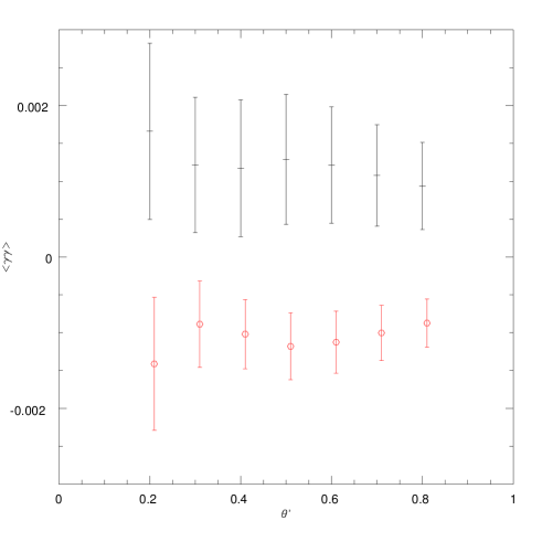
Figure 9: Integrated correlation function $\left\langle\gamma\gamma\right\rangle$ as a function of the scale in arcminutes for the Cycle 9 data (data points with a circle) and for the archival data of HMS02.

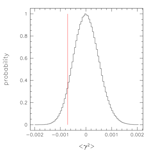
Figure 10: Probability distribution of the cosmic shear estimator calculated from the Cycle 9 data by randomizing the orientations of galaxies used for the cosmic shear analysis in all galaxy fields. Individual galaxies are weighted with $w^{\prime}_{\mathrm{NN}}$ and the galaxy fields are weighted by the number of galaxies on each field. The shape of the distribution looks very similar to the one calculated for the archival data, however, it is much narrower than for the archival data which is due to the higher total number of galaxies used in the measurement (note the different scalings of the plots). The vertical line indicates the measured cosmic shear value.

Table 1: Results for the cosmic shear estimates and errors for different minimum number of galaxies per field. $N$ is the number of galaxies per field, $N_{\mathrm{f}}$ is the number of galaxy fields with $N\geq N_{\mathrm{min}}$. The first block shows the results for different cuts in $P^{\gamma}$, where we weight individual galaxies with $w=w^{\prime}_{\mathrm{NN}}$ and the galaxy fields with $W_{\mathrm{f}}=N$. In the next blocks the results are given for weighting individual galaxies or not, and for applying different weights to galaxy fields, weighting them equally ($W_{\mathrm{f}}=1$), weighting by the number of galaxies per field ($W_{\mathrm{f}}=N$) or by the square of the number of galaxies ($W_{\mathrm{f}}=N^{2}$). The last two blocks show the results for different minimum sizes of the selected galaxies and when using only fields which were dithered by more than $1$ pixel. Note that we repeat the result with $r_{\mathrm{h}}>2.7$, $P^{\gamma}>0.2$, $w=w^{\prime}_{\mathrm{NN}}$, $W_{\mathrm{f}}=N$ in each block (except the last) for easier comparison of the results.

	all			$N\geq 10$			$N\geq 15$
	$N_{\mathrm{f}}$	$\left\langle\overline{\gamma}^{2}\right\rangle$	$\sigma_{\left\langle\overline{\gamma}^{2}\right\rangle}$	$N_{\mathrm{f}}$	$\left\langle\overline{\gamma}^{2}\right\rangle$	$\sigma_{\left\langle\overline{\gamma}^{2}\right\rangle}$	$N_{\mathrm{f}}$	$\left\langle\overline{\gamma}^{2}\right\rangle$	$\sigma_{\left\langle\overline{\gamma}^{2}\right\rangle}$
		$\times 10^{4}$	$\times 10^{4}$		$\times 10^{4}$	$\times 10^{4}$		$\times 10^{4}$	$\times 10^{4}$
different cuts in $P^{\gamma}$; $w=w^{\prime}_{\mathrm{NN}}$; $W_{\mathrm{f}}=N$; $r_{\mathrm{h}}>2.7$
$P^{\gamma}>0.0$	$210$	$-7.92$	$5.04$	$190$	$-6.48$	$5.04$	$142$	$-1.33$	$5.05$
$P^{\gamma}>0.1$	$210$	$-7.19$	$5.03$	$190$	$-5.46$	$5.06$	$137$	$0.61$	$5.17$
$P^{\gamma}>0.2$	$210$	$-7.16$	$5.13$	$184$	$-6.04$	$4.97$	$130$	$1.44$	$5.36$
different weighting of individual galaxies; $P^{\gamma}>0.2$; $W_{\mathrm{f}}=N$; $r_{\mathrm{h}}>2.7$
$w=1$	$210$	$-4.95$	$5.51$	$184$	$-3.21$	$5.40$	$130$	$4.11$	$5.76$
$w=w_{\mathrm{NN}}$	$210$	$-8.72$	$4.96$	$184$	$-8.14$	$4.74$	$130$	$-0.59$	$5.08$
$w=w^{\prime}_{\mathrm{NN}}$	$210$	$-7.16$	$5.13$	$184$	$-6.04$	$4.97$	$130$	$1.44$	$5.36$
different weighting of galaxy fields; $P^{\gamma}>0.2$; $w=w^{\prime}_{\mathrm{NN}}$; $r_{\mathrm{h}}>2.7$
$W_{\mathrm{f}}=1$	$210$	$-13.77$	$5.31$	$184$	$-10.41$	$4.95$	$130$	$1.82$	$5.43$
$W_{\mathrm{f}}=N$	$210$	$-7.16$	$5.13$	$184$	$-6.04$	$4.97$	$130$	$1.44$	$5.36$
$W_{\mathrm{f}}=N^{2}$	$210$	$-3.12$	$6.08$	$184$	$-2.79$	$5.98$	$130$	$1.06$	$6.18$
different cuts in half-light radius; $P^{\gamma}>0.2$; $W_{\mathrm{f}}=N$; $w=w^{\prime}_{\mathrm{NN}}$
$r_{\mathrm{h}}>2.7$	$210$	$-7.16$	$5.13$	$184$	$-6.04$	$4.97$	$130$	$1.44$	$5.36$
$r_{\mathrm{h}}>3$	$210$	$-7.31$	$6.01$	$181$	$-7.56$	$5.26$	$120$	$1.90$	$5.21$
$r_{\mathrm{h}}>4$	$210$	$-8.41$	$8.02$	$148$	$-3.98$	$7.79$	$78$	$3.66$	$8.78$
$r_{\mathrm{h}}>5$	$210$	$-5.20$	$14.41$	$83$	$12.19$	$11.91$	$34$	$15.24$	$19.51$
using only fields dithered by $>1$ pixel; $P^{\gamma}>0.2$; $W_{\mathrm{f}}=N$; $w=w^{\prime}_{\mathrm{NN}}$; $r_{\mathrm{h}}>2.7$
	$95$	$-2.39$	$7.93$	$87$	$-1.47$	$7.33$	$61$	$1.85$	$7.79$

7 Discussion

The negative cosmic shear estimate that we find when considering all the fields, if not a statistical fluke, can only be due to selection effects or systematics present in our data. We review in the following the possible causes of systematics and try to assess their impact.

7.1 Selection and weighting effects

To verify the validity of the data reduction, which is somewhat different from the one used on the first 2 papers, we simulated 210 associations with an average of 24 galaxies per field using Skymaker (Erben et al. 2001) in a similar fashion as described in Sect. 5.4 of HMS02. Each associations consists of 4 members with relative random shifts between 0 and 3 pixels which are coadded in the same way as the real data. We found that, as for the archival data in HMS02, the final cosmic shear estimate is 2.4% with a 3$\sigma$ significance as compared to the 2.6% true shear introduced in the simulated galaxy catalogs. We estimate then that the reduction procedure is completely equivalent for our purposes and is not responsible for the negative shear estimate.

We investigated if this negative value could be the product of the way that fields are selected. Since parallel imaging pointings are controlled by the observations of the primary instrument, one could think that we may be biased towards a certain category of fields. We did 100.000 random selections of 121 fields (the number of fields in HMS02) out of the 210 available and computed the mean of the cosmic shear estimator for these fields. The distribution of the obtained values is shown in Fig. 11. A value as large as the one obtained in the analysis of the archival data from HMS02 could be obtained in just 0.003% of the realisations.

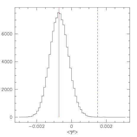
Figure 11: Distribution of the cosmic shear estimator calculted from 121 randomly selected fields out of the 210. The vertical solid line represents the value of the estimator for this data, while the vertical dashed line represents the value of the estimator for the data measured in HMS02

In Table 1, we summarize the results for different selections of fields, different cuts in $P^{\gamma}$, different weightings of individual galaxies and galaxy fields. If we calculate the estimator by varying the cuts in $P^{\gamma}$, no significant variation is obtained, which indicates that the measurement is not dominated by a few noisy galaxies with large correction factors. The effect of the weighting of individual galaxies is more significant since the estimator becomes more negative when a weighting is applied (with no difference between $w^{\prime}_{\mathrm{NN}}$ and $w_{\mathrm{NN}}$. If we vary the weighting of the galaxy fields, the dispersion is minimized for a Poisson noise weighting $W_{\mathrm{f}}=N$, though the estimator is less negative with $W_{\mathrm{f}}=N^{2}$. We observe, as it was the case in HMS02, that the shear estimate increases when we select fields with a larger number density of galaxies, which are typically deeper exposures for which we expect galaxies to be on average at a larger redshift and therefore the true shear signal to be higher. This effect was also seen in the archival data. It indicates then that even if our estimator is negative, a true shear signal may be present in our data.

7.2 Hot pixels

The impact of hot pixels can be seen in in the last 2 blocks of Table 1. When using objects with a larger r_h, which are less affected by left-over hot pixels, or fields where exposures are dithered by more than 1 pixel (which can be cleaned of hot pixels), the cosmic shear estimate increases slightly. But since the number of galaxies is also reduced, the dispersion of the result is higher and therefore not significant. We have to note also that for larger objects, the observed behaviour could be due also to CTE effects as discussed later.

7.3 PSF effects

The effect of each individual star field PSF correction on the final shear estimate result is presented on Table 2. As seen in the first block of Table 2, even in the absence of PSF corrections, the cosmic shear estimate has a negative value, and the full correction of the PSF just decreases even more the value of the estimate. We observe that the final result does not vary significantly between the different corrections and that all results are well within the statistical error of the shear estimate. The effect of the PSF correction for most of the fields is rather small as can be seen in Fig. 12. As a test, we applied the PSF correction as estimated from the archival star fields to the Cycle 9 galaxy fields. And vice-versa, we applied PSF correction as estimated from the Cycle 9 star fields to the galaxy fields from HMS02. In both case we found no significant variation of the result in the cosmic shear estimate.

Figure 12: We show for each of the 210 galaxy fields the cosmic shear estimator as a function of the number of galaxies. The vertical error bars indicate the 1$\sigma$ dispersion from the mean. The horizontal error bars indicate the variation in the number of objects depending on the cut in $P^{\gamma}$

Table 2: Results for the cosmic shear estimator for different PSF corrections, weighting individual galaxies with $w=w^{\prime}_{\mathrm{NN}}$, requiring $P^{\gamma}>0.2$ (or $P_{\mathrm{sh}}>0.2$), and weighting the galaxy fields by $W_{\mathrm{f}}=N$. Note that even after the cut in $P^{\gamma}$ some galaxies are left with unphysical ellipticities larger than one which were excluded from the analysis. This leads to the different number of galaxy fields for $N\geq 10$ and $N\geq 15$ in the first block, where we show the results if we do not correct for PSF effects: the first column indicates if we use uncorrected (raw) ellipticities ($\mathrm{e}^{\mathrm{raw}}$) or anisotropy-corrected ellipticities ($\mathrm{e}^{\mathrm{ani}}$) and if we apply the smearing correction ($P^{\gamma}$) or not ($P_{\mathrm{sh}}$). The first row gives the fully corrected result (see Table 1) for reference. The next block shows the results when we apply PSF corrections from the individual star fields.

$e$, $P$	all			$N\geq 10$			$N\geq 15$
or	$N_{\mathrm{f}}$	$\left\langle\overline{\gamma}^{2}\right\rangle$	$\sigma_{\left\langle\overline{\gamma}^{2}\right\rangle}$	$N_{\mathrm{f}}$	$\left\langle\overline{\gamma}^{2}\right\rangle$	$\sigma_{\left\langle\overline{\gamma}^{2}\right\rangle}$	$N_{\mathrm{f}}$	$\left\langle\overline{\gamma}^{2}\right\rangle$	$\sigma_{\left\langle\overline{\gamma}^{2}\right\rangle}$
starfield		$\times 10^{4}$	$\times 10^{4}$		$\times 10^{4}$	$\times 10^{4}$		$\times 10^{4}$	$\times 10^{4}$
$\mathrm{e}^{\mathrm{ani}}$, $P^{\gamma}$	$210$	$-7.16$	$5.13$	$184$	$-6.04$	$4.97$	$130$	$1.44$	$5.36$
$\mathrm{e}^{\mathrm{raw}}$, $P^{\gamma}$	$210$	$-8.12$	$5.07$	$184$	$-7.08$	$4.91$	$131$	$-0.42$	$5.30$
$\mathrm{e}^{\mathrm{ani}}$, $P_{\mathrm{sh}}$	$210$	$-1.25$	$2.07$	$203$	$-0.99$	$2.08$	$181$	$-0.06$	$2.14$
$\mathrm{e}^{\mathrm{raw}}$, $P_{\mathrm{sh}}$	$210$	$-1.80$	$1.99$	$206$	$-1.68$	$2.00$	$186$	$-0.94$	$2.05$
o6969zaz0_3_ass	$210$	$-7.59$	$5.55$	$182$	$-6.22$	$5.31$	$127$	$1.28$	$5.83$
o696nnmu0_2_ass	$210$	$-5.24$	$4.97$	$186$	$-4.33$	$4.84$	$133$	$2.10$	$5.26$
o696surs0_3_ass	$210$	$-7.39$	$5.40$	$182$	$-6.02$	$5.19$	$128$	$2.28$	$5.68$
o6fx9j010_2_ass	$210$	$-5.90$	$5.13$	$186$	$-4.94$	$4.97$	$132$	$2.06$	$5.44$
o6fxc7f30_4_ass	$210$	$-8.10$	$5.52$	$182$	$-6.81$	$5.32$	$129$	$0.73$	$5.91$
o6fxdeng0_1_ass	$210$	$-8.95$	$5.65$	$182$	$-7.72$	$5.40$	$125$	$-0.90$	$5.88$
o6fxdmeo0_2_ass	$210$	$-7.62$	$5.43$	$183$	$-6.04$	$5.22$	$129$	$1.25$	$5.71$
o6fxdsrr0_2_ass	$210$	$-8.49$	$5.48$	$182$	$-7.13$	$5.29$	$128$	$0.88$	$5.84$
o6fxe5xq0_3_ass	$210$	$-6.14$	$5.07$	$186$	$-5.11$	$4.92$	$133$	$1.16$	$5.37$
o6fxebok0_3_ass	$210$	$-6.18$	$5.11$	$186$	$-5.15$	$4.98$	$133$	$1.24$	$5.47$
o6fxep010_2_ass	$210$	$-6.84$	$5.05$	$186$	$-5.81$	$4.91$	$133$	$0.46$	$5.37$
o6fxfohi0_2_ass	$210$	$-5.43$	$4.81$	$186$	$-4.72$	$4.69$	$133$	$1.58$	$5.10$
o6fxfuh50_2_ass	$210$	$-5.98$	$5.00$	$186$	$-5.05$	$4.86$	$132$	$1.62$	$5.30$
o6fxheu90_2_ass	$210$	$-5.64$	$5.02$	$186$	$-4.73$	$4.90$	$133$	$1.65$	$5.33$

7.4 CTE effects

As stated in Sect. 2, the CTE of the STIS CCD has been degradating by about 15% per year on average since 1997 (Goudfrooij et al. 2002, Proffitt et al. 2002b). This degradation is characterized by a loss in the efficiency of the transfer of charges in the Y direction, which is related to the distance of the pixel from the read-out amplifier, the number of charges of the pixel and the number of charges between the pixel and the read-out amplifier. This effect is responsible for a loss of flux for all objects, but in particular for faint objects in a low background environment (Goudfroij et al. 2002). We expect then that, for our galaxies which are a few counts over the sky background, this may affect also their shapes by introducing a correlation between $e_{1}$ and the Y position of the galaxies. If we plot, like in Fig. 13, the average $e_{1}$ for all the galaxies as a function of Y, we observe that the closer the galaxies are to the bottom of the chip, the more they tend to be aligned towards the Y direction. This correlation was not seen in the archival data (PCE01). The fact that big galaxies, with $r_{\mathrm{h}}>5$, seem to be less affected than small galaxies by the systematics causing the estimator to be negative as shown in Table 1 is also consistent with the way CTE degradation acts.

To estimate the effect of CTE degradation on the cosmic shear estimate for our data, we simulated ten thousand times 200 fields with 25 galaxies per field, with the observed ellipticity dispersion and with a mean $e_{1}=-0.01$. We added a y-depence to $e_{1}$ in order to simulate an average CTE degradation with the form: $e_{1}=-0.15+0.3\times y/2000$. This is about 5 times the CTE degradation seen for the average of all the galaxies. For one set of simulations we had no cosmic shear effect and for a second set we added a shear of 2.5%, and we computed the distribution of $\left\langle\overline{\gamma}^{2}\right\rangle$ for each set. As can be seen in Fig. 14, the effect of CTE degradation is to lower $\left\langle\overline{\gamma}^{2}\right\rangle$. However, this is a worst case scenario where we assumed that the mean corrected $e_{1}$ is smaller than the maximum CTE induced ellipticities. Also, this average CTE degradation alone cannot produce a negative signal as large as the one observed even in the case where the shear is 0. But since this effect depends not only on the position but also on the flux of each galaxy, the background as well as on the date when the images where taken, only a physical model of the CTE degradation which would take into account all those parameters could allow us to estimate its true impact (P. Bristow, private communication). We tried to correct the CTE degradation effect in the same way as in van Waerbeke et al. (2000), by adding a constant term to $e_{1}$ as a function of the Y-position (and/or background, surface brightness) of the galaxy in order to have the mean value of $e_{1}$ over all galaxies to be 0. This method does not work in this case and the value of cosmic shear estimator remains negative. To do a proper correction, it would be necessary to restore each single image using a physical model of the CTE degradation which is not available yet.

Figure 13: Average $e_{1}$ for all galaxies as a function of the X-position (bottom box) and Y-position (top box) in the field for bins of 200 subsampled STIS pixels. The error bars represent the variation on the mean.

Figure 14: Cosmic shear estimator distribution for the simulated catalogs with a 2.5% true shear (thick lines) and without (thin lines) shear. Full lines indicate the distribution for the catalogs including the average CTE effect and the dashed lines the distribution for the catalogs without CTE effect. The arrow indicates the position of the measured cosmic shear estimate from the real data.

8 Summary and Perspectives

Following the analysis of the 210 galaxy fields selected from the Cycle 9 parallel proposal, we have found that the cosmic shear estimate $\left\langle\overline{\gamma}^{2}\right\rangle$ is consistently negative and therefore the cosmic shear signal is not detected on the scale of 30^′′. Only fields with more than 15 galaxies per field yeld a positive $\left\langle\overline{\gamma}^{2}\right\rangle$ though it is not statistically significant. This is most likely due to the existance of several systematics that plague the STIS, however we cannot exclude that this negative result is largely due to a statistical fluke. We have studied several sources of noise and systematics that could contaminate this result: selection and weighting effects, hot pixels, PSF effects and degradation of the CTE. Neither of those seem to have by themselves the power to turn the estimate negative at the level observed in the presence of a significant signal (more than 1%). But it appears also that the main effect for this negative result comes from the loss of charge transfer efficiency of the STIS CCD. Several groups (Goudfrooij & Kimble 2002, Bristow et al. 2002) are trying to come up with physical models to correct for this effect and restore the images. Once these models will be publicly available, it will be interesting to try to model in detail the real effect of the charge transfer inefficiency on the shapes of individual galaxies. If it turns out that the difference observed between the results of data analysed in HMS02 and this one comes principally from the loss of CTE, then it would be important for future studies with space-based telescopes (SNAP, JWST) to prioritize these observations during the first periods of use of the instruments in order to minimize its impact.

Is it useful now to try to correct these STIS images for the cosmic shear measurements? Since the installation of the ACS camera onboard HST in March 2002, parallel data is also being acquired with it. The area covered by those observations already surpasses all the area covered with the analysed Cycle 9 pure parallel STIS data. We expect then the ACS data will better constrain the cosmic shear at the same scale than STIS since it will finally cover a much larger area at a similar or even greater depth without being contaminated, for the time being, by the effect of CTE loss. Also, since the ACS field of view is about 3.5^′, it will be possible to cross-check its results with the available ground-based surveys at scales larger than the arcmin.

- (1) Bartelmann, M. & Schneider, P., 2001, Phys.Rep., 340, 291
- (2) Bertin, E. & Arnouts, S., 1996, A&AS, 117, 393
- Bristow et al. (2002) Bristow, P., Alexov, A., Kerber, F., Rosa, M., 2002, Proceedings of the 2002 HST Calibration Workshop, S. Arribas, A. Koekemoer, & B. Whitmore, eds., 177
- Crabtree et al. (1996) Crabtree, D.R., Durand, D., Gaudet, S., and Hill, N., 1996, ADASS V, A.S.P. Conf. Ser., George H. Jacoby and Jeannette Barnes, eds., 101, 505.
- (5) Erben, T., van Waerbeke, L., Bertin, E., Mellier, Y. & Schneider, P., 2001, A&A, 366, 717
- (6) Fruchter, A.S. & Hook, R.N., 2002, PASP, 114, 144
- (7) Gardner, J.P. & Satyapal, S., 2000, AJ 119, 2589
- (8) Goudfrooij, P. & Kimble, R.A., 2002, Proceedings of the 2002 HST Calibration Workshop, S. Arribas, A. Koekemoer, & B. Whitmore, eds., 105
- (9) Hämmerle, H., Miralles, J.-M., Schneider, P. et al., 2002, A&A, 385, 743 (HMS02)
- (10) Hoekstra, H., Franx, M., Kuijken, K. & Squires, G., 1998, ApJ, 504, 636
- (11) Hudson, M.J., Gwyn, S.D.J., Dahle, H. & Kaiser, N., 1998, ApJ, 503, 531
- (12) Kaiser, N., 1992, ApJ, 388, 272
- (13) Kaiser, N., 1998, ApJ, 498, 26
- KSB (95) Kaiser, N., Squires, G. & Broadhurst, T., 1995, ApJ, 449, 460
- (15) Luppino, G.A. & Kaiser, N., 1997, ApJ, 475, 20
- Micol et al. (1998) Micol, A., Pirenne, B., & Bristow, P., 1998, ADASS VII, A.S.P. Conf., R. Albrecht, R.N. Hook & H.A. Bushouse, eds., 145, 45
- (17) Pirzkal, N., Collodel, L., Erben, T., et al., 2001, A&A, 375, 351 (PCE01)
- (18) Proffitt, C. R., Goudfrooij, P., Brown, T. M., et al., 2002a, Proceedings of the 2002 HST Calibration Workshop, S. Arribas, A. Koekemoer, & B. Whitmore, eds., 97
- (19) Proffitt, C., et al. 2002, ”STIS Instrument Handbook”, Version 6.0, Baltimore: STScI
- (20) Rhodes, J., Refregier, A. & Groth, E.J., 2001, ApJL, 552, 85
- (21) van Waerbeke, L., Mellier, Y., Erben, T., et al., 2000, A&A, 358, 30