Complex X-ray spectral behaviour of NGC 4051 in the low flux state

Abstract

The Narrow Line Seyfert 1 galaxy NGC 4051 was observed in one of its prolonged low-lux states by XMM-Newton in November 2002. Here we present the results of an analysis of EPIC-pn data obtained during the observation. Within the low state, the source shows complex spectral variability which cannot easily be explained by any simple model. However, by making a ‘flux-flux’ plot which combines the low state data with data obtained during a normal flux state, we demonstrate that the extremely hard spectrum observed above 2 keV results from a continuation of the spectral variability seen in the normal state, which is caused by spectral pivoting of the power-law continuum. The pivoting power-law appears to be attached to a Comptonised thermal component of variable flux (blackbody temperature $kT\sim 0.1$ keV, consistent with the small black hole mass in NGC 4051) which dominates the soft X-ray band in the low state, and is probably the source of seed photons for Comptonisation. Additional constant thermal and reflection components, together with absorption by ionised gas, seem to be required to complete the picture and explain the complex X-ray spectral variability seen in the low state of NGC 4051.

1 Introduction

NGC 4051 is a low luminosity (typically few $10^{41}$ erg s^-1) Narrow Line Seyfert 1 (NLS 1) AGN which shows extreme X-ray flux variability and associated strong spectral variability (e.g. 1996,2003), on both long and short time-scales. In particular, the source shows unusual low flux states, lasting weeks to months, during which the X-ray spectrum becomes extremely hard (photon index $\Gamma\sim 1$) above a few keV but is dominated by a much softer component ($\Gamma\sim 3$) at lower energies (1998, 1999). Previously, we reported results of a Chandra CCD observation of NGC 4051 in the low flux state (2003, henceforth U03) which revealed that, even in the low state, the hard and soft components were significantly variable and correlated with one another, and so could not originate primarily in extended emission, such as reflection from a torus and extended scattering medium. The Chandra image also clearly ruled out any significant extended emission on $\sim 100$ pc scales (confirming an earlier result based on a Chandra grating observation obtained in a normal flux state, 2001). In U03 we further noted that the unusual curvature at harder energies in the Chandra spectrum, when compared with a spectrum of the low state obtained by the Rossi X-ray Timing Explorer (RXTE), was consistent with the presence of a very prominent gravitationally redshifted diskline, suggesting that the reflection features from close to a black hole may remain constant in flux in NGC 4051 despite large changes in the continuum flux, as appears also to be the case in MCG–6-30-15 (2003,2003).

In U03 we suggested that the unusual spectral shape of the low state was simply a continuation to low fluxes of the normal spectral variability, i.e. with the spectrum hardening towards lower fluxes. In other words, the low flux state is probably not a physically distinct state, in the sense used to describe the states of e.g. X-ray binaries, and the extreme long-term X-ray spectral variability of NGC 4051 is likely produced by the same physical process as the short-term spectral variability. Using a model-independent method, the ‘flux-flux’ plot, (2003) find that the spectral variability of NGC 4051 in the 2-15 keV band is best explained by pivoting of the power-law continuum about an energy of $\sim 100$ keV, in addition to a hard constant component. This result contrasts with the X-ray spectral variability of other Seyferts, which is best explained by a constant hard component together with a variable component which does not pivot but maintains a constant shape (2003, 2003).

Observations of NGC 4051 in the low state allow us to test the limits of the spectral pivoting model suggested by (2003). In this paper, we present the results of an XMM-Newton Target of Opportunity Observation (TOO) of NGC 4051 obtained towards the end of a recent low state. We first demonstrate the complex spectral variability in the low state and then combine the low state data with data obtained during a normal state, to make a ‘flux-flux’ plot (, 2003) to test the pivoting model and determine whether the low state spectrum is consistent with spectral pivoting down to the lowest observed fluxes. We also investigate the presence of reflection features in the hard spectrum obtained during the low state, and then combine these results with the inferences we make from the flux-flux plots, to construct a simple broadband spectral model which can explain the observed spectral shape and variability of NGC 4051. Using spectral fits, we demonstrate how our model can explain the complex spectral variability observed within the low state. We will present spectral fits of our model over the entire observed flux range of NGC 4051 (i.e. including the normal state) in a future paper (Taylor et al., in prep.).

Figure 1: Recent 2-10 keV light curve of NGC 4051, obtained with RXTE monitoring (see 2003, 2003 for details). The time of the XMM-Newton TOO observation (and the 2-10 keV flux observed by XMM-Newton) is marked by a star.

2 Observation

Our continuing RXTE monitoring observations showed that NGC 4051 entered a low state, characterised by low flux and a small variability amplitude, for about a month in 2002 October-November (Fig. 1). On detecting that the source was in a low state with RXTE, we triggered a TOO observation with XMM-Newton, which observed the source on 2002 Nov 22, towards the very end of this low state. Although the 2-10 keV X-ray flux at the time is higher than observed earlier in the state, at $6\times 10^{-12}$ erg cm^-2 s^-1 it is comparable to that observed by Chandra during the 2001 Feb low state (U03). XMM-Newton observed NGC 4051 for $\sim 50$ ks with all instruments, but due to background flaring only the central 33 ksec of data was useful. We therefore extracted EPIC-pn data (both single and double pixel events) in this useful time range from a 42 arcsec radius circle centred on the X-ray source, as well as a source-free box outside the source region on the same chip for background subtraction. The EPIC instruments were operated using the Medium filter and the EPIC-pn was operated in Large Window Mode throughout the observation, and due to the faint nature of the source pileup effects are negligible. We do not use EPIC-MOS data in this analysis, in order that we may directly compare the EPIC-pn data obtained during the low state with that obtained during a normal state at an earlier epoch before the recent change in EPIC-MOS response. The EPIC-pn and EPIC-MOS cross-calibration shows systematic discrepancies (up to 10%) between the instruments below 1 keV, so that it is unclear which gives the best representation of the spectral shape at these low energies. We note however that as a consistency check we have also carried on the EPIC-MOS data the same spectral fits carried out on EPIC-pn data in Section 5, and the results of these fits do not change the basic conclusions we present here (i.e. the same model is found to apply although specific model parameters change slightly). A detailed analysis of the RGS spectrum of NGC 4051, obtained during the XMM-Newton observation of the low state is presented in a separate paper (Page et al., in prep.).

3 Lightcurves and broadband spectra

In Fig. 2 we show the background-subtracted EPIC-pn light curves of NGC 4051 in two energy bands (0.1-0.5 keV, which we shall call soft and 2-10 keV, which we shall call hard). We also show the varying softness ratio (soft/hard) of the two bands. The source shows clear flux variability and interesting spectral variability during the low state. In particular, during the large ‘flare’ early in the observation, the softness ratio does not change substantially, and similar behavior can be seen during a second weaker flare at $\sim 22$ ks. However, towards the end of the observation (after $\sim 26$ ks), when the source is fainter in both bands the source softens, as the hard flux decreases substantially while the soft flux barely changes. The source also hardens slightly in reponse to small hard ‘flares’ in the period between the two larger flares.

Figure 2: Soft and hard 500 s resolution light curves of NGC 4051, together with the softness ratio between the two bands. Dotted lines denote the low, medium and both high flux epochs used to examine spectral variability in more detail.

In order to investigate the spectral variability in more detail, we plot in Fig. 3 the unfolded (relative to a simple power-law) EPIC-pn spectra corresponding to the epochs delineated in Fig. 2, which correspond to three of the four distinct periods discussed above, and which we refer to as high1, medium, and low flux spectra. For clarity, we do not plot the high2 spectrum, which is somewhat intermediate in shape between the high1 and medium flux epoch spectra. The spectra have been unfolded through the instrument response with respect to a simple power-law ($\Gamma=2$) absorbed by Galactic neutral absorption ($N_{\rm H}=1.3\times 10^{21}$ cm^-2, 1989). As noted in U03, although unfolded X-ray spectra are always model-dependent, in the case of relatively high resolution CCD instruments such as the EPIC-pn, only sharp features such as edges are significantly misrepresented, while the general continuum shape is fairly well represented by the unfolded spectra. It can be seen immediately that the high flux epoch corresponds to an increase in the soft flux, below $\sim 0.7$ keV, with little difference in the soft spectral shape between low, medium and high flux epochs at those low energies. Above $\sim 2$ keV, the spectral shape varies significantly. Interestingly, in all epochs there is little change in the continuum around $\sim 1$ keV.

Clearly the spectral variability cannot be explained by any simple spectral model. For example, the constancy in flux around 1 keV might suggest some kind of pivot point around that energy, however the soft spectral shape at lower energies appears to be constant and is inconsistent with any low energy pivot. Also, the high and medium flux epoch spectra appear to converge above 5 keV, despite both spectra showing quite different soft normalisations. In order to clarify the nature of the spectral variability, and place it into context with the spectral variability seen at higher fluxes, we now apply the flux-flux plot method to the data.

Figure 3: Unfolded broadband spectra (see Section 3 for details) obtained during high1 (black line), medium (thick light grey line) and low (dark grey line) flux epochs within the low state. The spectra are plotted in units of energy$\times$flux-density, so that a flat slope corresponds to a photon index $\Gamma=1$. For clarity the spectra have been plotted as histograms and error bars omitted. The spectra have been unfolded with respect to a simple power-law absorbed by Galactic absorption (see text for details).

4 Flux-flux plots

Figure 4: Left panel: Unbinned HS flux-flux relation. Low state data is plotted with filled markers, normal state data with lighter, open markers. For clarity only the 0-20 count/s soft flux range is plotted, although all data (extending to 45 count/s) is included to produced the binned relation (right panel). Right panel: Binned HS flux-flux relation. The dotted line shows the best-fitting power-law plus constants model described in the text.

(2003) used a simple, model-independent technique, the ‘flux-flux’ plot, to examine the nature of the X-ray spectral variability of Seyfert galaxies. Specifically, by plotting the flux in a hard band versus flux in a soft band, a linear relationship reveals that the data are consistent with a simple two-component model, where one component varies in flux but not in spectral shape, while the other component remains constant in spectral shape and flux (see also 2003, 2002). The spectral variability is then produced by a change in the relative normalisations of the two components, with hardening at low fluxes corresponding to a soft component varying in normalisation with respect to a constant (or at most weakly-varying) hard component. On the other hand, a power-law flux-flux relationship implies spectral pivoting of the varying component (so that the spectral variability is intrinsic to the varying continuum).

In order to examine the form of the continuum spectral variability of NGC 4051, and test whether the low state spectrum is consistent with that expected from the spectral variability seen at higher fluxes, we can produce a combined flux-flux plot of EPIC-pn fluxes obtained during the low state TOO observation and an earlier (2001 May) $\sim 100$ ksec XMM-Newton observation of NGC 4051, obtained during its normal, higher flux state. The normal-state data is described in more detail in (2002), (2003) and see also (2003) and Salvi et al. (in prep.) for an alternative spectral analysis of this data. For both low and normal states, we obtained 500 s resolution light curves in the 0.1-0.5 keV soft and 2-10 keV hard bands (see Section 3), as well as an additional 0.8-1.2 keV medium band. Since the normal state EPIC-pn observation was obtained in Small Window Mode, we renormalised the count rates in both sets of light curves by livetime fraction, to account for the different readout times used in the two observations. We plot the resulting hard vs. soft (HS) and medium vs. soft (MS) flux-flux plots in Fig. 4 and Fig. 5 respectively.

4.1 Hard vs. soft flux-flux relation

We first examine the unbinned HS flux-flux relation (left panel in Fig. 4). We note two main points. First, the overall distribution of points clearly does not follow a linear relationship. Second, the distribution of low state data seems to join smoothly on to the distribution of normal state data: the normal state distribution bends towards low fluxes and this bending continues in the low state data. Hence we conclude that the same process which causes the spectral variability in the normal state continues to even lower fluxes in the low state. There is significant intrinsic scatter in the relation (which was also observed in the flux-flux relations plotted by 2003), which implies that there is also spectral variability which is not correlated with flux variations. Note that this scatter increases towards higher fluxes (see Appendix A). To remove the scatter and so find the functional form of the HS flux-flux relation, we followed the method of (2003) and binned the data into 15 flux bins (minimum of 10 data points per bin), which in this case are logarithmically spaced in order to maximise the usefulness of the low state data to constrain the flux-flux relation (error bars are standard errors determined using the spread of data points in each bin). We use a general power-law plus constants model (Taylor et al. 2003) to describe the relationship of binned hard ($F_{h}$) and soft ($F_{s}$) fluxes:

$$F_{h}=k(F_{s}-C_{s})^{\alpha}+C_{h}$$ (1)

We find a good fit to the data ($\chi^{2}=10.8$ for 11 d.o.f.) for a power-law index $\alpha=0.57\pm^{0.07}_{0.04}$ with constant offsets on the hard and soft axes of $C_{h}=0.1\pm^{0.25}_{0.1}$ and $C_{s}=1.62\pm^{0.3}_{0.07}$ respectively. The binned HS flux-flux plot and best-fitting power-law plus constants model are plotted in the right panel of Figure 4. To demonstrate that this pivoting model is not simply a result of the low-state and normal states following different, linear relations, we also made and fitted a binned HS flux-flux relation for the normal state data only (i.e. excluding the data points from the low state TOO observation). A linear plus constants model fit to the normal state HS flux-flux relation is a very poor fit ($\chi^{2}=44$ for 11 d.o.f.), while a much better fit is obtained with the power-law plus constants model ($\chi^{2}=12$ for 9 d.o.f.), for power-law index $\alpha=0.63$, consistent with our interpretation that the hard spectral shape in the low state is a continuation of the spectral variability process seen at higher fluxes.

Figure 5: Left panel: Unbinned MS flux-flux relation. Low state data is plotted with filled markers, normal state data with lighter, open markers. For clarity only the 0-20 count/s soft flux range is plotted, although all data (extending to 45 count/s) is included to produced the binned relation (right panel). Right panel: Binned MS flux-flux relation. The dotted line shows the best-fitting power-law plus constants model which fits the normal state data (see text for details).

Using xspec simulations we find that the 90% confidence range of indices $\alpha$ corresponds to a pivoting model with a pivot energy between 75-300 keV, consistent with the estimate of 100 keV obtained from the RXTE data (, 2003). The positive offset on the soft axis of the present flux-flux plot (which uses a lower soft energy band than the 2-5 keV band used by Taylor et al.) implies a significant constant soft component which counteracts the effect of the hard constant component detected at higher energies (, 2003) to produce an offset on the soft axis.

4.2 Medium vs. soft flux-flux relation

We now consider the unbinned MS flux-flux relation (left panel in Fig. 5, and see right panel for the binned up relation). The relation appears close to linear during the normal state but seems to flatten off in the low state (corresponding to the weak variability in the medium band seen in Fig. 3). Binning up and fitting only the normal state data (i.e. the nearly linear portion of the plot) with Equation 1 used above, we obtain a good fit ($\chi^{2}=5.9$ for 9 d.o.f.) for an index $\alpha=0.97\pm 0.06$. Simulations show that if we assume the 75-300 keV range of acceptable pivot energies implied by the fit to the HS flux-flux relation, the slope of the MS relation should be 0.78-0.82. Therefore it is likely that some other varying component (in addition to the pivoting power-law), is present in both the medium and soft bands, in order to wash out the effect of pivoting between the two bands. The simplest possibility, implied by the apparent lack of spectral-shape variability below 0.7 keV (Fig. 3) is that this component has a constant spectral shape. The shape of the soft excess flattens towards low energies, which suggests that the additional soft spectral component in NGC 4051 is thermal, rather than a power-law (2001, U03), so one possible configuration is that the pivoting power-law is attached to a variable soft thermal component of constant shape (although note that 2003, and Salvi et al., in prep., explain this flattening in the soft excess by invoking an extreme relativistic Oviii diskline in addition to a steep power-law continuum). One might then ask why the MS flux-flux relation flattens at low fluxes. As discussed by (2003), the gradient of a flux-flux plot for a variable spectral component with a constant spectral shape is equivalent to the hardness ratio of that component. Therefore the flattening of the flux-flux plot at low fluxes can be caused by a strong softening of the varying spectral component in the energy range covered by the plot. Such an effect could be caused if the variable component of emission is largely removed by absorption in the 0.8-1.2 keV band, but not in 0.1-0.5 keV (e.g. if the absorber is ionised). This possibility is consistent with the spectra in Fig. 3: the high flux spectrum appears to converge with the lower flux spectra above $\sim 0.7$ keV, an effect which could be caused by absorption, if the expected edges (e.g. due to Ovii) are partly filled in by a constant, unabsorbed soft continuum component. The fact that the spectral shape below 0.5 keV appears not to vary with flux (see Fig. 3) suggests that the constant and variable soft components have a similar spectral shape, at least at low energies.

5 Spectral modelling

We now apply the physical interpretation of the spectral variability of NGC 4051 inferred from the flux-flux plots to construct a broadband model which can fit the flux-dependent spectra shown in Fig. 3. First however, to complete our picture of the appropriate spectral components for our broadband spectral fit, we examine the spectrum (obtained over the entire useful exposure) in the 3-12 keV band.

Figure 6: Ratio of 3-12 keV EPIC-pn data to a simple power-law fitted over that range but excluding data over 4-9 keV.

5.1 Hard spectrum

In Fig. 6 we plot the ratio of the 3-12 keV spectrum to a simple power-law model, which is fitted only over the 3-4 keV and 9-12 keV ranges (i.e. excluding the region where significant emission features may be expected). Clear broad residuals can be seen, in addition to a narrow iron emission line observed at $\sim 6.4$ keV. Consequently, a power-law plus narrow, unresolved Gaussian fitted to the data is a very poor fit (reduced chi-squared, $\chi^{2}_{\nu}=1.94$ for 120 d.o.f.). We find that adding a pexrav reflection component to the model improves the fit substantially ($R=2.4\pm^{0.5}_{0.7}$), and an edge at $7.9\pm{0.15}$ keV (optical depth $\tau=0.5\pm^{0.25}_{0.15}$) is also formally required (resulting $\chi^{2}_{\nu}=0.91$ for 117 d.o.f). The observed edge energy corresponds to the K-shell photoionisation edge expected from Fexvii. Removing the edge and including a Laor diskline (as suggested by the spectral modelling of U03), worsens the fit ($\Delta\chi^{2}=+13$ for one less degree of freedom). Adding the 7.9 keV edge in addition to the diskline does not improve on the reflection+edge fit significantly ($\Delta\chi^{2}=-3$ for three fewer degrees of freedom). Worse fits are obtained in each case by including a diskline from a non-rotating black hole. Therefore we conclude that a diskline is not formally required to fit the low state spectrum, and so for the purposes of our broadband spectral fit we will use the simple reflection plus edge model to account for the broad residuals in the hard spectrum. Note however that we regard this model for the hard spectral shape as a phenomenological and not necessarily a physically motivated representation of the hard spectrum (see the Discussion for further details of the model interpretation). The narrow iron line ($E_{\rm Fe}=6.42\pm 0.01$ keV) contributes a flux of $(1.3\pm 0.2)\times 10^{-5}$ photon cm^-2 s^-1, consistent with the flux observed by Chandra in 2000 April (, 2001) and 2001 February (U03). It is likely that this line is constant and originates some distance from the continuum source, as implied by the narrow velocity width observed by the Chandra HETG (, 2001).

5.2 The model

We now apply the information gained from the flux-flux plots, together with the model for hard spectral features, to construct our broadband spectral model. Our xspec model is: phabs $\times$ (zedge $\times$ zedge $\times$ zedge $\times$ (pegpwrlw + pexrav + compbb) + compbb + zgauss + zgauss + zgauss + zgauss + zgauss + zgauss). Note that although the model appears to be complicated, many of the model parameters are fixed (for example, all the Gaussian line parameters). Furthermore, the same model is used to simultaneously fit the spectra from all four flux epochs within the low state, with only a small subset of parameters left free to vary between the spectra, and most parameters forced to find the same best fitting value for all four spectra (see descriptions below). We now describe the model components, and the rationale for including them:

1. Galactic neutral absorption ($N_{\rm H}$ fixed at $1.31\times 10^{20}$ cm^-2, 1989) and edges fixed (in the source rest frame, $z=0.0023$) at 0.74 keV (Ovii), 0.87 keV (Oviii) and 7.9 keV (probable Fexvii). The 7.9 keV edge is required by the fit to the hard spectrum and we include the two oxygen edges (which are also suggested by (2001), to fit a Chandra grating observation of NGC 4051 at higher fluxes), to represent (in simple terms) the ionised absorber which may be required to explain the shape of the MS flux-flux relation at low fluxes. The optical depths of the edges are free, but forced to be identical between spectra. Note that other absorption features, such as the unresolved transition array (UTA) of Fe (Page et al. in prep.) may also contribute significantly to absorption above $\sim 0.7$ keV, but for simplicity we only model absorption in terms of the O edges.

2. A pivoting power-law (xspec model pegpwrlw), with pivot energy fixed to 100 keV and normalisation at the pivot energy fixed to 0.078 $\mu$Jy (determined from the RXTE flux-flux plot, Taylor et al. 2003). This component is required to simply explain the shape of the HS flux-flux plot, and the flux-flux relation at higher energies reported by (2003).

3. A reflection component (pexrav) with parameters fixed to those used in Section 5.1 and normalisation fixed to be the same in all fitted spectra (i.e. to approximate the constant hard component suggested by Taylor et al. 2003).

4. A constant Comptonised blackbody which is unabsorbed by the oxygen edges. This component is used to represent the soft constant component which is required by the flux-flux relations. The normalisation, blackbody temperature, electron temperature and optical depth are free but forced to be identical between spectra. Note that a Comptonised blackbody is the best fitting model we have found to describe the soft component. See Section 5.3 for details of fits using other models to describe the soft emission.

5. A variable Comptonised blackbody which is absorbed by the oxygen edges. This component represents the variable soft component of constant shape which can explain the form of the MS flux-flux relation, together with the apparent lack of spectral variability below 0.7 keV. The lack of spectral variability at low energies also suggests that the variable soft component has a similar shape to the constant soft component, so we allow the normalisation of the variable Comptonised blackbody component to be free between spectra while forcing the blackbody temperature, electron temperature and optical depth to be the same as for the constant Comptonised blackbody (component iv).

6. A narrow 6.4 keV iron K$\alpha$ line (unresolved Gaussian, fixed flux $1.3\times 10^{-5}$ photon cm^-2 s^-1), to represent the line observed in the hard spectrum. Additional prominent soft emission lines (e.g. see 2001) (as unresolved Gaussians), with fixed fluxes are required to represent the most prominent features observed in the RGS spectrum (fluxes fixed at those observed in the RGS spectrum, Page et al. in prep.): 0.739 keV Ovii RRC ($1.9\times 10^{-5}$ photon cm^-2 s^-1), 0.725 keV Fexvii ($4.1\times 10^{-5}$ photon cm^-2 s^-1), 0.654 keV Oviii Ly $\alpha$ ($7.2\times 10^{-5}$ photon cm^-2 s^-1), 0.56 keV blend of Ovii x+y, z ($7.2\times 10^{-5}$ photon cm^-2 s^-1). A number of lines are also seen in the RGS spectrum around 0.9 keV, including Neix and the Oviii RRC, however these lines alone do not replicate a broad bump in the spectrum around 0.9 keV, which may possibly be a blend of iron emission or an unusual continuum shape (see Page et al., in prep.). Therefore we include a broad Gaussian ($\sigma=0.05$ keV, flux $1.52\times 10^{-4}$ photon cm^-2 s^-1) at 0.91 keV to crudely represent these combined features.

The model is fitted simultaneously to all the spectra from low, medium and both high flux epochs, so that in total there are 16 free parameters. To reiterate, these free parameters are the optical depths of the three edges (fixed to be identical between spectra), the temperature, electron temperature, and optical depth of the Comptonised blackbodies and the normalisation of the constant Comptonised blackbody (also fixed to be identical between spectra), the normalisation (here we use the scaling factor $R$) of the constant reflection component, four different normalisations (between spectra) of the variable Comptonised blackbody and four different indices (between spectra) of the pivoting power-law.

Figure 7: Ratio plots of the data to the best-fitting model (described in the text) to for low, medium and both high flux epochs in the low state.

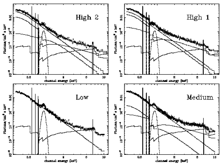
Figure 8: Unfolded EPIC-pn spectra for low, medium and both high-flux epochs during the low state. The various model components are plotted with lines. Note that power-law and absorbed Comptonised blackbody components do not contribute significantly to the low flux epoch spectrum.

5.3 Fit results

The best fitting model yields $\chi^{2}_{\nu}=1.37$ for 1159 d.o.f., for model parameters which are shown in Table 1. Data/model ratios are plotted in Fig. 7. Significant residuals still exist (see the Discussion for consideration of the causes of these residuals), although the model can reproduce the general spectral shape and variability reasonably well. Note that the apparent ‘absorption trough’ observed at $\sim 1.6$ keV in the second high flux epoch spectrum does not correspond to the probable weak systematic feature in the detector response observed at $\sim 1.8$ keV in the EPIC-pn spectrum of MCG–6-30-15 (, 2003). However, since this 1.6 keV feature in the EPIC-pn spectrum of NGC 4051 is not replicated in the EPIC-MOS spectra from this epoch it is likely to be a statistical artefact. Although the fit is not formally acceptable, the model appears to give a reasonable description of the overall spectral variability.

Figure 9: Unfolded model fit to the high1 spectrum. To make the contributions of the different continuum components clearer, they are plotted using thick lines. The absorbed and unabsorbed Comptonised blackbody components are plotted with a black dashed line and a solid grey line respectively. The reflection component and the absorbed pivoting power-law component are plotted with a solid black line and a black dotted line respectively.

To demonstrate the effects of the different model components on the spectral variability, we plot the unfolded models and spectra for the low, medium and both high flux epochs in Fig. 8. A more detailed plot of the unfolded model fit to the high1 spectrum is also shown in Fig. 9, with the various continuum components made more distinct to allow easier interpretation. We note that the model can explain the complicated spectral variability reported in Section 3 as being largely due to the variation of the hard and soft variable components relative to the constant components in the respective bands. In other words, the effect of power-law pivoting dominates the overall spectral variability of the source (i.e. across the entire observed flux range, as revealed in Fig. 4), but within the low state where the varying continuum flux is small, spectral variability due to the presence of constant components is much more important. For example, the hardening in response to small flux increases occurs when the soft variable thermal component is very weak compared to the constant soft component, so that the flux variation is primarily in the hard band, associated with the pivoting power-law (which though weak is still significant compared with the constant reflection component in that band). On the other hand, a large flux increase (e.g. the flare early in the observation) corresponds to the flux of the variable thermal component also increasing significantly, in addition to the hard power-law flux, so that the soft/hard flux ratio does not change. Note also that the divergence of the medium and high flux spectra below $\sim 5$ keV is explained by the model as being due to the larger Comptonised thermal component in the high flux spectrum. At the lowest fluxes the power-law contribution to the EPIC-pn spectrum is negligible, i.e. the spectrum is probably dominated by the constant thermal and reflection components.

Table 1: Best-fitting broadband model parameters.

	$\Gamma$	$A_{\rm cbb}$	$A_{\rm const}^{f}$	$kT_{\rm cbb}^{f}$	$kT_{\rm e}^{f}$	$\tau_{\rm cbb}^{f}$	$\tau_{\rm O{\sc vii}}^{f}$	$\tau_{\rm O{\sc viii}}^{f}$	$\tau_{\rm Fe}^{f}$	$R^{f}$
Low	-2.5	0.0	4.02	0.08	18.0	1.08	1.3	0.5	0.4	2.4
Medium	1.15	0.40	4.02	0.08	18.0	1.08	1.3	0.5	0.4	2.4
High 2	1.17	1.68	4.02	0.08	18.0	1.08	1.3	0.5	0.4	2.4
High 1	1.35	2.52	4.02	0.08	18.0	1.08	1.3	0.5	0.4	2.4

$\Gamma$ is the photon index of the pivoting power-law; $A_{\rm cbb}$ and $A_{\rm const}$ are the normalisations of the variable and constant Comptonised blackbodies respectively (units of $10^{4}$); $kT_{\rm cbb}$, $kT_{\rm e}$ and $\tau_{\rm cbb}$ are the blackbody temperature (in keV), and Comptonising electron temperature (in keV) and optical depth for the Comptonised blackbodies; $\tau_{\rm O{\sc vii}}$, $\tau_{\rm O{\sc viii}}$ and $\tau_{\rm Fe}$ are the edge optical depths and $R$ is the reflection scaling factor of the constant reflection component (see Section 6). Note that since the fit is not formally acceptable, meaningful errors cannot be quoted.
^f Values forced to be the same for all four spectra.

For completeness, we also substituted different soft spectral models for the constant and variable soft components used in the fit. Subsituting the Comptonised blackbody spectra with a diskpn model (, 1999) for a pure disk blackbody spectrum modified by a pseudo-Newtonian potential (to take account of relativistic effects), we obtain a much worse fit ($\chi^{2}_{\nu}=3.1$ for 1160 d.o.f.). If we instead substitute simple steep power-laws, the fit is poorer ($\chi^{2}_{\nu}=1.52$ for 1161 d.o.f., for photon index $\Gamma\simeq 3$) than obtained using Comptonised blackbodies, with the main residuals corresponding to a flattening of the observed spectrum below 0.5 keV. We conclude that, of the simple models tested here the Comptonised blackbody provides the best description of the soft component spectra (although see 2003, 2003 and Salvi et al., in prep., for an alternative description invoking a relativistic Oviii diskline and a steep power-law).

6 Discussion

We have demonstrated that the information gained from flux-flux plots can be used to infer the form of a spectral model which is relatively successful at replicating the seemingly complex X-ray spectral behaviour of NGC 4051 observed in the low state. Of course, significant residuals still remain in our model fits, and so our model should be considered only as an approximation to the true spectral behaviour. In this section, we will discuss some of the implications of our results and describe some of the practical and theoretical aspects of improving our model in relation to these implications.

6.1 The variable continuum components

The flux-binned 0.1-0.5 keV vs. 2-10 keV flux relation is well fitted by a power-law plus constant model, implying that the relation between these two bands, and the bulk of the spectral variability observed in NGC 4051 (over its entire flux range), is caused by the spectral pivoting of the power-law, also observed in the 2-15 keV band (, 2003). The presence of a constant-shape thermal component (which we model here with a Comptonised blackbody), which dominates the continuum at low energies, suggests that the pivoting power-law must be ‘attached’ to the thermal component, thus producing the observed flux-flux relation and the good correlation observed between extreme UV and medium energy X-ray fluxes (, 2000). An obvious physical realisation of this model is that the thermal component represents a directly observed variable source of seed-photons, which are upscattered in the corona to produce the variable power-law emission. In fact the observed blackbody temperature is close to the $\sim 0.1$ keV temperature expected from the small black hole mass of $\sim 3\times 10^{5}$ M_⊙, inferred for NGC 4051 from both reverberation mapping (, 2003) and the X-ray variability power spectrum (, 2003). The spectrum of NGC 4051 may then be unusual in this regard, since most AGN have larger black hole masses and hence their disk blackbody emission will not be directly observable in the soft X-ray band.

The fact that NGC 4051 appears to show a very strongly varying thermal component indicates a highly unstable accretion disk. Recent interpretations of AGN X-ray variability in terms of fluctuations in the accretion flow (implied by the observed ‘rms-flux’ relation and the similarity with X-ray binary systems, 2001, 2003) suggest that the accretion flow is geometrically thick, so that perturbations can propagate from a range of radii into the inner X-ray emitting regions. For AGN variability dominated by intrinsic variability of the power-law emission and not varying thermal emission, a geometrically thick but optically thin coronal accretion flow or advection dominated flow may suffice to explain the variability. However in the case of NGC 4051, where the thermal emission appears to drive the pivoting of the power-law (see below), the optically thick accretion disk must itself be geometrically thick in order for the model of propagating perturbations in the accretion flow to work (e.g. see Appendix to 2001). This situation can be realised at high accretion rates (e.g. 1992). The long-term average 2-10 keV X-ray luminosity of NGC 4051 from RXTE monitoring (e.g. 2003) of $\sim 3\times 10^{41}$ erg s^-1, corresponds to about 1% of the Eddington luminosity for the black hole mass given above. Depending on the assumed bolometric correction, the total luminosity is likely to be of the order of a few tens of % of Eddington, possibly sometimes reaching close to the Eddington rate, so a thick disk seems a likely configuration for the accretion flow in NGC 4051.

The physical connection between the thermal and power-law components will determine the shape of the spectrum in the intermediate energy range (perhaps 0.5-3 keV) where both components contribute significantly. For example, we might expect a rather smooth join between the components, with a shape determined by the underlying thermal spectrum and the temperature distribution of the Comptonising electrons, as well as other factors (e.g. geometry of the emitting regions). Therefore it is not surprising that our rather crude best-fitting model, which treats both components separately, is still not a very good fit to the data, especially in that intermediate energy range, where notable residuals can be seen. Additional complexities might exist, for example are there two populations of Comptonising electrons (as suggested by our model which includes both a hard pivoting power-law and a steeper Compton tail to the thermal component), or do the electron populations merge (e.g. as in a hybrid thermal-non-thermal plasma, 1999)? Spectral modelling with a more detailed theoretical underpinning may help answer these questions by providing much better fits to the data.

The pivoting power-law can be interpreted simply in terms of models where the luminosity of the X-ray emitting corona is constant and seed photons are varying (see 2002 and discussion in 2003). However, we note that there is intrinsic scatter in the unbinned flux-flux plots, implying an additional source of spectral variability which is independent of flux. We note that various spectral timing properties of NGC 4051 imply an additional variability process in the hard band which applies on short time-scales only (e.g. the flattening of the power spectrum at higher energies and the decrease in coherence between bands on short time-scales; 2003), which is likely to be the origin of much of the scatter in the HS flux-flux plot. (2003) suggested that the intrinsic scatter in the flux-flux plots may be due to weak variability of the hard component (possibly reflection) which is uncorrelated with the strongly variable power-law component. However, the fact that the scatter increases towards higher fluxes, as is shown in Appendix A, implies that the additional variable process is ‘aware’ of the large amplitude flux variability and hence is likely to be intrinsic to the variable power-law (note that this effect is related to the rms-flux relation observed in NGC 4051, 2003). Such additional variability in the power-law could arise from events which heat the corona on short-time-scales (e.g. magnetic flares) independent of the variations in seed photon flux which may be due to accretion instabilities.

6.2 Reflection, absorption and the nature of the constant continuum components

A strong reflection component (which we assume is constant) seems to be required to explain the data. The normalisation of the reflection component corresponds to a typical illuminating continuum 2-10 keV flux of $\sim 3\times 10^{-11}$ erg cm^-2 s^-1 for a reflector covering $2\pi$ steradian solid angle, as seen from the illuminating source (compare with the RXTE-observed average 2-10 keV flux since 1996 of $2.2\times 10^{-11}$ erg cm^-2 s^-1). One might assume therefore that the constant reflection could originate from a distant reflector. However, the reflection required to fit the 2002 low state spectrum is a factor$>2$ larger than than that used to explain the May 1998 spectrum observed by BeppoSAX and RXTE (, 1999), while the narrow 6.4 keV line flux is not larger than observed in May 1998, suggesting that a significant component of the reflection is not directly coupled to the narrow line flux and may not arise in a distant reprocessor. Furthermore, we point out that according to Fig. 1, at earlier epochs in the 2002 low state the 2-10 keV source flux dropped to significantly lower levels than we observed with XMM-Newton. Since our spectral fits suggest the source to be reflection dominated at the lowest fluxes observed by XMM-Newton, this suggests that the some significant fraction of the reflection component may itself vary on time-scales of weeks or less.

Weak variability of a reflection component, which is independent of the illuminating continuum flux is also implied by fitting a two-component model to data from MCG–6-30-15 (, 2003). Puzzlingly however, a diskline appears not to be required in NGC 4051, perhaps suggesting that more realistic models than we use here are required to explain the reflection, i.e. taking full account of relativistic smearing, disk ionisation or more complex reflection geometries (e.g. 2002). We note here that (2003) demonstrate in the specific case of NGC 4051 how strong, almost constant reflection can be produced by the effects of strong gravitational light bending on X-rays illuminating the disk from a source of variable height close to the black hole. (2003) point out that in low flux states (when the source is closest to the black hole, and hence light bending and relative reflection is most extreme), the inner disk is likely to be highly ionised, with attendant effects on the line strength and profile. Indeed the extreme variability of the thermal component in the spectrum of NGC 4051 (which may drive the spectral pivoting) further suggests that the inner accretion disk in NGC 4051 is very unstable, which may carry implications for the formation of prominent iron disklines.

We also detect a strong ($\tau\sim 0.4$) absorption edge at $\sim 7.9$ keV, possibly due to Fexvii. The presence of such a strong edge is puzzling, because it corresponds to an absorbing column of Fe $>10^{19}$ cm^-2, i.e. a hydrogen column $>10^{23}$ cm^-2 assuming Solar abundances. In the absence of a large overabundance of iron, it is difficult to imagine how such a large absorbing column could remain hidden at lower energies. This is because even if it is highly ionised (e.g. ionisation parameter $\xi\sim 10^{3}$–$10^{4}$), such a large column of gas would produce strong edges in lower-$Z$ elements which are not observed in the XMM-Newton grating spectrum of NGC 4051 in the normal state (, 2003). One cannot also simply argue that the column of gas in the line of sight is much larger in the low state, because the resulting discontinuity in the effects of absorption would not produce the gentle bending of the HS flux-flux relation between the normal and low state seen in Fig. 4. Note that these arguments appear to rule out the recent partial ionised absorber explanation for the spectral variability of NGC 4051 suggested by (2003), but these arguments also impose strong constraints on our interpretation of the edge at 7.9 keV detected in the low state. An alternative interpretation of the 7.9 keV edge is that it originates in reflection, rather than absorption, i.e. it may originate from the possibly constant reflection component. This interpretation would help to explain why this edge is not readily apparent in the normal state spectra (e.g. it is not reported by 2003), since it would be diluted by the higher continuum level in that state. Unfortunately, the spectra from different flux epochs within the low state do not have sufficient high energy signal-to-noise to test the flux dependence of the depth of the edge, but our hypothesis at least appears to be consistent with the lack of evidence for a very large column of absorbing gas at lower energies.

The presence of an absorption edge of Fexvii in reflection is consistent with a mildly ionised reflector with $\xi\sim 100$. Such a reflector would also produce edges of Ovii and Oviii and it is tempting to equate these features with the strong absorption edges ($\tau\sim 1$) we use to fit the low state data, which are required by the model in conjunction with a constant soft continuum component, in order to explain the lack of variability above $\sim 0.7$ keV and the resulting flattening of the MS flux-flux relation at low fluxes. In fact, one might explain both the soft absorption features and the constant soft component in terms of reflection of the primary continuum (in this case a Comptonised blackbody plus power-law), from different locations of an ionised disk. For example, if at low fluxes (where the constant, unabsorbed soft component dominates) only the innermost, heavily ionised regions of a disk are illuminated, then the reflected spectrum will be almost featureless and match closely the illuminating soft spectral shape. However, if the geometry of the source changes, so that at slightly higher fluxes the source height increases or the source becomes more vertically extended, the outer, less heavily ionised regions of the disk will also be illuminated and edges will be imprinted on the reflected spectrum. Or alternatively, at higher illuminating fluxes the outer disk may become sufficiently ionised to allow reflection in soft X-rays together with the accompanying edges, without requiring a change in source geometry. At even higher fluxes, those edges may be reduced by further ionisation (and hence do not appear in the normal state) or they may be diluted if the soft component of reflection somehow remains constant at higher fluxes, which is possible if the soft reflection has the same origin as the constant reflection component observed at harder energies. The basic physical picture we propose above to explain the constant soft component and possible edges may be consistent with the model of (2003), if it is extended to treat reflection from an ionised disk. However, it is unclear whether our interpretation that the variable thermal emission drives the power-law pivoting could apply in the model of (2003), since in that model the continuum variability is explained as being predominantly due to gravitational effects coupled with variations in height of a constant source.

An alternative explanation of the O edges (and/or possible Fe UTA) required by our model is that they represent simple absorption of the varying component of emission. In this case, the constant soft component is unabsorbed. This picture represents something like the partial covering scenario envisaged by (2003), albeit without the requirement of such a large column denisty of material, which seems problematic (as noted above). The optical depth of O edges required by our model correspond to ionic column densities of $\sim 10^{19}$ cm^-2 which are not easy to reconcile with the column densities observed in grating data of the normal state ($\sim 2\times 10^{17}$ cm^-2, 2003), even given a large drop in ionisation parameter. However the predicted total column in this case is $\sim 10^{22}$ cm^-2, lower than the value estimated by (2003), and may be consistent with the lack of strong edges observed at higher fluxes in the normal state. The requirement of only partial covering in this scenario remains difficult to explain however.

7 Conclusions

We have presented an analysis of EPIC-pn data from an XMM-Newton observation of NGC 4051 in the low state in 2002 November. We reach the following conclusions:

1. The spectral variability observed in NGC 4051 in the low state is complex (see Section 3). However, flux-flux plots show that the overall spectral shape in the low state is consistent with an extrapolation of the spectral pivoting of a power-law continuum observed at higher fluxes (Section 4), confirming the interpretation of earlier Chandra data by Uttley et al. (2003).

2. At softer energies, the variable spectrum is reasonably well described by a thermal component with a constant, Comptonised blackbody shape, which in order to explain the spectral variability, may be absorbed in the $\sim 0.7$–1 keV range, perhaps by photoelectric edges of Ovii/Oviii and/or unresolved transition arrays of Fe, which may possibly be associated with reflection features also seen at higher energies. The blackbody temperature ($kT\sim 0.1$ keV) of this Comptonised thermal component is consistent with the low black hole mass of NGC 4051 ($3\times 10^{5}$ M_⊙, 2003), and the strong variability of this component, correlated with the power-law pivoting at harder energies, suggest that it is the source of seed photons for the power-law continuum.

3. A constant reflection component and Fexvii edge can explain the hard spectral features (in addition to the pivoting power-law continuum), although a prominent diskline is not required. However, the apparent lack of long-term coupling between the reflection amplitude and the narrow iron line flux, together with the possible variability of the reflection component on time-scales of weeks suggest that some kind of disk reflection cannot be ruled out. The Fexvii edge requires an absorbing column of $N_{\rm H}>10^{23}$ cm^-2, but due to the lack of evidence for such a large absorbing column at lower energies we suggest the edge is observed in reflection.

4. A constant soft spectral component is also required to explain the spectral variability of NGC 4051. This constant soft component likely has a spectrum similar to that of the variable component, but without any absorption. The constant soft component might be related to the constant hard reflection component if the reflector is ionised, in which case a model similar to that of (2003) may help to explain the unusual spectral variability properties of NGC 4051 in the low state. Alternatively, partial covering of the emission by ionised gas of column density $\sim 10^{22}$ cm^-2 may explain the data.

Acknowledgments

We thank the anonymous referee for a number of helpful comments which improved this paper. This work was supported by grants from the UK Particle Physics and Astronomy Research Council (PPARC) including PPA/G/S/2000/00085. IM^cH also acknowledges the support of a PPARC Senior Research Fellowship. The work reported here is based on observations obtained with XMM-Newton, an ESA science mission with instruments and contributions directly funded by ESA Member States and the USA (NASA).

Appendix A Scatter in the HS flux-flux relation

Figure 10: Spread in the HS flux-flux relation (see Section 4 as a function of flux. The dotted line shows the 90% confidence upper limit in spread expected due to photon counting noise effects only, i.e. with no intrinsic scatter in the unbinned flux-flux relation (see text for details).

By assuming the best-fitting power-law plus constants model, we can determine the spread in data points around the binned HS flux-flux relation as a function of flux, and so confirm that the scatter does increase towards higher fluxes. We demonstrate this result in Fig. 10, which shows the rms spread in the flux bins used to plot the binned HS flux-flux relation. The spread in hard fluxes in a bin, $\sigma_{h}$ is determined using the equation:

$$\sigma_{h}=\sqrt{\frac{1}{n-1}\sum_{i=1}^{n}(H_{i}-h_{i})^{2}}$$ (2)

where there are $n$ individual hard-flux measurements ($h_{i}$) in the bin, and for each individual measurement $H_{i}$ is the hard-flux predicted from the observed soft flux by the best-fitting power-law plus constants model. Of course, some scatter in the relation can be caused by photon counting noise in both the hard and soft bands (which moves the data points on the flux-flux plot in vertical and horizontal directions respectively). The effect of this noise on the scatter is dependent on the form of the flux-flux relation and so is not a simple function of flux. For example, since the fitted flux-flux relation is a power-law with index$<1$, any scatter due to noise in the soft band is magnified at low fluxes, because the flux-flux relation is steeper, so that a horizontal shift in a data point at low fluxes will have a larger effect than the same shift at high fluxes. Therefore, to take account of the effects of photon counting noise, we used a simple bootstrap-type technique, assigning a hard flux value to each observed soft flux value using the best-fitting model for the binned HS flux-flux relation (i.e. assuming no intrinsic scatter) and then shifting each simulated data point in both the hard flux and soft flux directions by a zero-mean Gaussian deviate with standard deviation equal to the corresponding error bars, to produce a new realisation of the unbinned flux-flux plot. By simulating 1000 such realisations and measuring the scatter as a function of flux in each, we could estimate the distribution of the rms spread expected from photon counting noise only, in the absence of any intrinsic scatter. The resulting 90% confidence upper limit on the expected rms spread due to noise is shown as a dotted line in Fig. 10. Clearly the observed scatter and the increase in scatter with flux are highly significant.

References

- (1) Churazov E., Gilfanov M., Revnivtsev M., 2001, MNRAS, 321, 759
- (2) Collinge M. J., et al., 2001, ApJ, 557, 2
- (3) Elvis M., Lockman F. J., Wilkes B. J., 1989, AJ, 97, 777
- (4) Fabian A. C., Ballantyne D. R., Merloni A., Vaughan S., Iwasawa K., Boller Th., 2002, MNRAS, 331, L35
- (5) Fabian A. C., Vaughan S., 2003, MNRAS in press (astro-ph/0301588)
- (6) Frank J., King, A. R., Raine D. J., 1992, Accretion Power in Astrophysics. Cambridge Univ. Press, Cambridge
- (7) Gierlinski M., Zdziarski A. A., Poutanen J., Coppi P. S., Ebisawa K., Johnson W. N., 1999, MNRAS, 309, 496
- (8) Guainazzi M., Mihara T., Otani C., Matsuoka M., 1996, PASJ, 48, 781
- (9) Guainazzi M., et al., 1998, MNRAS, 301, L1
- (10) Lamer G., McHardy I. M., Uttley P., Jahoda K., 2003, MNRAS, 338, 323
- (11) Mason K. O., et al., 2002, ApJ, 580, L117
- (12) McHardy I. M., Papadakis I. E., Uttley P., Page M. J., Mason K. O., 2003, MNRAS submitted
- (13) Miniutti G., Fabian A. C., Goyder R., Lasenby A. N., 2003, MNRAS, 344, L22
- (14) Miniutti G., Fabian A. C., 2003, submitted to MNRAS (astro-ph/0309064)
- (15) Ogle P. M., Mason K. O., Page M. J., Salvi N. J., Cordova F. A., McHardy I. M., Priedhorsky W. C., 2003, ApJ, submitted
- (16) Pounds K. A., Reeves J. N., King A. R., Page K. L., 2003, MNRAS, submitted (astro-ph/0310257)
- (17) Salvi N. J., 2003, Ph.D. thesis, Univ. London
- (18) Shemmer O., Uttley P., Netzer H., McHardy I. M., 2003, MNRAS in press (astro-ph/0305129)
- (19) Shih D. C., Iwasawa K., Fabian A. C., 2002, MNRAS, 333, 687
- (20) Taylor R. D., Uttley P., McHardy I. M., 2003, MNRAS, 342, L31
- (21) Uttley P., McHardy I. M., Papadakis I. E., Guainazzi M., Fruscione A., 1999, MNRAS, 307, L6
- (22) Uttley P., McHardy I. M., Papadakis I. E., Cagnoni I., Fruscione A., 2000, MNRAS, 312, 880
- (23) Uttley P., McHardy I. M., 2001, MNRAS, 323, L26
- (24) Uttley P., Fruscione A., McHardy I., Lamer G., 2003, ApJ, 595, 656
- (25) Uttley P., 2003, submitted to MNRAS
- (26) Zdziarski A. A., Poutanen J., Paciesas W. S., Wen L., 2002, ApJ, 578, 357