Convection in the atmospheres and envelopes of Pre-Main Sequence stars

The ${T}_{\rm eff}$ location of Pre-Main Sequence (PMS) evolutionary tracks depends on the treatment of over-adiabaticity (D’Antona & Mazzitelli 1994, 1998). Since the convection penetrates into the stellar atmosphere, also the treatment of convection in the modeling of stellar atmospheres will affect the location of the Hayashi tracks. In this paper we present new non-grey PMS tracks for $\mbox{${T}_{\rm eff}$}>4000$ K. We compute several grids of evolutionary tracks varying: i) the treatment of convection: either the Mixing Length Theory (MLT) or Canuto et al. (1996, CGM) formulation of a Full Spectrum of Turbulence; ii) the atmospheric boundary conditions: we use the new Vienna grids of ATLAS9 atmospheres (Heiter et al. 2002a), which were computed using either MLT (with $\alpha=\Lambda/H_{\rm p}=0.5$) or CGM treatments. For comparison, we compute as well grids of models with the NextGen (Allard & Hauschildt 1997, AH97) atmosphere models, and a 1 ${\rm M}_{\odot}$ grey MLT evolutionary track using the $\alpha$ calibration based on 2D-hydrodynamical models (Ludwig et al. 1999). These different grids of models allow us to analyze the effects of convection modeling on the non–grey PMS evolutionary tracks. We disentangle the effect on a self-consistent treatment of convection in the atmosphere of the wavelength dependent opacity, from the role of the convection model itself in the atmosphere and in the interior. We conclude that: i) In spite of the solar calibration, if MLT convection is adopted a large uncertainty results in the shape and location of PMS tracks, and the MLT calibration loses sense. ii) As long as the model of convection is not the same in the interior and in the atmosphere, the optical depth at which we take the boundary conditions is an additional parameter of the models. iii) Furthermore, very different sub-atmospheric structures are obtained (for MS and PMS stellar models) depending not only on the treatment of convection, but also on the optical depth at which the boundary conditions are taken. iv) The comparison between NextGen based models and ATLAS9 based models shows that in the ${T}_{\rm eff}$ domain they have in common (4000–10000K) the improved opacities in NextGen atmosphere models have no relevant role on the PMS location, this one being determined mainly by the treatment of the over-adiabatic convection. v) The comparison between theoretical models and observational data in very young binary systems indicates that, for both treatments of convection (MLT and CGM) and for any of the atmosphere grids (including those based on the 2D-hydrodynamical atmosphere models), the same assumption for convection cannot be used in PMS and MS: either the models fit the MS – and the Sun in particular– or they fit the PMS. Convection in the PMS phase appears to be less efficient than what is necessary in order to fit the Sun.

1 Introduction

The experimental data presently available for young objects in star-formation regions need to be compared with theoretical evolutionary tracks in order to be correctly interpreted in terms of age, mass and chemical composition. As discussed in D’Antona (2000) and the references therein, the HR diagram location of a star during its Pre-Main-Sequence (PMS) evolution is very sensitive to physical inputs such as low–temperature opacity, equation of state, rotation, atmosphere model, and convection treatment.

During the last years, a lot of work has been done to improve the knowledge of low–temperature opacities and to include them in the modeling of stellar atmospheres. The variety of theoretical evolutionary tracks available today (new convection treatment with grey boundary conditions; classic convection with non–grey atmosphere models…) has contributed to create some confusion about the effect of the different physical inputs on the results. Our aim is to extricate the different roles of non–grey atmospheres and of convection in evolutionary track computations. As shown by Montalbán et al. (2001), that can be done only using models with a self–consistent treatment of convection both in the atmosphere and in the interior.

In stars on the cool side of the HR diagram, convection is deep and defines the “envelope” portion of the star in which the dominant mode of energy transport is convection. In particular, Pre–Main Sequence (PMS) models are largely convective and — due to the low gravity and low temperature — the convection can be over–adiabatic in extended regions of the stars. Consequently, the shape of the corresponding evolutionary tracks depends on the efficiency of the convective transport of energy.

The convective zone increases with decreasing ${T}_{\rm eff}$  and it is gradually shifted towards larger depths, so that the structure of the surface layers is less and less affected by the convection as ${T}_{\rm eff}$ decreases. For temperatures lower than 4700K, however, the convection zone rises again due to the dissociation of ${\rm H}_{2}$. On the other hand, for given ${T}_{\rm eff}$ and metallicity, and decreasing gravity, the convective flux decreases because of the lower density and, therefore, the over-adiabatic region in the atmosphere is more extended. Consequently, in cool stars, a large part of the photosphere actually forms the uppermost portion of the convective envelope.

Several facts indicate that the classical grey atmosphere approximation adopted in stellar computation is not valid for cool stars: the diffusion approximation is not valid up to $\tau=2/3$ (Morel et al. 1994), and the convective transport of energy has to be taken into account in the atmosphere as well. Furthermore, the introduction of the frequency dependence of opacity modifies the onset of convection, and the grey approximation produces errors in the theoretical ${T}_{\rm eff}$  and in the colors of low mass stars (Baraffe et al. 1995; Baraffe & Chabrier 1997). Therefore, in the computation of stellar models, the boundary conditions (BCs) at the surface must be provided by non–grey modeling of stellar atmospheres, taking into account the dependence of opacity on frequency and an adequate treatment of convection.

Unfortunately, for the time being, only very simple local convection models are available for routine computation of extended grids of model atmospheres, while detailed numerical simulations are still unaffordable for applications such as stellar evolution that requires the calculation of many thousands of individual model atmospheres over the HR diagram.

The “standard model” of convection in stellar evolution is the mixing length theory (MLT, Böhm–Vitense 1958), where turbulence is described by a relatively simple model that contains essentially one adjustable parameter, the mixing length: $\Lambda=\alpha H_{\rm p}$ ($H_{\rm p}$ being the local pressure scale height and $\alpha$ an unconstrained parameter). Canuto & Mazzitelli (1991, CM) and Canuto et al. (1996, CGM) made available an alternative model (Full Spectrum Turbulence –FST– models), that overcomes some of the problems of MLT, while keeping a low computational cost. The main characteristics and differences of these models are described in Sect 2.

D’Antona & Mazzitelli (1994, DM94) published four sets of PMS evolutionary tracks that allowed to study the effect of low-temperature opacity and treatment of convection on stellar evolution. These tracks were computed with both kinds of convection treatments: MLT calibrated on the Sun, and the FST model with the CM formalism. The results showed that the ${T}_{\rm eff}$ location of Hayashi tracks has a strong dependence on the treatment of convection. DM94’s models, widely used and tested with observations, were revised in D’Antona & Mazzitelli (1997, 1998 — DM97, 98) by introducing several improvements in the micro–physics (updated opacity tables and equation of state) and in the macro–physics (the updated FST treatment of convection by Canuto et al. 1996). The DM97 models were still employing grey atmospheric BCs, but the problem of matching convection in the interior and in the atmosphere occurs already in these models. In fact the DM97,98 models make only an exploratory approximation for defining the convective scale length if convection penetrates in the atmosphere, namely, they do not include the atmospheric convective depth in the computation of the scale. With this choice, convection in the sub–photospheric layers is less efficient, and very low mass stars are cooler by up to $\sim 150$ K. DM98 suggested that since the over–adiabaticity is present in low gravity / low temperature atmospheres, the FST convection treatment would modify convection also in the atmosphere, therefore it would be very important to include a revised treatment of convection in model atmospheres.

Recently, Heiter et al. (2002a) have published new atmosphere model grids based on Kurucz’s ATLAS9 code (1993). They performed calculations for different treatments of non–adiabatic convection: MLT ($\alpha=0.5$), CM, and CGM (for a smaller range of parameters, MLT —  $\alpha=1.25$ — was used as well). These choices for modeling convection are extensively motivated in Sect. 2 of that paper. As one of their main results, the authors conclude that MLT models with a small mixing length parameter (e.g., $\alpha\sim 0.5$) and FST models are equivalent in the atmospheric region where the observed flux originates. Both treatments predict a low convective efficiency for these layers. The deep atmospheric structures, however, are different, and each $T(\tau)$ relation represents stars which differ in radius and luminosity, hence the PMS tracks will also be different. Furthermore, if MLT is adopted, and a low $\alpha$–value is used in the atmosphere ($\alpha_{\rm atm}$) ($\alpha_{\rm atm}$=0.5, as adopted in Heiter et al. 2002a, or $\alpha_{\rm atm}$=1 as in Hauschildt et al. 1999a), we must compensate, in order to fit the Sun, for the high over-adiabaticity in the atmosphere, by using an $\alpha$-value in the interior ($\alpha_{\rm int}$ much larger than $\alpha_{\rm atm})$. FST, by construction, reproduces this behavior: it is very inefficient at the outer boundary of the convection zone, and very efficient in the inner layers. As a consequence, FST has the advantage of simultaneously (and thus consistently) fitting, without arbitrary tuning of the parameter set ($\alpha_{\rm atm},\tau_{\rm ph},\alpha_{\rm int}$), the Balmer line profiles (Heiter et al. 2002a) and the solar radius (Heiter et al. 2002b and this paper).

In order to analyze the impact of sub–photospheric convection on the HR location of the Hayashi tracks, we computed solar composition stellar models for masses from 0.6 to 2.0 ${\rm M}_{\odot}$ with several combinations of convection model and boundary conditions (Table 1). The physical inputs of these models are described in Sect. 3.

An additional problem to be considered when computing stellar models with non–grey boundary conditions is the choice of $\tau_{\rm ph}$. From this point, the integration of the atmospheric stratification supplies the values of ${T}_{\rm eff}$ and ${\log g}$ (or luminosity and radius) for a given mass. If the atmospheric integration is consistent with the physics in the interior, and the diffusion approximation holds below $\tau_{\rm ph}$, the model location in the HR diagram should not depend on the choice of $\tau_{\rm ph}$. Since grids of atmosphere models and interiors are usually computed by different teams with different aims, quite often the physics (convection model, opacity, equation of state, etc.) used in both regions is not exactly the same. In Sect. 4 we analyze how these differences affect the evolution and structure of 1 ${\rm M}_{\odot}$ star.

In Sect. 5 we present our new non-grey PMS evolutionary tracks for ${T}_{\rm eff}$ $\geq 4000$ K. We have also computed two grids of “complete” FST models with metallicity larger and smaller than the solar one by a factor of 2. The effect of different chemical compositions on HR diagram location is shown in Sect. 6.

In Sect. 7 we compare our new FST Hayashi tracks with the available data for young binary stars in star-formation regions. In fact, PMS binaries having experimentally known masses are the best test for the PMS models, since they should fit both masses and display the same age. Finally, the main conclusions of this paper are summarized in Sect. 8.

2 About convection in stellar modeling

The system of equations describing stellar convection from first principles is both non–linear and non–local and its analytical or numerical solution for the general stellar case is not yet available. Even numerical simulations not resolving all the spatial scales of the flow are unaffordable for stellar evolution modeling, at least for the intermediate future, because of the excessive thermal relaxation time scales of stellar structure modeling. Non–local models such as those proposed by Xiong (1985), Canuto (1992), and Grossman (1996) are a promising and much more affordable alternative with the present computational resources. But for the time being, in stellar modeling we still stick to local models: the “standard” Mixing Length Theory (Böhm–Vitense 1958), and the “Full Spectrum of Turbulence” formalisms (Canuto & Mazzitelli, 1991; Canuto et al. 1996) are two examples.

MLT treats the heat transport with a one-eddy incompressible model with compressibility partially accounted for through the definition of a mixing length $\Lambda=\alpha\,H_{\rm p}$, where $H_{\rm p}$ is the local pressure scale height and $\alpha$ is a free parameter. Mimicking the spectral distribution of eddies by one “average” eddy (reliable only for high viscosity fluids) has critical consequences on the computation of MLT fluxes: Canuto (1996) showed that in the limit of highly efficient convection ($S\gg 1$, where $S$ is the convective efficiency, see e.g. CM for details) MLT underestimates the convective flux (a fact also confirmed by laboratory data, Castaing et al. 1989), and in the low efficiency limit ($S\ll 1$) MLT overestimates the convective flux.

Computations show that inside the stars with deep convective regions $S\ll 1$ at the top of the convective envelope, just below the surface, while at the peak of the super-adiabaticity $S\gg 1$. In inefficient convection, the convective temperature gradient sticks to the radiative one and begins detaching from it only when convection becomes efficient.

Historically, the choice of a mixing length $\Lambda=\alpha\,H_{\rm p}$ is in part a consequence of this underestimation of fluxes in MLT. Thus, the scale length $\Lambda$ was originally (Böhm & Stückl 1967) chosen coincident with the distance $z$ from the convective boundary, consistently with the Von Karman law for incompressible fluids (Prandtl 1925), but due to the underestimation of convective flux, models with $\Lambda=z$ were not able to fit the Sun. Then, $\Lambda=\alpha\,H_{\rm p}$ grew up as standard choice, with the free parameter $\alpha$ calibrated by comparing the solar models with the actual Sun. Depending on the physical inputs the value of $\alpha$ can vary in between 1.5 and 2.2. If we use this prescription for the mixing length, at the peak of the super-adiabaticity, $\alpha\,H_{\rm p}\gg z$, and the fluxes, which are $\propto\Lambda^{2}$, are artificially increased.

FST (CM and CGM) models attempt to overcome the one–eddy approximation by using a turbulence model to compute the full spectrum of a turbulent convective flow. The treatment of turbulence in CM and CGM is slightly different. Nevertheless, in both cases the derived convective fluxes are quite distinct from the MLT ones. CM and CGM convective fluxes are $\sim 10$ times larger than the MLT ones for the $S\gg 1$ limit while, for the low efficiency limit ($S\ll 1$), the CM flux is $\sim 1/10$ of the MLT flux, and the CGM one $\sim 0.3$ times the MLT flux. This behavior yields, in the over-adiabatic region at the top of a convection zone, steeper temperature gradients for FST than for solar–tuned MLT (and, in the FST framework, gradients steeper for CM than for CGM).

Like MLT, FST models assume the Boussinesq approximation. Following the physical argument that the Boussinesq approximation leaves no natural unit of length other than the distance to a boundary ($z$) and the vertical stacking of the eddies due to density stratification, CM and CGM adopt respectively $\Lambda_{\rm CM}=z$, and $\Lambda_{\rm CGM}=z+\alpha^{*}H_{\rm p,top}$. The second term in $\Lambda_{\rm CGM}$ is a fine tuning parameter that allows small adjustments, if exact stellar radii are needed, e.g., in helioseismology. Canuto et al. (1996) stress however, that the role of $\alpha^{*}$ in FST models is radically different from that of $\alpha$ in the MLT model. FST tuning affects, in fact, only layers close to the boundaries since, for inner layers, $z$ quickly grows and becomes much larger than $\alpha^{*}H_{\rm p,top}$. On the other hand, if we wish to attribute a physical meaning to $\alpha^{*}$, the second term in $\Lambda_{\rm CGM}$ can be interpreted as an “overshooting term” representing the observed fact that convection penetrates in the stable region, and thus the scale length cannot decay to zero right at the depth where $\nabla_{\rm rad}=\nabla_{\rm ad}$ (Schwarzschild criterion of stability). In any case, $\alpha^{*}$ in these models is not properly used as an overshooting parameter but only to define the exact scale length.

The FST fluxes have also been used combined with other definitions of the mixing length. Bernkopf (1998), for instance, uses the CM version of the FST fluxes combined with a mixing length $\Lambda=\alpha H_{p}$ and with $\alpha<1$.

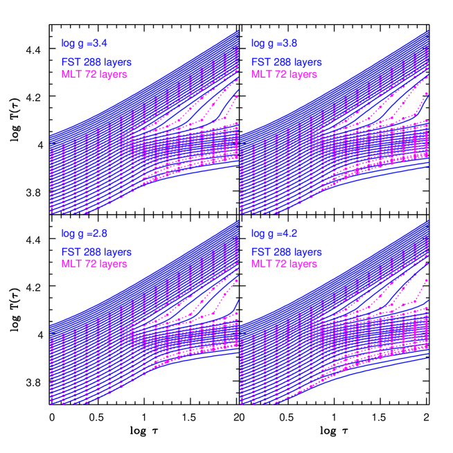
Figure 1: $T(\tau)$ relations computed using ATLAS9, a FST treatment of convection with $\alpha^{*}=0.09$ (Heiter et al. 2002a) and integrated using 288 layers (solid lines), or a MLT one with $\alpha=0.5$ and 72 layers (dotted lines and full circles). The lower curves correspond to ${T}_{\rm eff}$=4000 K and the upper curves to ${T}_{\rm eff}$=10000 K, with a step $\Delta$${T}_{\rm eff}$=200 K.

3 The stellar models

The stellar models presented here were computed using the stellar evolution code ATON2.0 (Ventura et al. 1998a). Specific details concerning the computation of the pre–main sequence and deuterium burning phases are described in Mazzitelli & Moretti (1980). We computed models for three metallicities $[M/H]=-0.3,0.0,$ and +0.3 with an adopted helium mass fraction $Y=0.28$. Three different sets of boundary conditions were considered for solar composition: two of the new grids of ATLAS9 atmospheres from Heiter et al. (2002a), MLT ($\alpha=0.5$) and CGM grids, and, for comparison, the non–grey atmosphere models by AH97. In the first case the considered masses span the interval 0.6 to 2.0 ${\rm M}_{\odot}$, in the second one that from 0.6 to 1.5 ${\rm M}_{\odot}$. For the other two chemical compositions only CGM models were computed. In addition, we computed a grey MLT evolutionary track for 1 ${\rm M}_{\odot}$ using for $\alpha$ the values provided by the calibration from 2D-hydrodynamical atmosphere models (Ludwig et al. 1999).

3.1 Equation of state and opacities

A complete description of the equation of state (EOS) of our code is given in Montalbán et al. (2000). For the present models, the thermodynamics is from Rogers et al. (1996), for five different hydrogen abundances. At temperatures $T\geq$ 6000 K we adopt the OPAL radiative opacities ($\overline{\kappa}$) (Roger & Iglesias 1996, for the solar Z–distribution from Grevesse & Noels 1993). In the high–density ($\rho$) regions the opacities are linearly extrapolated ($\log\leavevmode\nobreak\ \overline{\kappa}\,\,vs.\log\leavevmode\nobreak\ \rho$), and harmonically added to conductive opacities by Itoh & Kohyama (1993). At lower temperatures we use the Alexander & Ferguson’s (1994) molecular opacities (plus electron conduction in full ionization) for the same H/He ratios as in the OPAL case.

3.2 Atmospheric structure and boundary conditions

The new grids of ATLAS9 atmospheres by Heiter et al. (2002a) introduced several improvements in comparison with previous model grids published by Kurucz (1993, 1998) and Castelli et al. (1997). Most of them are related to a finer grid spacing ($\Delta$${T}_{\rm eff}$, $\Delta\log g$, but also vertical resolution) which allows a more accurate interpolation within the grids. For the convenience of the reader we recall the main characteristics of these grids:

• Three different models of convection: MLT($\alpha=0.5$), FST according to CM, and FST CGM.

• For FST models, an increase of the vertical resolution in the atmospheric integration from 72 to 288 layers ranging from $\log\tau_{\rm Ross}=-6.875$ to $\log\tau_{\rm Ross}=2.094$ (where $\tau_{\rm Ross}$ is the average Rosseland optical depth).

• Effective temperature range: 4000–10000 K, with $\Delta$${T}_{\rm eff}$ = 200 K.

• Gravity range: $\log g$ from 2.0 to 5.0, with $\Delta\log g=0.2$.

• Chemical composition: sets for [M/H]=–2.0, –1.5, –1.0, –0.5, –0.3, –0.2, –0.1, 0.0, +0.1, +0.2, +0.3, +0.5, +1.0 are available.

From the atmosphere models we built the tables of BCs corresponding to a fixed $\tau_{\rm ph}$. These tables contain, for each (${T}_{\rm eff}$,${\log g}$,[$M/H$]), the following quantities: temperature $T$($\tau_{\rm ph}$), pressure $P$($\tau_{\rm ph}$), geometrical depth $z$($\tau_{\rm ph}$), geometrical depth $z(\tau_{0})$ at the optical depth $\tau_{0}$ for which $\nabla_{\rm rad}=\nabla_{\rm ad}$, and finally the pressure scale height $H_{\rm p}(\tau_{0})\equiv H_{\rm p,top}$. We built tables corresponding to $\tau_{\rm ph}$=1, 3, 10, and 100 in order to analyze the dependence of the results on $\tau_{\rm ph}$. We note, however, that Heiter et al. (2002a) advise to switch between model atmosphere and stellar envelope at $\tau_{\rm ph}$=10, to avoid the discrepancies due to the turbulent pressure not included in the atmosphere modeling and to reduce the effect of different opacity tables and equation of state used at both sides of $\tau_{\rm ph}$. The boundary conditions for the internal structure are determined by spline interpolation of these tables. From the initial ${T}_{\rm eff}$ and $\log L$ we determine $P$ and $T$ at the last point of the internal structure ($\tau_{\rm ph}$) and the derivative of $P$ and $T$ with respect to luminosity and radius. An iterative procedure is performed until the $P(\tau_{\rm ph})$ and $T(\tau_{\rm ph})$ values derived at the boundary $\tau_{\rm ph}$ from the interior or from the atmosphere models converge. In order to take into account the effect of the penetration of convection into the atmosphere, the thickness of the convection zone in the atmosphere is included in the definition of the scale length $\Lambda$ in the FST models (see the discussion of Eq. (3.3) below).

Some parts of the tracks for 0.6 and 0.7 ${\rm M}_{\odot}$ reach ${T}_{\rm eff}$ $<4000$ K, falling outside the grid of ATLAS9 models. We completed the evolution by assuming as boundary conditions the values of $P$ and $T$ for the 4000 K grid points. The track is then artificial until ${T}_{\rm eff}$ becomes again larger than $4000$ K, but this does not introduce large errors in the determination of the following evolution to the MS. We recall here that the validity of the plane parallel approximation for $\log g\geq 2$, and for the ${T}_{\rm eff}$ domain of interest for our work, has already been shown by Hauschildt et al. (1999b) and Baraffe et al. (2002) for the case of NextGen model atmospheres. We can hence safely to assume its validity for the ATLAS9 model atmospheres as well.

Concerning the NextGen model atmospheres (AH97), their opacities include the contribution of many more molecular lines than the ATLAS9 ones, consequently, they are more adequate to study the ${T}_{\rm eff}$ region where these opacities dominate (roughly, below 4000 K). In AH97 models, the convection is treated with MLT and $\alpha=1$. For solar metallicity, the available models have ${T}_{\rm eff}$ from 3000 to 10000 K, and a surface gravity from $\log g=3.5$ to 6.0, with $\Delta\log g=0.5$; the vertical resolution in the atmospheric integration is of 50 layers ranging from $\tau=10^{-7}$ to 100 (only 9 layers between $\tau=1$ and 100).

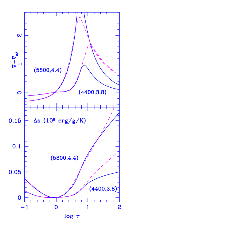
Figure 2: Upper panel: over-adiabaticity as a function of the optical depth in the atmosphere for two pairs of (${T}_{\rm eff}$,${\log g}$) corresponding to typical values for a 1 ${\rm M}_{\odot}$ star during MS and PMS. Dashed lines correspond to MLT ATLAS9 ($\alpha_{\rm atm}=0.5$) atmosphere models, and solid lines to CGM FST ones. Lower panel: Entropy jump for the same atmospheres as in upper panel.

3.2.1 The treatment of convection in the atmosphere

The original ATLAS9 code treats the convection by using MLT with $\alpha=1.25$  (cf. Castelli et al. 1997). In addition, the code has the possibility of including a sort of “overshooting”. The value $\alpha$=1.25 and the option of approximate overshooting were originally adopted to fit the intensity spectrum at the center of the solar disk and the solar irradiance. However, Castelli et al. (1997) showed that these quantities are much more sensitive to the overshooting–on mode than to the value of $\alpha$ itself (see also Heiter et al. 2002a) and that, if this treatment is included, the H_α and H_β profiles of the solar spectrum cannot be simultaneously matched. Several papers on: i) the ${T}_{\rm eff}$ determination from H_α and H_β lines (e.g., Fuhrmann et al. 1993, 1994; Van’t Veer–Menneret & Megessier 1996; Van’t Veer-Meneret et al. 1998); ii) the theoretical predictions of H_α and H_β (Gardiner et al. 1999 from 1D models, and Steffen & Ludwig 1997 from 2D numerical simulations), of $(b-y)$ and $c$ Strömgren indices (Smalley & Kupka 1999) and of Geneva indices (Schmidt 1999), and iii) abundance determinations (Heiter et al. 1998), indicate that, even if a 1D–homogeneous model cannot explain all the spectroscopic and photometric observations, atmosphere models predicting temperature gradients closer to the radiative one (i.e., those models in which convection is less efficient than predicted by MLT–based models with $\alpha>1$) are in better overall agreement with observations. As pointed out, however, in the above–mentioned papers, not all the color indices over the whole ${T}_{\rm eff}$ domain can be reproduced with such models either. Whereas in other cases, the quality of a fit (such as line profiles of H_α) is even independent of any sensible value of $\alpha$ (although not of other modifications to the convection treatment such as “approximate overshooting”).

In the new ATLAS9-MLT grids, the convection is described as in Castelli (1996) and Castelli et al. (1997) (that is $V/A=\Lambda/6$ and $y=0.5$), but with $\alpha=0.5$  and without “overshooting”. In the CGM model atmospheres, the convective flux is computed as in Canuto et al. (1996), but the characteristic scale length is defined as: $\Lambda=\min(z_{\rm top}+\alpha^{*}H_{\rm p,top},z_{\rm bot}+\alpha^{*}H_{\rm p,bot})$ where the index “top” and “bot” refers to top and bottom of the convective region. For most model atmospheres the difference with respect to the original prescription in Canuto et al. (1996) is either null or negligibly small, because the temperature gradient for convection zones which are entirely contained within the atmosphere is practically the radiative one, while, for convection zones extending below the atmosphere, the evaluation of $\Lambda$ in a pure model atmosphere has necessarily to occur near the top of the convection zone (Heiter et al. 2002a).

Since the effect of varying the fine tuning parameter $\alpha^{*}$ is felt only in a small region close to the boundary of the convection zone, changing $\alpha^{*}$ – say – by a factor two yields no difference in the solar spectrum features, so that its value cannot be calibrated from atmosphere models. Therefore, the choice of a value of $\alpha^{*}=0.09$ was based on the solar calibration performed by Canuto et al. (1996), but it has to be pointed out that this value was determined using grey BCs (Henyey et al. 1965).

As shown in Heiter et al. (2002a) the temperature structure in the deep atmosphere is strongly dependent on the convection model (Fig. 1). Because of the features of convective fluxes described in Sect. 2, the convection modeled with MLT ($\alpha=0.5$) is very inefficient in the whole atmosphere, while the FST models, which are similarly inefficient at the outer boundary, rapidly begin to be very efficient in the deeper layers of solar-like convection zone. In Fig. 2 we plot the over-adiabaticity and the jump of specific entropy corresponding to either MLT or FST atmosphere models with two different values of ${T}_{\rm eff}$ and ${\log g}$. The stellar spectra are not sensitive to the deep atmosphere gradients, and from the point of view of atmosphere models, as long as one uses a low value of $\alpha$, MLT and FST are essentially equivalent. The BCs provided by both atmosphere models can become, however, very different as the optical depth where the BCs are taken increases.

3.2.2 Resolution

Schmidt (1999) showed that a scale length prescription as used in CM or CGM together with a low vertical resolution could result in “jumps” in the grids of $\max(F_{\rm conv}/F_{\rm tot})$ as function of ${T}_{\rm eff}$/${\log g}$. That is due to the fact that the convective zone expands in total size and retreats from the upper/mid photosphere when going from high–${T}_{\rm eff}$/low–$g$ to low–${T}_{\rm eff}$/high–$g$. A change of the vertical extension of the convective zone even of a single layer can have a significant impact on the value of $\Lambda(z)$, and hence on $F_{\rm conv}$ ($\sim\Lambda^{8}$ in the low efficiency regime, see Gough & Weiss 1976 and references therein). Another aspect of the same problem was detected in computing FST stellar models with 72–layers atmosphere models as BCs. The thickness of the convection zone in the atmosphere $\Lambda_{\rm atm}=z(F_{\rm conv}=0)-z(\tau=\tau_{\rm ph})$ as a function of ${\log g}$ and ${T}_{\rm eff}$ was far from being smooth, in particular in the low–${T}_{\rm eff}$/low–$g$ region of the HR diagram, where convection quickly extends into the higher atmosphere layers due to the contribution of H^- and H₂ to the opacity. So, the resulting evolutionary paths in the HR diagram showed oscillations which disappear when new models with 288 layers are used.

The comparison between the $T(\tau)$’s relations for CGM-atmosphere models integrated with 72 and with 288 layers (see Fig. 1 in Montalbán et al. 2002) illustrates a result which from a different point of view was also discussed by Heiter et al. (2002a): in the case of ionization regions it is possible to correctly follow the rapid increase of temperature only if the number of layers is large enough. The same figure also points out a large uncertainty introduced for F and G stars (depending on their surface gravity), when the boundary condition is taken at optical depths $\tau_{\rm ph}$ larger than 20, because of the onset of (nearly) adiabatic convection in the envelope of cool stars compared to the (almost) radiative temperature gradient of hotter stars.

Atmosphere models are usually built to generate synthetic spectra to be compared with the observations. As a consequence, the number of mesh points per unit optical depth must be kept large in the region where the continuum and the lines are formed, that is at low optical depth, while few points are computed in between $\tau=10$ and $\tau=100$, though this is the recommended region (Morel et al. 1994) to adopt the values of temperature and pressure as BCs for the internal structure computation. The differences between $T(\tau)$’s relations corresponding to 72-CGM and 288-CGM atmosphere models show that low resolution models could induce non–negligible errors in the BCs, especially if $\tau_{\rm ph}$=100 is chosen as match point between the atmosphere and the interior.

3.3 Convection modeling in the interior

For the interior as well, models are computed either by MLT or FST. If we want to build complete stellar models using the MLT treatment of convection and fit the Sun, we should use $\alpha$–values in the interior ($\alpha_{\rm int}$) much larger than that one in the atmosphere ($\alpha_{\rm atm}=0.5$) (see Sect. 4).

The MLT used in the interior strictly follows the formulation of Cox & Giuli (1968), who chose the $V/A$ relation in order to obtain numerical agreement with the results of Böhm–Vitense (1958). In the atmosphere, as mentioned above, the MLT formulation follows Castelli (1996). There, the choice of $y$ and $V/A$ parameters is such that for the same $\alpha$–value, the efficiencies of convection in Cox & Giuli formulation ($\Gamma_{\rm CG}$) and in Castelli ($\Gamma_{\rm C}$) hold the relation $\Gamma_{\rm CG}=2/3\Gamma_{\rm C}$. This difference is much smaller than that introduced in the efficiency of convection by varying the $\alpha$–value from –say– 1.7 to 0.5.

The FST model of convection adopts the CGM fluxes, and the scale length at the radial coordinate $r$  is the harmonic average between $z_{\rm top}$ (distance to the top of convection increased by $\alpha^{*}H_{\rm p,top}$) and $z_{\rm bot}$ (distance to the bottom of convection increased by $\alpha^{*}H_{\rm p,bot}$), namely

$$\Lambda=z_{\rm top}\,z_{\rm bot}/(z_{\rm top}+z_{\rm bot})$$

This choice ensures that, close to the boundaries, $z\sim z_{\rm top}$ or $z\sim z_{\rm bot}$, and, far from boundaries, $\Lambda\sim H_{\rm p}$, as it should be expected (for details see Ventura et al. 1998a). For the models in which convection penetrates in the atmosphere, the quantity $z_{\rm top}$ has to include the distance from the bottom of the atmosphere ($z(\tau_{\rm ph})$) to the top of convection in the atmosphere ($z(\tau_{0})$), and $H_{\rm p,top}$ is also evaluated at $z(\tau_{0})$ in the atmosphere. So,

$$z_{\rm top}(r)=[z(\tau_{0})-z(\tau_{\rm ph})]+(R_{\rm max}-r)+\alpha^{*}H_{\rm p}(\tau_{0}),$$

where $r$  is the radius of the layer and $R_{\rm max}$ is the radius of the last point computed by the integration from the interior, that is the radius of the boundary point ($\tau_{\rm ph}$).

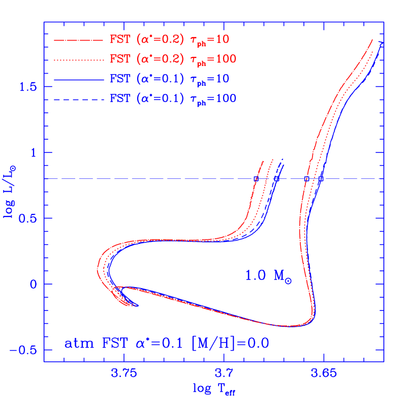
Figure 3: FST evolutionary tracks for 1 ${\rm M}_{\odot}$ for two different choices of the tuning parameter $\alpha^{*}$ and two different choices of the sub-photospheric boundary, $\tau_{\rm ph}$=10 and 100. The horizontal line refers to the models in Fig. 4

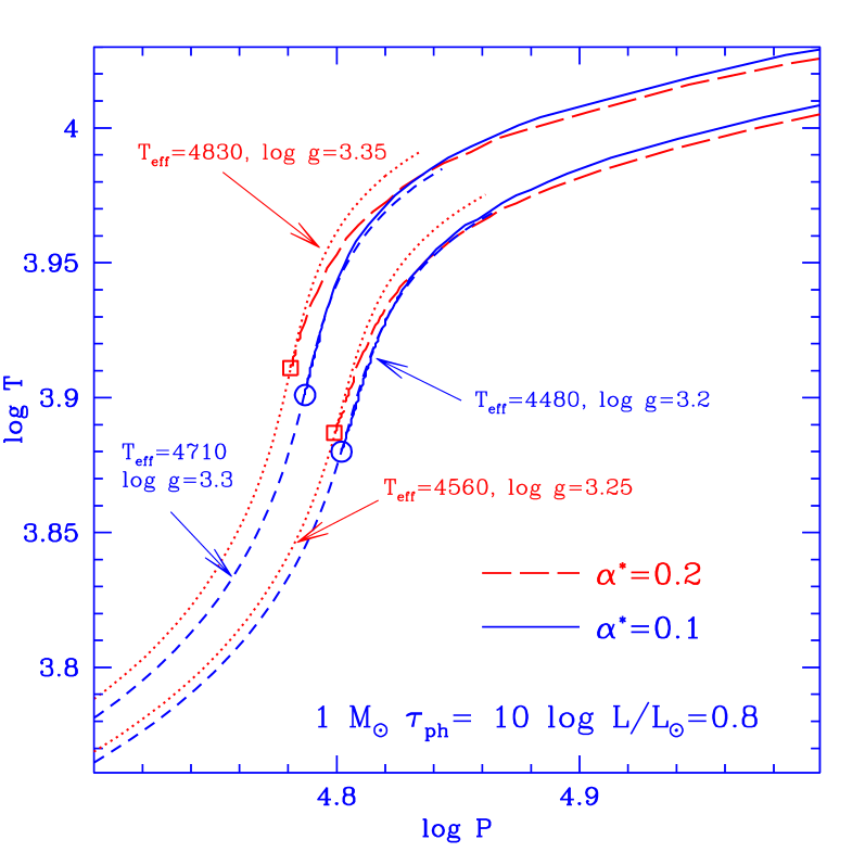
Figure 4: Match between FST internal structure ($\alpha^{*}=0.1$, solid line; $\alpha^{*}$=0.2, long–dashed line) and the corresponding FST atmospheres (short–dashed and dotted lines) for two different evolutionary phases of 1 ${\rm M}_{\odot}$. The models correspond to the square points in Fig. 3

The fine tuning parameter $\alpha^{*}$ for the computation of the interior can also be changed in order to fit the Sun. We will call $\alpha^{*}_{\rm int}$ the parameter used for computation in the interior, in contrast with the fixed value $\alpha^{*}_{\rm atm}=0.09$ adopted in the computation of the grid of atmosphere models.

4 Effect of $\tau_{\rm ph}$ on the evolutionary track location

Since it is not reasonable by now to include a full atmosphere calculation into the computation of a whole stellar model, one separates the internal structure calculation, where the diffusion approximation is used, from the outer part. The calculation of the atmosphere is replaced by the values of the relevant physical quantities at the optical depth $\tau_{\rm ph}$. This $\tau_{\rm ph}$  must be large enough for the diffusion approximation for $\tau>\tau_{\rm{ph}}$ to be valid, and small enough for the approximations adopted for the description of the physics in the atmosphere to hold. Morel et al. (1994) proposed $\tau_{\rm ph}\geq 10$, depending on ${T}_{\rm eff}$ and ${\log g}$ of the model.

If the calculations of the interior and the atmosphere were physically consistent, the stellar models computed with different choices of $\tau_{\rm ph}$ should be equivalent. In practice, the physical inputs such as chemical composition, opacity tables, equation of state, and convection model used in the atmosphere are usually not exactly the same as those used in the interior.

Table 1: Solar–composition computed models

atmosphere		interior		$\tau_{\rm ph}$
ATLAS9 MLT	$\alpha=0.5$	MLT	$\alpha=2.3$	$10^{(3)}$
ATLAS9 MLT	$\alpha=0.5$	MLT	$\alpha=6.3$	$100^{(2)}$
ATLAS9 MLT	$\alpha=0.5$	MLT	$\alpha=1.75$	$1^{(4)}$
ATLAS9 MLT	$\alpha=0.5$	MLT	$\alpha=1.85$	$3$
ATLAS9 FST	$\alpha^{*}=0.1$	FST	$\alpha^{*}=0.1$	1,3,10, 100
ATLAS9 FST	$\alpha^{*}=0.1$	FST	$\alpha^{*}=0.2$	1,3,$10^{(1)}$, 100
AH97 MLT	$\alpha=1.0$	MLT	$\alpha=1.0$	3, 10, 100
AH97 MLT	$\alpha=1.0$	MLT	$\alpha=1.9$	3, 10, $100^{(5)}$

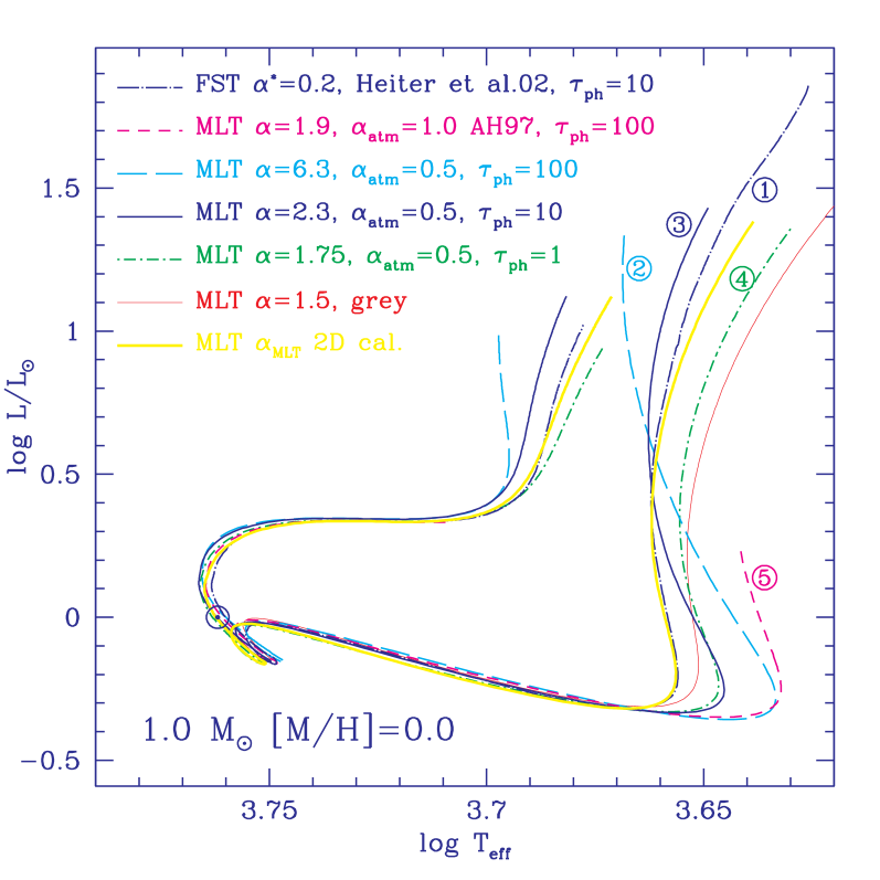
Figure 5: Several evolutionary tracks for 1 ${\rm M}_{\odot}$, solar composition, and MLT treatment of convection in the interior and in the atmosphere. Different values of $\alpha$ for each choice of $\tau_{\rm ph}$ are required to fit the Sun with MLT atmospheres from Heiter et al. (2002a). Besides, a grey MLT model with the same opacity and EOS, and the new FST track with $\alpha^{*}=0.2$ in the interior and FST atmospheres by Heiter et al. (2002a) are plotted. The thick line corresponds to a grey MLT model computed with the $\alpha$ value given by the 2D numerical simulations calibration of Ludwig et al. (1999).

The atmosphere models by Heiter et al. (2002a) adopt the opacity and the equation of state from Kurucz (1993, 1998), while our stellar evolution code considers the micro–physics inputs described in Sect. 3.1. Fig. 3 shows, however, that, if the same convection model (CGM, $\alpha^{*}=0.1$) is used in the atmosphere and in the interior, the HR diagram location of 1 ${\rm M}_{\odot}$ evolutionary tracks is almost independent of the choice of $\tau_{\rm ph}$. Fig. 4 shows the structures ($\log T\,{\rm vs.}\,\log P$) of the interiors and the corresponding atmospheres of 1 ${\rm M}_{\odot}$ models at different evolutionary phases (PMS and Post–MS models marked in Fig. 3 by square points). We see that, in spite of differences in the opacity tables and in the equations of state, the atmosphere structures between $\tau=10$ and 100 almost overlap the values ($\log T\,{\rm vs.}\,\log P$) obtained for the outer layers by integrating the internal structure. The differences introduced in ${T}_{\rm eff}$ due to the different choices $\tau_{\rm ph}$=10 or 100 are smaller than 0.5% along the evolutionary track of 1 ${\rm M}_{\odot}$ with solar metallicity. This is not true if we consider smaller values of $\tau_{\rm ph}$: for $\tau_{\rm ph}$= 1 or $\tau_{\rm ph}$= 3 the differences in temperature gradients between the interior and the atmosphere are larger, because the diffusion approximation of radiative energy transport used in the internal computation is not valid. The temperature gradient computed in the stellar structure code begins to deviate from the atmospheric one at an optical depth lower than $\sim 7$, but the exact point depends on ${T}_{\rm eff}$  and on ${\log g}$. Consequently, the details in the equation of state and opacities are of much less a concern for matching atmosphere and interior models than the region of validity of the diffusion approximation and the modeling of convection, to which we now turn our main attention.

Figure 6: Stellar structure, interior and atmosphere for the solar model corresponding to the labeled evolutionary tracks as obtained with the evolutionary tracks plotted in Fig. 5. MLT models: atmosphere model with $\alpha_{\rm atm}=0.5$, $\tau_{\rm ph}$=100 (long–dashed line), $\tau_{\rm ph}$=10 (solid line), $\tau_{\rm ph}$=1 (short–dashed–dotted line); atmosphere model from AH97, $\alpha_{\rm atm}=1$, $\tau_{\rm ph}$=100 (short–dashed line); FST model (long–dashed–dotted line). The circle, squares, triangle and cross indicate the match point between interior and atmosphere.

4.1 Solar calibrations

It is generally accepted that any stellar modeling must be able to fit the Sun. Two parameters control the Sun’s location in the HR diagram: the helium content which is determined by the solar luminosity, and the jump of specific entropy ($\Delta s$) between the photosphere and the adiabatic convection region (e.g., Christensen-Dalsgaard 1997) which determines the stellar radius.

$$\Delta s=\int_{\ln p_{0}}^{\ln p_{\rm ad}}c_{\rm p}(\nabla-\nabla_{\rm ad})\,d\ln p,$$ (1)

where $p_{0}$ refers to the pressure at a given point in the photosphere, and $p_{\rm ad}$ is the pressure at the point in the convective zone where $(\nabla-\nabla_{\rm ad})\ll 1$.

In MLT, $(\nabla-\nabla_{\rm ad})$ is directly related to the $\alpha$ parameter, and thus varying $\alpha$ allows the fit of solar radius. Hence, depending on the physical inputs, grey models provide values of $\alpha$ between 1.5 and 2.2 (Ventura et al. 1998a). Using the CGM model of convective flux and scale height, only a small variation of $(\nabla-\nabla_{\rm ad})$ can be obtained by varying the tuning parameter $\alpha^{*}$ and for a solar grey model $\alpha^{*}\simeq 0.1$ (CGM, Ventura et al. 1998a) is required. For the present models, using the relations $T(\tau)$ provided by the grids of non–grey atmospheres, the value of $\alpha$ (and $\alpha^{*}$ in the FST, but see later) required to compute the convective envelope fitting the Sun depends also on the choice of $\tau_{\rm ph}$. Eq. (1) can be divided in two terms, $\Delta s_{\rm atm}(\tau_{\rm ph})$ (jump of specific entropy from the surface to $\tau_{\rm ph}$) and $\Delta s_{\rm int}(\tau_{\rm ph})$ ($s$ jump between $\tau_{\rm ph}$ and a layer deep enough where $(\nabla-\nabla_{\rm ad})\sim 0$). Thus, the contribution of the model atmosphere to the entropy jump $\Delta s$ depends crucially on $\tau_{\rm ph}$ and for any chosen $\tau_{\rm ph}$, $\Delta s_{\rm atm}(\tau_{\rm ph})$ must be smaller than $\Delta s$ for a solar model to fit the Sun.

We have considered several combinations of convection treatment in the interior and in the atmosphere, and several choices of $\tau_{\rm ph}$. Table 1 lists the different sets of models computed for the solar composition. The set of parameters fitting the Sun are indicated with a numerical super-script. The value of this index corresponds to the labels in Figs. 5 and 6.

For CGM models, with the non–grey BCs the choice of $\alpha^{*}=0.1$ as derived by the solar calibration with grey BCs provides a Sun $\sim 85$ K cooler than expected. To fit the Sun requires, hence, a larger $\alpha^{*}$ value in the computation of the interior: viz. $\alpha^{*}\sim 0.2$ if $\tau_{\rm ph}$$\leq$10 (Fig. 4). Models computed with consistent $\alpha^{*}$ in the interior and in the atmosphere would have an intermediate value of $\alpha^{*}$. As shown in Fig. 4, an increase of $\alpha^{*}$ by a factor 2 implies a lower temperature gradient in the layers deeper than $\tau_{\rm ph}$=10 and hence a higher ${T}_{\rm eff}$. The term $\alpha^{*}H_{\rm p}(\tau_{0})$, however, affects only the scale length close to the boundary of the convective zone. Since the efficiency of FST convection rapidly increases downwards the convective zone, the atmosphere at $\tau=100$ is quasi-adiabatic (see Fig. 2) and hence even a value of $\alpha^{*}$ larger, but restricted to the interior, cannot increase the entropy in the adiabatic region. This explains what is meant by saying that the FST model with the scale length as in Eq. (3.3)–(3.3), or equivalently with the original suggestion from Canuto et al. (1996), is less parametric than standard MLT: if an FST–based solar model fails to fit the Sun, there is less possibility of achieving anyway a match by adjusting $\alpha^{*}$, as this parameter only provides some fine tuning.

Concerning the MLT calibration, Fig. 2 shows an atmosphere with ${T}_{\rm eff}$ and ${\log g}$ close to the solar values. The over-adiabaticity is quite high up to $\tau=100$ and therefore $\Delta s_{\rm atm}(\mbox{$\tau_{\rm ph}$}=100)\gg\Delta s_{\rm atm}(\mbox{$\tau_{\rm ph}$}=10)$. To keep $\Delta s$ in the range required to fit the solar radius, the contribution of the term $\Delta s_{\rm int}(\tau_{\rm ph})$ is controlled by increasing $\alpha_{\rm int}$ since $(\nabla-\nabla_{\rm ad})\sim\alpha^{-4/3}$ in the high efficiency limit. This explains the very different values of $\alpha_{\rm int}$ required with different $\tau_{\rm ph}$’s ($\alpha_{\rm int}=2.3$ for $\tau_{\rm ph}$=10, and $\alpha_{\rm int}=6.3$ for $\tau_{\rm ph}$=100). Obviously, this results in a kink at the connection point, inducing discontinuities in the derivatives of the temperature gradient and in the over–adiabaticity (cf. Fig. 6). A temperature structure similar to that obtained with FST could be obtained with MLT and a variable length scale, as in Schlattl et al. (1997). These authors found that between $\tau(T=T_{\rm eff})$ and $\tau=20$ a MLT 1-D atmosphere, computed with $\alpha=0.5$, agrees very well with the 2D–hydrodynamical model from Freytag et al. (1996). Hence they decided to use a model atmosphere computed with $\alpha=0.5$ down to $\tau=20$ and introduced a mixing-length parameter $\alpha=\alpha(\tau)$ whose dependence on $\tau$ was chosen to model the temperature–pressure stratification of the 2D–model, and the parameters to fit the solar values of ${T}_{\rm eff}$ and luminosity (see their Fig. 1).

Clearly, such procedures can be applied to the solar case, but how to extrapolate them to other regions of the HR diagram? Although these MLT-based models are built in such a way that the atmospheric convection prescription fits the solar Balmer lines better than the standard models with large $\alpha$, and the internal structure integration fits the present solar radius, we have to warn about the poor physical meaning of extending this procedure to structures different from the Sun. To fit the Sun, the low $\alpha=0.5$ needed in the atmosphere is compensated by the larger value adopted in the interior, but the effect on the evolutionary track of a different $\alpha$-value below $\tau_{\rm ph}$, is not the same over the whole HR diagram. As shown in Fig. 5, very different PMS evolutionary tracks (by ${T}_{\rm eff}$ and shape) are obtained with parameter sets all fitting the HRD location of the Sun. We note that the PMS track of the 1 ${\rm M}_{\odot}$ model, obtained integrating the interior up to $\tau_{\rm ph}$=1, is, as expected, quite close to the MLT grey model. Moreover the coolest low–PMS tracks are obtained when the integration of the atmosphere (with low efficiency convection, $\alpha_{\rm atm}=0.5$, or 1.0) goes down to $\tau_{\rm ph}$=100. But, which are the good PMS tracks: those obtained with $\tau_{\rm ph}$=10, or with $\tau_{\rm ph}$=100? The convection properties of stellar layers at $\tau_{\rm ph}$ are not the same all over the HR diagram. The fraction of the over-adiabatic region above $\tau_{\rm ph}$  depends on ${T}_{\rm eff}$ and ${\log g}$. So, there is no physical reason in choosing an efficiency of convection below $\tau_{\rm ph}$ and another above that point. The only justification for doing so could be the match of a larger set of observed data, but this procedure would require calibration standards throughout the HR diagram. On the other hand, the procedure of mixing very different treatments of convection, based on solar calibration, finally results in physical inconsistencies, introduces a large dispersion ($\sim 200$ K) in the low gravity region of the HR diagram (see Fig. 5), and reduces even more the predictive power of MLT based stellar modeling.

Ludwig et al. (1999) proposed a calibration of the $\alpha(\mbox{${T}_{\rm eff}$},\mbox{${\log g}$})$ providing the same specific entropy jump in a grey atmosphere as their 2-D numerical simulations, and therefore, the same stellar radius (although this does not imply the model will also have a realistic sub-photospheric stellar structure). The thick line in Fig. 5 was computed with the same EOS and opacity tables, but adopting a grey atmosphere and MLT with the $\alpha(\mbox{${T}_{\rm eff}$},\mbox{${\log g}$})$ 2D-based calibration. We see that for $\log L/L_{\odot}<0.75$ this track almost overlaps that obtained by non-grey FST modeling.

Fig. 6 shows how different the sub–atmospheric layers of the “Sun’s” can be, as obtained from five sets of parameters fitting the solar ${T}_{\rm eff}$ and radius. Thanks to helioseismology it is possible to get information about the interior of the Sun, and several authors (Baturin & Miranova, 1995; Monteiro et al. 1995; and Heiter et al. 2002b from non–grey MLT and FST models) have concluded that FST solar models yield sound velocities as a function of depth, which are in better agreement with the helioseismological data. Schlattl et al. (1997) as well, with their spatially varying mixing length parameter, obtained clear improvements with respect to previous computations. It has to be noticed that even if the abrupt change of slope in the temperature profiles #2 and #3 of Fig. 6 is adequately smoothed, the frequencies resulting from both kinds of sub-atmospheric structures (FST and MLT with $\tau_{\rm ph}$=10) will be different and their differences can hence be probed by helioseismology.

The matching of model atmospheres on top of interior structure calculations raises the question if it is possible to put a constraint on the optical depth where convection becomes efficient and if low values of $\alpha$ in an MLT treatment can be excluded. The case of stars with shallow — in terms of $H_{\rm p}$ — surface convection zones, such as A–type main sequence stars, can be described in terms of inefficient convection throughout the convective zone, from an observational point of view (Smalley & Kupka 1997, Heiter et al. 2002a, Smalley et al. 2002), from the results of non–local convection models without a mixing length, and from numerical simulations (see the discussion in Kupka & Montgomery 2002, and Freytag 1995). Unfortunately, for stars with deep envelope convective zones the interpretation of the observational data remains ambiguous (cf. also Castelli et al. 1997, Heiter et al. 2002a) and the comparison with numerical simulations provides no simple alternative, i.e. a parameterization of temperature and pressure as a function of depth which could simultaneously fit both the stellar radii and the spectroscopic and photometric data. Obviously, the calibration problem becomes even worse for the case of evolutionary tracks running through extended regions of the HR diagram. In comparison with MLT, the FST based models offer the advantage of agreeing with more observational data without the need of drastically changing the scale length at some ill–defined matching depth, which, in the end, introduces at least another free parameter. Nevertheless, the discrepancies of these models with observed color photometry for the Sun (Smalley & Kupka 1997 and references therein) and with temperature gradients as obtained from various 3D large eddy simulations of solar granulation call for urgent further improvement in convection modeling.

5 Convection treatment and PMS location

From Fig. 5 it is clear that HR diagram location of the Hayashi tracks is strongly model-dependent, and the models with different convection treatment —even selecting only those models fitting the Sun— provide tracks of very different shapes and ${T}_{\rm eff}$  ranges (see also the first discussion given by D’Antona and Mazzitelli 1994). In this section we show the origin of differences and similarities among available PMS evolutionary tracks, often used in comparing and interpreting observational data.

5.1 FST based models

In this section we analyze the effect of different formulations of the FST model (different $\alpha^{*}$, plus the grey model) on the PMS evolution. As seen in the previous section, the solar calibration with non–grey BCs requires a tuning of the parameter $\alpha^{*}$  larger by a factor of two with respect to that used for the atmospheric grids. No feature from spectra and colors can constrain this parameter, but the deep structure of the atmosphere will be slightly different. The new value $\alpha^{*}=0.2$ required when $\tau_{\rm ph}$$\leq$10 is anyway within the limits given for stellar “overshooting” (Maeder & Meynet 1991). In principle, an inconsistency is introduced in this way between the treatment of convection in outer and internal layers. The effects of this inconsistency on the HR diagram are small, but different for each (${T}_{\rm eff}$, ${\log g}$). For ${T}_{\rm eff}$$<4700K$ the atmospheric convection begins at increasingly shallower layers and becomes almost adiabatic deep in the FST atmosphere (see curve corresponding to ${T}_{\rm eff}$=4400 K and ${\log g}$=3.8 in Fig. 2). This explains the small effect of different $\alpha^{*}$ on the PMS tracks location in right side of the HRD compared with the effect on the PMS tracks corresponding to the highest masses considered.

Fig. 7 shows the evolutionary tracks for masses from 0.6 to 2.0 ${\rm M}_{\odot}$ obtained using: i) exactly the same treatment of convection in the atmosphere and inside the star (dotted lines), i.e.  CGM fluxes and scale length with $\alpha^{*}=0.1$; and ii) a slightly different scale length with $\alpha_{\rm atm}^{*}=0.1$, and $\alpha^{*}=0.2$ below $\tau_{\rm ph}$=10. The effect on ${T}_{\rm eff}$ of changing $\alpha^{*}$ by a factor 2 will depend on the quantity $a=(\Lambda_{\rm atm}+\Lambda_{\rm int})/(\alpha^{*}H_{\rm p})$ (where $\Lambda_{\rm atm}$ is the extent of the convection zone for $\tau<\tau_{\rm ph}$ and $\Lambda_{\rm int}$ is the distance to $\tau_{\rm ph}$). If $a$ is much larger than one, the variation of ${T}_{\rm eff}$ will be negligible as the convective flux and the temperature gradients will not change. On the contrary, if it is of the order of one or smaller, the effect on the temperature gradients for the last points of the structure will be significant and as the gradients decrease, the ${T}_{\rm eff}$’s increase. The differences of ${T}_{\rm eff}$, at constant luminosity, induced by the tuning of $\alpha^{*}$ go from $\sim 30$ K at the lowest masses, to $\sim 80$ K for 1.5 ${\rm M}_{\odot}$, and $\sim 120$ K for 2.0 ${\rm M}_{\odot}$. This implies that, at given $L$ and $M$, the maximum uncertainty introduced in ${T}_{\rm eff}$ is $\sim 2$% ($<\,1$% for 1 ${\rm M}_{\odot}$); and, at a given $L$ and ${T}_{\rm eff}$ the maximum uncertainty in mass is $\sim 17$%.

Fig. 8 shows the effect of non–grey BCs on the location of the Hayashi tracks. DM97, 98 models were computed with the CGM formulation of convection in the interior and with grey BCs. The authors approached the problem of convection penetrating in the atmospheres of low–gravity/low–temperature models, integrating the interior until the top of the convective region. The present “complete” (and more physically coherent) FST models are much cooler than the grey ones, $\sim 270$ K for the lowest computed masses.

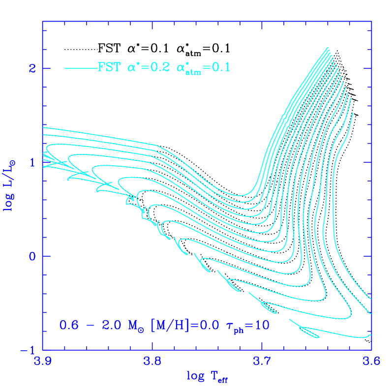
Figure 7: FST evolutionary tracks with ATLAS9-FST atmospheres with $\alpha^{*}=0.1$

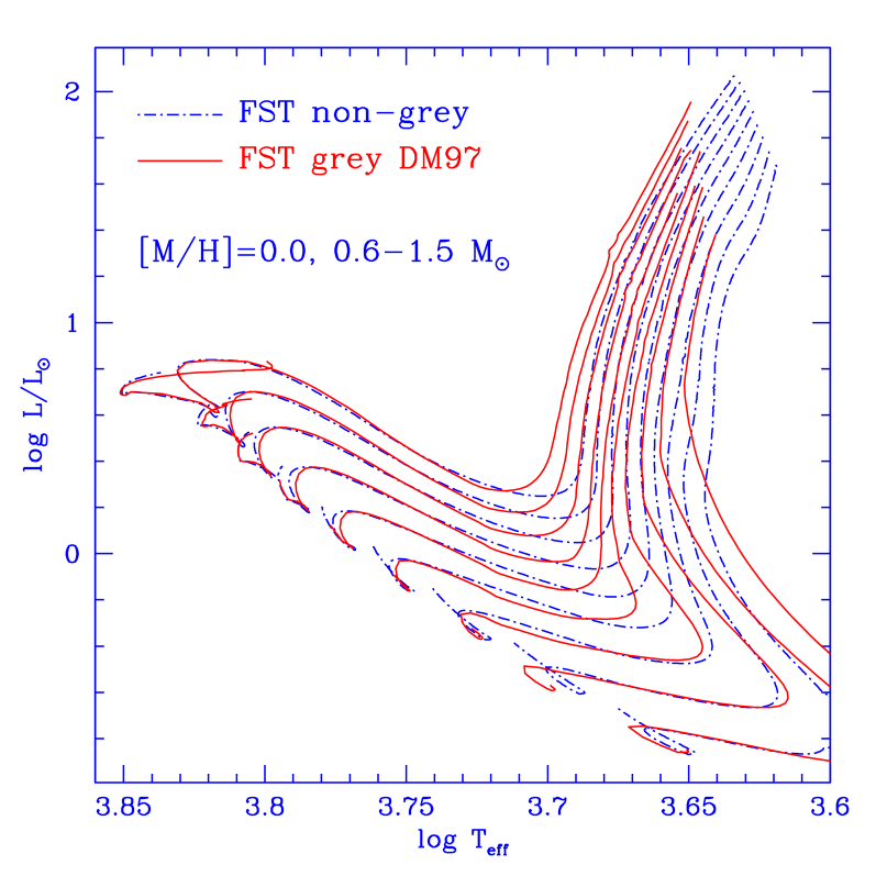
Figure 8: Comparison between FST grey models (DM97), and ”complete” FST models with the new ATLAS9 atmosphere models

5.2 Effect of different MLT prescriptions

We computed as well two grids of stellar models with the same micro–physics in the interior, but using NextGen atmosphere models (AH97) as BCs. NextGen includes a large number of molecular lines which, being the main source of opacity for low–temperature models, must have a significant role in the onset of convection. These models use MLT with $\alpha=1.0$ and provide super-adiabatic gradients smaller than those from the new ATLAS9 models. As a consequence, adiabaticity is reached at lower depths than in ATLAS9 (MLT $\alpha=0.5$) models and there is a smaller difference in choosing either $\tau_{\rm ph}$=10 or $\tau_{\rm ph}$=100.

Anyway, the value $\alpha_{\rm int}=1$ is too small to fit the solar radius, for which $\alpha_{\rm int}=1.9$ is required. Fig. 9 shows the tracks computed with NextGen atmospheres ($\alpha_{\rm atm}=1.0$) down to $\tau_{\rm ph}$=100, and with $\alpha_{\rm int}=1.0$ (dash-dotted curve) and $\alpha_{\rm int}=1.9$ (solid line) for all layers below. These curves are equivalent to those published by Baraffe et al. (1998, BCAH98). We point out that there is a large difference in ${T}_{\rm eff}$  ($\sim$380 K in MS and 440 K in PMS for a  1${\rm M}_{\odot}$  model) and that the shape of the Hayashi tracks as well changes with the $\alpha$–value adopted in the interior. The NextGen tracks with the parameter fitting the Sun ($\alpha_{\rm atm}=1.0$ down to $\tau_{\rm ph}$=100 and $\alpha_{\rm int}=1.9$) are cooler than ATLAS9 tracks with $\alpha_{\rm atm}=0.5$ down to $\tau_{\rm ph}$=10 and $\alpha_{\rm int}=2.3$. But Fig. 5 shows that ${T}_{\rm eff}$ values as low as in NextGen models can be obtained using the ATLAS9-tracks with $\alpha_{\rm atm}=0.5$, $\tau_{\rm ph}$=100 and $\alpha_{\rm int}=6.3$. The reason is just that, when we integrate the atmosphere down to $\tau_{\rm ph}$=100, we adopt a lower efficiency of convection in a larger region, and so the ${T}_{\rm eff}$ of the model decreases.

Figure 9: MLT PMS tracks obtained using as BCs the atmosphere models by AH97 ($\alpha=1$), with two different values of $\alpha$ in the computation of the sub-atmospheric convection and with the match point as in BCAH98, $\tau_{\rm ph}$=100.

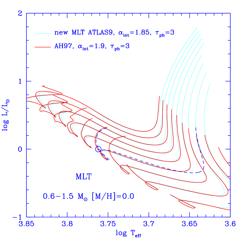
Figure 10: Comparison between MLT models using ATLAS9 atmospheres and AH97 atmospheres until $\tau_{\rm ph}$=3. In both cases the parameters are chosen to fit the Sun. The dashed-line is a 1 ${\rm M}_{\odot}$ evolutionary track computed with $\alpha_{\rm int}=1.9$ and with AH97 atmospheres until $\tau_{\rm ph}$=100.

We computed stellar models for AH97 BCs with $\alpha_{\rm int}=1$ and $\alpha_{\rm int}=1.9$, for three different choices of $\tau_{\rm ph}$ (3, 10 and 100). As in the FST case (Sect. 4), when we use $\alpha_{\rm int}=1.0$, the same as in the atmosphere models, there is only a small difference between evolutionary tracks whose interior has been integrated until $\tau_{\rm ph}$=3, 10, or 100. The difference between $\tau_{\rm ph}$=3 and $\tau_{\rm ph}$=100 tracks, due to the incoherence introduced by the diffusion approximation used in the interior integration, is of the order of 40 K in the low-gravity domain. When we use $\alpha_{\rm int}=1.9$, but the atmospheric grids still have $\alpha=1.0$, the PMS track location depends as well on $\tau_{\rm ph}$. Thus, the $\tau_{\rm ph}$=3 tracks are now $\sim 170$ K hotter than the $\tau_{\rm ph}$=100 tracks (see Fig. 10 for the relative location of 1${\rm M}_{\odot}$  tracks, thick-solid line and dashed line).

In Fig. 10 we plot the evolutionary tracks calibrated on the Sun and integrating the internal structure up to $\tau_{\rm ph}$=3 for both atmosphere models, NextGen and new MLT ATLAS9 models. The overlap of both sets of models for the whole common ${T}_{\rm eff}$/${\log g}$  domain is, at first sight, surprising: it points out the similarity of the opacity in the atmosphere models (NextGen versus ATLAS9) in this domain. Generally, at $\tau=3$ the gradient of temperature still follows the radiative gradient of temperature, and hence the convective fluxes and the choice of $\alpha_{\rm atm}$ do not have a relevant role.

These results confirm that for ${T}_{\rm eff}$$\geq$4000 K the convection model is much more important than the contribution of additional molecules to opacity already included in ATLAS9 (as concluded by DM94 on the basis of grey models).

5.3 FST versus MLT

The main difference between FST and MLT that we must keep in mind is that in the region of low efficiency FST is much less efficient, while, in the high efficiency region, the FST convective fluxes are $\sim$10 larger than the MLT ones, so FST describes a much more efficient convection in deep layers. This means that, deep in the atmosphere, the MLT models yield higher temperature gradients than the FST ones (cf. Fig. 6 for $\log(P)>5.3$), and hence lower ${T}_{\rm eff}$. DM97, 98 showed that, when grey BCs are used, the difference in ${T}_{\rm eff}$ between FST and MLT tracks for solar mass tracks fitting the Sun was in between 5–10% ($\sim 250$ K for 1 ${\rm M}_{\odot}$). This difference is relatively small in absolute value, but quite large, if we consider that PMS tracks of different masses are nearly parallel and rather close to each other. Thus, the masses of TTauri determined by comparison between their location on the HRD and either the MLT or FST evolutionary tracks, could differ up to 50%.

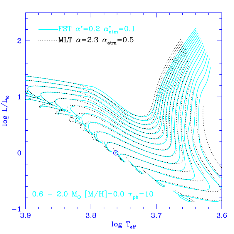
Figure 11: PMS tracks obtained using parameters that fit the Sun, for FST and MLT treatment of convection using the new MLT and FST ATLAS9 atmosphere models

If non–grey BCs are used, the ${T}_{\rm eff}$ location of MLT tracks also depends on $\tau_{\rm ph}$  and therefore a direct comparison with FST tracks is not obvious. Fig. 11 shows the new FST and MLT Hayashi tracks computed with the parameters ($\alpha^{*}$ and $\alpha$) calibrated on the Sun and $\tau_{\rm ph}$=10. We note that the differences increase as the stellar mass decreases, and they are almost negligible for $M\geq 1$ ${\rm M}_{\odot}$. There are two reasons that explain why the MLT and FST tracks are now so close to each other: i) Fig. 1 shows that there is a domain in (${T}_{\rm eff}$, ${\log g}$) where both sets of atmosphere models with low convection efficiency provide very similar atmospheric structures for $\tau\leq 10$, and hence similar BCs. ii) The low efficiency of MLT convection below $\tau=10$ is more or less compensated by a higher value of $\alpha$ (2.3) in the interior. The total effect is such that the largest differences in ${T}_{\rm eff}$ are of the order of 100 K ($\sim 2$%), that induce an uncertainty in the mass determination of observed PMS stars between 10–17%.

Note also the difference between FST and MLT MS models at $\sim 6500$ K, where convection in the atmosphere is highly inefficient (this can be expected from their different atmospheric temperature structure as shown by Fig. 1, see also D’Antona et al. 2002).

6 Metallicity and PMS location

We have computed FST-based models also for two other metallicities, [M/H]=–0.3 and +0.3. All of them included the CGM convection model with $\alpha^{*}=0.1$ until $\tau_{\rm ph}$=10, and $\alpha^{*}=0.2$ for the layers below. Fig. 12 shows that changes of the chemical composition by a factor 2 with respect to the solar one produce a small effect on the ${T}_{\rm eff}$ location of PMS tracks for FST models: $\sim 100$ K hotter for [M/H]=–0.3 and $\sim 100$ K cooler for [M/H]=+0.3. In Fig. 13 we compare our FST models with MLT models by Siess et al. (2000) for 1 ${\rm M}_{\odot}$. At $\log L/L_{\odot}=0.6$, the FST–based model with [M/H]=–0.3 is $\sim 130$ K hotter than that one with solar composition, while MLT models differ by $\sim 170$ K. Note that in the Siess et al. (2000) models the Z=0.02 solar track does not fit the solar ${T}_{\rm eff}$. Nevertheless, the Siess et al. solar metallicity (Z=0.02) PMS models, being cooler, do not make a bad job in reproducing the observations, according to the analysis by Simon et al. (2000).

Figure 12: PMS tracks of 2.0, 1.0, and 0.6 ${\rm M}_{\odot}$ stars for three different chemical compositions ($[M/H]=-0.3,0.0,+0.3$). All these tracks have been computed using as boundary conditions the new ATLAS9 (CGM, $\alpha^{*}=0.1$) atmosphere models at $\tau_{\rm ph}$=10 and the CGM formalism for the convection in the interior with $\alpha^{*}=0.2$.

Figure 13: Evolutionary tracks for 1 ${\rm M}_{\odot}$ for metallicity $Z=0.01$ and $Z=0.02$ ($Z_{\odot}$) and two treatments of convection: FST with $\alpha^{*}=0.2$ and MLT from Siess et al. (2000).

Figure 14: The mass determined from the HR diagram position with respect to the evolutionary FST tracks is plotted with respect to the dynamical mass for the double lined spectroscopic and eclipsing binary RXJ0529.4+0041 (full circles); the other points are for the double lined spectroscopic binaries RXJ0541.4-0324 (empty squares); RXJ0532.1-0732 (empty triangles); RXJ0530.7-0.434 (empty circle, only one because $M$,${T}_{\rm eff}$ and $L$ are the same for both stars), in which the minimum dynamical mass is plotted. The data are from Covino et al. 2001. In addition, the location of TYCrA (full triangle) (Casey et al. 1998) and GMAur (full square) (Dutrey et al. 1998) is shown.

7 Comparison with the observations

The theoretical uncertainties in the location of the PMS, confirmed in the present computation, are such that direct mass determinations of PMS are needed to constrain the models. In particular, the eclipsing double–lined spectroscopic binaries allow simultaneous determination of masses and radii of the components. Only one binary of this type is known by now to contain two PMS components, namely RXJ 0529.4+0041 (Covino et al. 2000) while several other PMS spectroscopic double–lined non–eclipsing binaries (Melo et al. 2001) can just constrain the minimum mass of the components. In Fig. 14 we plot the masses derived by comparing the observationally derived ${T}_{\rm eff}$ (and luminosity) with the theoretical evolutionary FST-tracks versus the dynamical masses. The error bar on the theoretical mass reflects the observational error on the temperatures quoted by the authors ($\sim 100-200$ K). A very small error is generally attributed to the dynamical masses. Apart from the case of RXJ 0529.4+0041, for which the inclination $i$ is known, the plotted dynamical mass is the minimum mass $Msin^{3}i$. Many points remain below the diagonal line in Fig. 14, and the discrepancy could be larger if we had a precise indication of an $i<90$. This result, although still preliminary in view of the very few observational points and of the uncertainty of ${T}_{\rm eff}$  determination of the PMS objects, indicates that even with the inclusion of non–grey FST model atmospheres, the FST convection is too efficient to describe the PMS. Moreover it confirms the preliminary comparisons based on grey FST models by Simon et al. (2000) and Covino et al. (2001). It is possible that the error bars on ${T}_{\rm eff}$ as provided by the authors were underestimated. In order to make the mass derived for the coolest component of RXJ 0529.4+0041 compatible with observations, the error bar should grow up to $\sim 400$ K. Since the PMS-FST tracks are very close to each other in ${T}_{\rm eff}$ (at $\log L/L_{\odot}=0.3$,  $\Delta$${T}_{\rm eff}$ between 1.5 and 0.6 ${\rm M}_{\odot}$ is only $\sim$650K), such a large error in ${T}_{\rm eff}$ also for the other stars would imply, however, that no useful constraint on the models could be obtained from this comparison.

Baraffe et al. (2002) found that most masses in PMS binaries are better reproduced with $\alpha_{\rm int}=1.9$, but some others require $\alpha_{\rm int}=1$, while in principle there is no physical reason to justify this difference in the efficiency of convection in the same region of the HR diagram. In fact, we have seen in Sect. 5 (Fig. 9) that for a given mass, the MLT tracks may differ even by 500 K if we consider both models with small and large $\alpha$ and disregard any solar constraint. Furthermore, for solar calibrated models, a variation of $\tau_{\rm ph}$ from 3 to 100 could produce a displacement of their PMS tracks of the order of 200 K (compare Fig. 9 with Fig. 10). No progress in understanding is possible with this philosophy. In particular, there may be hidden parameters which affect the tracks location that could not be isolated unless we can — at least in part — falsify the models.

FST, contrarily, does not allow large displacements on the HRD by changing the parameters. The FST convection has also been shown to be very useful both to describe the solar structure (see the introduction) and many other different evolutionary phases (e.g. the DB white dwarfs pulsation boundary –Benvenuto & Althaus 1997–, the Hot Bottom Burning phase in the intermediate mass Asymptotic Giant Branch stars –Ventura et al. 2001 and 2002–, the fast transition between deep and atmospheric convection in main sequence stars –D’Antona et al. 2002): this may lead us to suspect that there is some other physical input specific of PMS models, which modifies convection in the PMS stars. Just as an example, we notice that GM Aur, which has a dynamical mass estimation of $0.84\pm 0.05$ ${\rm M}_{\odot}$ (Dutrey et al. 1998) and an evolutionary mass of $0.5\pm 0.2$ ${\rm M}_{\odot}$ also shows a magnetic field of $4-5\,10^{3}$  Gauss (Johns-Krull et al. 1999). D’Antona et al. (2000) have shown that the purely thermal effect of a magnetic field deeply modifies the behavior of atmospheric convection, precisely in the required direction of enlarging the temperature gradients and lowering the models ${T}_{\rm eff}$.

8 Summary and Conclusions

The new ATLAS9 atmosphere models based on the CGM treatment of convection have allowed us to compute, for $\mbox{${T}_{\rm eff}$}\ >4000$ K and three different metallicities, new grids of non-grey FST-PMS evolutionary tracks with the same convection treatment in the interior and in the atmosphere. They provide a significant improvement with respect to DM97,98 grey FST-PMS tracks. Furthermore, we have examined one by one the parameters affecting the $T_{\rm eff}$ location of PMS tracks analyzing the “traps” hidden in the modeling of convection in PMS and taking advantage of the use of new grids of stellar atmospheres constructed with different assumptions for convection.

Concerning the choice of the match point $\tau_{\rm ph}$ between the atmosphere and the interior, we have pointed out that the differences between the micro–physics (opacity tables and equation of state) inputs in the interior and the atmosphere models introduce a negligible uncertainty on the derived HRD location. Actually, the spatial resolution of the deepest layers of the atmosphere model is much more relevant for the choice of $\tau_{\rm ph}$. We have seen that low resolution models could induce non–negligible errors in the BCs, especially if $\tau_{\rm ph}$=100 is taken as the match point between atmosphere and interior. This choice may otherwise appear more suitable due to the flatter temperature gradient and the ascertained validity of the diffusion approximation of radiative transfer at this depth.

We show that, while a successful solar calibration of a 1${\rm M}_{\odot}$ model adopting a low efficiency of convection in the atmosphere can be achieved by adequately increasing the efficiency of convection in the interior, sets of parameters which allow obtaining a good solar radius do not provide the same PMS tracks. In fact, different couples of parameters ($\alpha_{\rm int}$,$\tau_{\rm ph}$) introduce a dispersion in the ${T}_{\rm eff}$ of the PMS track of 1${\rm M}_{\odot}$ of the order of 200 K (if we take into account also the FST track, the uncertainty on ${T}_{\rm eff}$ grow up to 250 K). Since there is no physical reason to have a different efficiency of convection at each side of a fixed $\tau_{\rm ph}$, the introduction of another parameter reduces significantly the predictive power of such models: in non–grey stellar models computed using different convection in the interior and in the atmosphere, the parameters are at least three: $\alpha_{\rm int}$, $\alpha_{\rm atm}$ and $\tau_{\rm ph}$.

While in the MLT models the value $\alpha_{\rm atm}=0.5$ is chosen to fit the Balmer lines, in the CGM ones, the fine tuning parameter $\alpha^{*}$ cannot be constrained by the spectral features of solar type stars, since $\alpha^{*}$ affects mainly the gradients in the deep layers of the solar atmosphere. The value adopted from the grey solar calibration by Canuto et al. (1996) turns out to be too low for the non-grey model of the Sun, and a variation of $\alpha^{*}_{\rm int}$ of a factor of two with respect to $\alpha_{\rm atm}^{*}$ is required. A solar model with exactly the same convection treatment in the interior and in the atmosphere should adopt an intermediate value of $\alpha^{*}$. Nevertheless, by changing $\alpha_{\rm int}^{*}$ within this range we are not able to produce significant displacements over the HR diagram, and the $\Delta\mbox{${T}_{\rm eff}$}$ on the PMS tracks due to this change is smaller than 100 K for $M<$ 1.5${\rm M}_{\odot}$.

The evolutionary track using grey atmospheres and a MLT treatment of convection with a $\alpha(\mbox{${T}_{\rm eff}$},\mbox{${\log g}$})$ value provided by the 2D-model calibration (Ludwig et al. 1999) is quite close (in a large ${\log g}$ /${T}_{\rm eff}$ domain) to that one obtained with a non-grey FST model fitting the Sun. This implies that the specific entropy jump between the photosphere and the adiabatic zone is almost the same in the FST based models and in the 2D-hydrodynamical atmosphere models. However, one should expect the specific entropy jump and hence PMS evolutionary tracks obtained from a 3D-hydrodynamical model atmosphere calibration to be different. As shown by Asplund et al. (2000), for solar surface convection numerical simulations in 2D yield higher temperatures in the deeper layers and lower ones in optically thin regions when compared to their 3D counterparts (see their Fig. 9). The calibration by Trampedach et al. (1999) which is based on such 3D numerical simulations cannot be used safely to calculate PMS evolutionary tracks, because the model calculations used to derive the coefficients of their fitting functions are limited to essentially the main sequence band. Ludwig et al. (1999) explicitly warn their readers that their fits quickly loose their meaning outside the region covered by their own model grid. Fortunately, their grids have been computed for a much wider region of the HRD which in fact is just large enough to include the solar PMS track as shown in Fig. 5 within the domain valid for their calibration.

We obtain quite similar PMS tracks in some regions of the HRD by using FST or MLT ($\alpha_{\rm atm}=0.5$, $\alpha_{\rm int}=2.3$, $\tau_{\rm ph}$=10) stellar models. The reason is that MLT ($\alpha=0.5$) and FST atmospheres have ($P,T$) structures which overlap for optical depths smaller than $\tau\sim 10$, and the higher efficiency of FST at larger optical depths is compensated by a larger value of the mixing length parameter. The maximum $\Delta\mbox{${T}_{\rm eff}$}$ is of the order of 100 K, for the lowest considered masses.

The comparison between AH97 and the new ATLAS9-based models shows that: i) both sets of models are equivalent if the match point between atmosphere and internal structure is chosen not too deep in the atmosphere (e.g. $\tau_{\rm ph}$=3, Fig. 10). Since in this region the temperature gradient follows the radiative gradient, and the radiative gradient is determined mainly by the opacity, the overlapping between both sets of models all over the ${T}_{\rm eff}$-${\log g}$ domain considered allows us to conclude that the improvement of opacity in AH97 models has no relevant role for the location of stellar evolution tracks in this region of the HR diagram; ii) the differences between MLT-ATLAS9 models and AH97 models are only due to the specific treatment of the over–adiabatic convection. Therefore, at ${T}_{\rm eff}$$\geq$4000 K the convection model is much more important than the contribution of additional molecules to the opacity already included in ATLAS9 (as concluded by DM94 on the basis of grey models).

Examining some PMS binaries,which provide independent determination of the stellar masses, the new FST $\tau_{\rm ph}$=10 models provide an on average too efficient convection with respect to the masses and HR diagram location of these binaries. Covino et al. (2001) and Steffen et al. (2001) found that the best fit is obtained when MLT with $\alpha=1$ (in the interior and in the atmosphere) is adopted. Since MLT based models must adopt a value of $\alpha$ larger than 1 to fit the Sun, and since FST treatment (that provides a quite efficient convection) is able to fit the solar radius, the comparison with observation suggests that convection in the PMS evolutionary phase seems to be less efficient than for the Sun. The FST model cannot be tuned too much, but it nevertheless provides very valuable results for many different evolutionary phases. Therefore, instead of dismissing the model at this point, we suggest that there may still be another physical parameter affecting the location of PMS tracks in the HR diagram. Processes such as, e.g., interaction with a circumstellar disk (Flaccomio et al. 2003), acceleration and/or braking of rotational velocity during PMS evolutionary phase, or presence of a dynamo magnetic field (Ventura et al. 1998b, D’Antona et al. 2000) could modify the convective temperature gradients in the outer layers of PMS stars.

Finally, also the sub-photospheric structures of the Sun, as obtained by different choices of BCs and convection modeling, are quite different. The helioseismological data allow now to discriminate between different solar structures and indicate that the Sun is better reproduced with the FST-based model than with the MLT one. However, there are other aspects of surface convection in the Sun that cannot be fitted with a local 1D model such as FST, as discussed in Sect. 3.2.1 and 4.1 and in references cited therein. Major progress towards non-local and non-homogeneous models of convection suitable for evolutionary track computations is thus urgently needed to improve current stellar models.

- (1) Alexander D.R., Ferguson J.W., 1994, ApJ 437, 879
- (2) Allard F., Hauschildt P., 1997 (AH97) NextGen
- (3) Asplund M., Ludwig H.-G., Nordlund Å., & Stein R.F., 2000, 359, 669
- (4) Baraffe I., Chabrier G., 1997, A&A 327, 1039
- Baraffe, Chabrier, Allard, & Hauschildt (1995) Baraffe I., Chabrier G., Allard F., & Hauschildt P. H., 1995, ApJL, 446, L35
- (6) Baraffe I., Chabrier G., Allard F., Hauschildt P., 1998, A&A 337, 403 (BCAH98)
- (7) Baraffe I., Chabrier G., Allard F., Hauschildt P., 2002, A&A 382, 563
- (8) Baturin V.A., Mironova I.V., 1995, AZh 72, 120 L65
- Benvenuto & Althaus (1997) Benvenuto, O. G. & Althaus, L. G. 1997, MNRAS, 288, 1004
- (10) Bernkopf J., 1998, A&A 332, 127
- (11) Böhm K.H., Stückl, E.,1967 Zeitschrift f r Astrophysik 66, 487
- (12) Böhm-Vitense E., 1958, Z. Astrophys. 46, 108
- (13) Canuto V.M., 1992, ApJ 392, 218
- (14) Canuto V.M., 1996, ApJ 467, 385
- (15) Canuto V.M., Mazzitelli I., 1991, ApJ 370, 295
- (16) Canuto V.M., Goldman I., Mazzitelli I., 1996, ApJ 473, 550
- (17) Casey B.W., Mathieu R.D., Vaz L.P.R., Anderson J., Suntzeff N.B. 1998, AJ 115, 1617
- (18) Castaing B., Gunaratne F., Helsot F., Kadanoff L., Libchaber A., Thomae S., Wu X.Z., Zaleski S., Zanetti G., 1989, J. Fluid Mech. 204, 1
- (19) Castelli F., 1996, in Adelman S.J., Kupka F., Weiss, W.W., Model Atmospheres and Spectrum Synthesis, 1996, ASP Conf. Ser. Vol. 108, 85
- (20) Castelli F., Gratton R.G., & Kurucz R.L. 1997, A&A, 318, 841
- (21) Christensen-Dalsgaard J., 1997 in “SCORe’96: Soar convection and oscillations and their relationship”, eds. F.P. Pijpers, J. Christensen-Dalsgaard, C.S. Rosenthal, Kluwer Academic Publisher, p.3
- (22) Covino E., Melo C., Alcalá J.M., Torres G., Fernández M., Frasca A., and Paladino R. 2001, A&A 375, 130
- (23) Covino, E.,Catalano, S., Frasca, A.,Marilli, E., Fern ndez, M., Alcal , J. M., Melo, C., Paladino, R., Sterzik, M. F. & Stelzer, B., 2000, A&A 361, 49
- (24) Cox, J.P., Giuli, R.T., 1968, Principes of Stellar Strucure, Gordon and Breach, New York (Chap. 14)
- D’Antona (2000) D’Antona, F. 2000, Star formation from the small to the large scale. ESLAB symposium (33 : 1999 : Noordwijk, The Netherlands). Edited by F. Favata, A. Kaas, and A. Wilson. ESA SP 445, p.161
- (26) D’Antona F., Mazzitelli I., 1994, ApJS 90, 467 (DM94)
- (27) D’Antona F., Mazzitelli I., 1997, Mem.S.A.It. Vol.68, p.807 (DM97)
- (28) D’Antona F., Mazzitelli I., 1998, in “Brown dwarfs and extrasolar planets”, ed. R. Rebolo, E.L. Martin and M.–R. Zapatero Osorio, ASP Conf. Ser. V.134, p. 442 (DM98)
- D’Antona, Ventura, & Mazzitelli (2000) D’Antona, F., Ventura, P., & Mazzitelli, I. 2000, ApJL 543, L77
- (30) D’Antona F., Montalbán J., Kupka F., Heiter U., 2002, ApJ 564, L93
- (31) Dutrey A., Guilloteau S., Prato L., Simon M., Duvert G., Schuster K., & Ménard F. 1998, A&A 338, L6
- (32) Flaccomio E., Micela G.,Sciortino S., 2003, A&A 402, 277
- (33) Freytag B., 1995, PhD thesis, Univ. Kiel
- (34) Freytag B., Ludwig H.-G., Steffen M., 1996, A&A,313, 497
- (35) Fuhrmann K., Axer M., Gehren T., 1993, A&A 271, 451
- (36) Fuhrmann K., Axer M., Gehren T., 1994, A&A 285, 585
- (37) Gardiner R.B., Kupka F., Smalley B., 1999, A&A 347, 876
- (38) Gough D.O., Weiss N.O., 1976, MNRAS 176, 589
- (39) Grevesse N., Noels A., 1993, in “Origin and Evolution of the Elements”, ed. N. Prantos, E. Vangioni-Flam and M. Cassé, Cambridge University Press, p.14
- (40) Grossman S.A., 1996, MNRAS 279, 305
- (41) Hauschildt P.H., Allard F., Baron E., 1999a, ApJ 512, 377
- (42) Hauschildt P.H., Allard F., Ferguson J., Baron E., Alexander D.R., 1999b, ApJ, 525, 871
- (43) Heiter U., Kupka F., van’t Veer-Menneret C., Barban C., Goupil M.J., Garrido, R., 2002a, A&A, 392, 619
- (44) Heiter U., Kupka F., Pauznen , E., Weiss W.W. & Gelbmann M., 1998, A&A, 335, 1009
- (45) Heiter U., Kupka F., van’t Veer-Menneret C., Barban C., Garrido, R., Goupil M.J., Samadi R., Weiss W.W., 2002b, in “Modeling of Stellar Atmospheres”, eds. N.E. Piskunov, W.W. Weiss & D.F. Gray, IAU Symposium N-210, Uppsala 17-21 June 2002
- (46) Henyey L.G., Vardya M.S., Bodenheimer P., 1965, ApJ 142, 841
- (47) Itoh N., Kohyama Y., 1993, ApJ 404, 268
- (48) Itoh N., Mutoh H., Hikita A., Kohyama Y., 1992, ApJ 395, 622
- Johns-Krull, Valenti, & Koresko (1999) Johns-Krull, C. M., Valenti, J. A., & Koresko, C. 1999, ApJ, 516, 900
- (50) Kupka F., Montgomery M.H., 2002, MNRAS, 330, L6
- (51) Kurucz, R.L. 1998, http://cfaku5.hardvard.edu/
- (52) Kurucz, R.L. 1993, ATLAS9 Stellar Atmosphere Programs and 2 km/s grid (Kurucz CD-ROM No 13)
- (53) Ludwig H.-G., Freytag B., Steffen M., 1999, A&A, 346, 111
- (54) Maeder a., Meynet G., 1991, A&AS 89, 451
- (55) Mazzitelli, I., Moretti, M., 1980, ApJ 235, 955
- (56) Melo, C.H.F., Covino,E., Alcal , J.M., Torres, G., 2001, A&A 378,898
- (57) Montalbán, J., D’Antona F., Kupka F., 2002, in “Modeling of Stellar Atmospheres”, eds. N.E. Piskunov, W.W. Weiss & D.F. Gray, IAU Symposium N-210, Uppsala 17-21 June 2002
- (58) Montalbán, J., D’Antona F., Mazzitelli I., 2000, A&A 360, 935
- (59) Montalbán, J., Kupka F., D’Antona F., Schmidt W., 2001, A&A 370, 982
- (60) Monteiro, M. J. P. F. G.; Christensen-Dalsgaard, J.; Thompson, M. J. 1995, in “GONG ’94: Helio- and Astero-Seismology from the Earth and Space”, ASP Conf. Ser. 76, p. 128
- (61) Morel P., van’t Veer-Menneret C., Provost J., Berthomieu G., Castelli F., Cayrel R., Goupil M.J., Lebreton Y., 1994, A&A 286, 91
- (62) Prandtl L., 1925, Zs. Angew. Math. Mech. 5 (N-2), 36
- (63) Rogers F.J.,Iglesias C.A., 1996, ApJ, 464, 943
- (64) Rogers F.J., Swenson F.J., Iglesias C.A., 1996, ApJ 456, 902
- Schlattl, Weiss, & Ludwig (1997) Schlattl, H., Weiss, A., & Ludwig, H.-G. 1997, A&A, 322, 646
- (66) Siess L., Dufour E., Forestini M., 2000, A&A 358, 593
- Simon, Dutrey, & Guilloteau (2000) Simon, M., Dutrey, A., & Guilloteau, S. 2000, ApJ, 545, 1034
- (68) Smalley B., Kupka F., 1997, A&A 328, 349
- (69) Smalley B., Gardiner R.B., Kupka F., Bessell M.S., 2002, A&A, 395, 601
- (70) Schmidt W., 1999, Master’s Thesis (Johannes Kepler University Linz, Austria)
- (71) Steffen M.,Ludwig, H.-G., 1999, in “Theory and Test of Convection in Stellar Structure”, eds. A. Giménez, E.F. Guinan and B. Montesinos, ASP Conf. Ser. 173, 217
- (72) Steffen A.T., Mathieu R.D., Lattanzi M.G., Latham D.W., Mazeh T., Prato L., Simon M., Simon M., Zinnecker H., & Loreggia D., 2001, AJ 122, 997
- (73) Trampedach R., Stein R.F., Christensen-Dalsgaard J., & Nordlund Å., 1999, in “Theory and Test of Convection in Stellar Structure”, eds. A. Giménez, E.F. Guinan and B. Montesinos, ASP Conf. Ser. 173, 233
- Turck-Chieze, Cahen, Casse, & Doom (1988) Turck-Chieze, S., Cahen, S., Casse, M., & Doom, C. 1988, ApJ, 335, 415
- (75) van’t Veer-Menneret C., Megessier C., 1996, A&A 309, 879
- (76) van’t Veer-Menneret C., Bentolila C., Katz D., 1998, Contributions of the Astronomical Observatory Skalnate Pleso, vol. 27, no. 3, p. 223-227.
- (77) Ventura P., Zeppieri A., Mazzitelli I., D’Antona F., 1998a, A&A 334, 953
- (78) Ventura P., Zeppieri A., Mazzitelli I., D’Antona F., 1998b, A&A, 331,1011
- Ventura,D’Antona,&Mazzitelli (2002) Ventura P., D’Antona F.,& Mazzitelli I., 2002, A&A, 393, 215
- Ventura, D’Antona, Mazzitelli, & Gratton (2001) Ventura, P., D’Antona, F., Mazzitelli, I., & Gratton, R. 2001, ApJL, 550, L65
- (81) Xiong D.R., 1985, A&A 150, 133