Boundary Inflation in the Moduli Space Approximation

Abstract

The evolution of slow–roll inflation in a five–dimensional brane world model with two boundary branes and bulk scalar field is studied. Assuming that the inflationary scale is below the brane tension, we can employ the moduli space approximation to study the dynamics of the system. Detuning the brane tension results in a potential for the moduli fields which we show will not support a period of slow–roll inflation. We then study an inflaton field, confined to the positive tension brane, to which the moduli fields are non–minimally coupled. We discuss in detail the two cases of $V(\chi)=\frac{1}{2}m^{2}\chi^{2}$ and $V(\chi)=\lambda\chi^{4}$ and demonstrate that increasing the coupling results in spectra which are further away from scale–invariance and in an increase in the tensor mode production, while entropy perturbations are subdominant. Finally, we point out that the five–dimensional spacetime is unstable during inflation because the negative tension brane collapses.

DAMTP-2003-111

I Introduction

The discovery of branes in string theory has introduced a new class of model for the universe: the brane world. In this setup the universe is a three–dimensional object, embedded in a higher–dimensional spacetime. This has stimulated research along various avenues, in particular particle phenomenology and cosmology. (For reviews see [1,2,3]). In cosmology, there are different observational consequences which one can investigate. In particular, cosmological perturbations and varying constants have to be studied in detail.

Current observations of the cosmic microwave background radiation (CMB) and large scale structures are remarkably consistent with the inflationary paradigm, according to which the universe underwent nearly exponential growth very early on. It is important to investigate how brane world scenarios modify the predictions of inflationary scenarios. A considerable amount of work has already been done in models of inflation with branes, in particular the high energy regime, where the expansion rate is directly proportional to the energy density, was subject to exhaustive investigations as well as models in which a bulk scalar field drives inflation (see, for example [4]–[13] and references therein). In this paper we will show that there are also new effects in the low–energy regime due to the presence of moduli fields which couple to matter on the branes. If the inflaton field lives on one of these branes, it is non–minimally coupled to the moduli. Without any stabilization mechanism for the moduli, the inflaton acquires a non–canonical kinetic term and, consequently, its mass varies with time. Therefore, for a given potential the presence of the moduli can alter two predictions of inflation from standard General Relativity. Firstly, the duration of the inflationary period may change because the slope of the potential changes. Secondly, the evolution of perturbations will change because of the presence of other fields. Potentially, entropy perturbations will be generated and the slope of the power spectra will also be affected. In this paper we will investigate two popular cases from which we can learn about the influence of brane world moduli on the dynamics of inflation and the resulting perturbations. The first case is the quadratic potential, $V(\chi)=\frac{1}{2}m^{2}\chi^{2}$, and the second is the quartic potential, $V(\chi)=\lambda\chi^{4}$. Considering inflation with these potentials in the context of General Relativity one generates the following results, [14, 15]:

• For the quadratic potential one expects the spectral index of the curvature perturbation to be $n_{R}\approx 0.96$ and the spectral index of the tensor perturbations $n_{T}\approx-0.02$.

• In contrast, the quartic potential generates a curvature perturbation with $n_{R}\approx 0.94$ and and gravitational waves with $n_{T}\approx-0.04$.

As we will show in this paper, these predictions can change significantly if moduli fields with large enough couplings are present during the inflationary stage.

We will also discuss another, more problematic feature of the kind of brane world theories we consider: the second brane collapses during inflation driven by a scalar field on the positive tension brane. Such a behavior was found in [16] during matter domination, but as we will see, such behavior will be found during inflation as well. It suggests that the five–dimensional spacetime is not stable during inflation (and the matter dominated epoch).

The paper is organized as follows: in the next Section we will discuss the moduli space approximation and state the conditions for this approximation to be valid. In Section 3 we will discuss the case in which the moduli fields acquire a potential due to detuning of the brane tension. We show that in this case the potential is too steep to support a period of slow–roll inflation. In Section 4 we will study the case of an inflaton field on the positive tension brane and study in detail the cases of the quadratic and the quartic potential. Finally, we present our conclusions in Section 5.

II The Four–Dimensional Effective Action

We consider a five–dimensional brane world setup with two boundary branes and a bulk scalar field $\psi$. The bulk scalar field induces a tension $|U_{B}|=4ke^{\alpha\psi}$ with opposite signs on each branes. In addition, there is a bulk potential energy $U(\psi)$ for the bulk scalar which is related to $U_{B}(\psi)$ by

$$U(\psi)=\left(\frac{\partial U_{B}(\psi)}{\partial\psi}\right)^{2}-U_{B}(\psi)^{2}.$$ (1)

The higher–dimensional theory contains the following parameters: the five–dimensional gravitational coupling constant $\kappa_{5}$, the energy scale $k$ of $U_{B}$ and $\alpha$. One can show [16] that $\alpha$ determines how warped the extra dimension is: large values of $\alpha$ corresponds to slightly warped bulk geometries, whereas small $\alpha$ corresponds to highly warped geometries. In fact, the case $\alpha=0$ is equivalent to the Randall–Sundrum two–brane scenario, in which the spacetime between the branes is a slice of an five–dimensional Anti–de Sitter spacetime. In this paper, we are interested in the limit in which a four–dimensional description is valid. The four–dimensional effective action can be constructed via the moduli space approximation, described in [16]. The reader is referred to [16] for details of the calculations; here we will only summarize the main results and the condition for the moduli space approximation to hold.

In the Einstein frame, the gravitational sector of the effective four–dimensional action is given by

$$\mathcal{S}_{\rm EF}=\frac{1}{16\pi G}\int d^{4}x\sqrt{-g}\left[\mathcal{R}-\frac{12\alpha^{2}}{1+2\alpha^{2}}(\partial\Phi)^{2}-\frac{6}{1+2\alpha^{2}}(\partial R)^{2}\right],$$ (2)

where the gravitational constant $G$ is related to $\kappa_{5}$, $\alpha$ and $k$ by

$$16\pi G=2\kappa_{5}^{2}(1+2\alpha^{2})k.$$ (3)

Therefore, given the four–dimensional gravitational constant $G$, there are only two free parameters in the theory.

Because the bulk potential energy is directly related to the brane tensions, equation (1), there is no contribution from the bulk scalar field to the cosmological constant. However, it is possible to introduce matter as well as potentials on the each of the branes. Let us consider first two potentials, $V(\Phi,R)$ and $W(\Phi,R)$ which are to be seen as small, on the positive and negative tension brane respectively. Then, after transforming into the Einstein frame one finds [16]:

$$V_{\rm eff}=A^{4}(\Phi,R)V(\Phi,R),$$ (4)

$$W_{\rm eff}=B^{4}(\Phi,R)W(\Phi,R),$$ (5)

with

$$A^{2}(\Phi,R) = e^{-\frac{4\alpha^{2}}{1+2\alpha^{2}}\Phi}(\cosh R)^{\frac{2}{1+2\alpha^{2}}},$$ (6)

$$B^{2}(\Phi,R) = e^{-\frac{4\alpha^{2}}{1+2\alpha^{2}}\Phi}(\sinh R)^{\frac{2}{1+2\alpha^{2}}}.$$ (7)

The action for matter confined on each branes is

$$\mathcal{S}_{m}^{(1)}(\Psi_{1},g_{\mu\nu}^{B_{1}})+\mathcal{S}_{m}^{(2)}(\Psi_{2},g_{\mu\nu}^{B_{2}}).$$ (8)

We denote the matter fields on each brane by $\Psi_{1,2}$ and the induced metrics on each branes by $g_{\mu\nu}^{B_{1},B_{2}}$ respectively. Transforming the matter action to the Einstein frame results in the following full action:

$$\mathcal{S}_{\rm EF} = \frac{1}{16\pi G}\int d^{4}x\sqrt{-g}\left[\mathcal{R}-\frac{12\alpha^{2}}{1+2\alpha^{2}}\left(\partial\Phi\right)^{2}-\frac{6}{2\alpha^{2}+1}(\partial R)^{2}\right]$$ (9)

$$\hskip 14.22636pt-\int d^{4}x\sqrt{-g}\left[V_{\rm eff}(\Phi,R)+W_{\rm eff}(\Phi,R)\right]$$

$$\hskip 28.45274pt+\mathcal{S}_{m}^{(1)}(\Psi_{1},A^{2}(\Phi,R)g_{\mu\nu})+\mathcal{S}_{m}^{(2)}(\Psi_{2},B^{2}(\Phi,R)g_{\mu\nu}).$$

The origin of the potentials $V_{\rm eff}(\Phi,R)$ and $W_{\rm eff}(\Phi,R)$ might be a supersymmetry breaking processes [16] (i.e. detuning the brane tensions) or they could be generated by quantum processes [17]. The functions $A(\Phi,R)$ and $B(\Phi,R)$ determine the coupling of matter to the moduli fields and are different functions. Indeed, in the Einstein frame, the energy conservation equation takes the following form

$$D_{\mu}T^{\mu\nu}_{i}=\alpha_{\Phi}^{i}(\partial^{\nu}\Phi)T_{i}+\alpha_{R}^{i}(\partial^{\nu}R)T_{i},$$ (10)

with

$$\begin{array}[]{cccccc}\alpha_{\Phi}^{(1)}&=&\frac{\partial\ln A}{\partial\Phi},&\alpha_{\Phi}^{(2)}&=&\frac{\partial\ln B}{\partial\Phi},\\ \alpha_{R}^{(1)}&=&\frac{\partial\ln A}{\partial R},&\alpha_{R}^{(2)}&=&\frac{\partial\ln B}{\partial R}.\end{array}$$ (13)

The functions $A$ and $B$ are different because the higher dimensional spacetime is generally warped. In the extreme case $\alpha=0$, in which the bulk is a slice of an Anti–de Sitter spacetime, $A=\cosh R$ and $B=\sinh R$, whereas in the other extreme case for very large $\alpha$ one obtains $A=B\sim\exp(-\Phi)$. The latter case corresponds to only slightly warped bulk geometries so that the induced metrics on each branes coincide.

The effective four–dimensional action (9) is a bi–scalar tensor theory and therefore subject to constraints. If the fields $\Phi$ and $R$ are strictly massless, observations constrain the coupling functions to be small, which implies that (see [16] and [18]):

$$\alpha\lesssim 10^{-2},\ \ R\lesssim 0.2.$$ (14)

The value of $R$ must hold today but $R$ could be larger in the early universe. However, if $R$ is initially large, the predictions for the CMB are affected [19].

When is the four–dimensional action (9) a good description for the dynamics of the system? In deriving the action (9), it was assumed that the fields $\Phi$ and $R$ evolve slowly so that higher derivatives can be neglected. Furthermore, any additional matter on the branes with energy density $\rho$ should contribute only slightly to the total energy density of the branes $\rho_{\rm tot}=U_{B}+\rho$, so that $\rho\ll U_{B}$. In practical terms, we consider scales below the brane tension and therefore a regime in which quadratic corrections to Einstein’s equation are negligible. Any heavy Kaluza–Klein modes are assumed to be negligible and are integrated out. If inflation takes place in the high–energy regime, massive modes are likely to be excited. Furthermore, we have to keep in mind that length scales which are of cosmological interest today might have their origin in scales which are much shorter than the higher–dimensional Planck scale or the bulk curvature scale. It is not clear a priori that the use of the action (9) is fully justified. Because of this, the transplanckian problem of inflationary cosmology [20] is even more acute in brane cosmology. The aim of this paper, however, is to show that even if one neglects transplanckian physics, there are new effects in brane cosmology due to the existence of two branes and a bulk scalar field.

In the case of brane cosmology (and, in fact, in scalar–tensor theories in general), there is an additional reason to study a phase of inflation, apart from the usual problems of the standard cosmology. Namely, we find that an attractor mechanism operates during inflation, in which the coupling of the moduli fields to matter is driven towards small values and thereby makes the theory more viable when compared to observations (similar to the ones discussed in [21] –[23). However, we will see that this attractor in our theory implies that the higher dimensional spacetime is unstable during inflation.

III Inflation Driven by the Moduli and Exponential Potentials

Before we discuss our primary objective, inflation driven by a scalar field confined on the positive tension brane, in this section we entertain the possibility that inflation might be driven by the moduli fields themselves. The potential energy for the fields is obtained by detuning the positive brane tension away from its critical value so that a four–dimensional potential energy appears. Again, we shall consider inflation on the positive tension brane only, as this is the one we must live on if the moduli fields are not stabilized. The resulting potential is then given by [25]

$$V=(T-1)4ke^{\alpha\psi},$$ (15)

where $T\neq 1$ is the supersymmetry breaking parameter. Now writing this in terms of $\Phi$ and $R$ and setting $4(T-1)k=V_{0}$ one generates [16],

$$V_{\rm eff}(\Phi,R)=V_{0}\exp\left[-\frac{12\alpha^{2}}{1+2\alpha^{2}}\Phi\right]\left(\cosh R\right)^{\frac{4-4\alpha^{2}}{1+2\alpha^{2}}}.$$ (16)

The equations of motion resulting from the effective action (9) are then given by

$$H^{2} = \frac{8\pi G}{3}V_{\rm eff}+\frac{2\alpha^{2}}{1+2\alpha^{2}}\dot{\Phi}^{2}+\frac{1}{1+2\alpha^{2}}\dot{R}^{2},$$ (17)

$$\dot{H} = -\frac{6\alpha^{2}}{1+2\alpha^{2}}\dot{\Phi}^{2}-\frac{3}{1+2\alpha^{2}}\dot{R}^{2},$$ (18)

$$\ddot{R}+3H\dot{R} = -8\pi G\frac{1+2\alpha^{2}}{6}\frac{\partial V_{\rm eff}}{\partial R},$$ (19)

$$\ddot{\Phi}+3H\dot{\Phi} = -8\pi G\frac{1+2\alpha^{2}}{12\alpha^{2}}\frac{\partial V_{\rm eff}}{\partial\Phi}.$$ (20)

We notice that the potential we get has many similar features to those studied in [26]. The reader is reminded that $\alpha\ll 1$, see (14), to give compliance with tests on the equivalence principle. A quick glance suggests that $R$ may fast roll whereas $\Phi$ may be a candidate for slow–roll inflation. If this were to happen with minimal evolution of $\Phi$, then $R$ would quickly settle in the minimum and $\Phi$ alone would support a period of power law inflation. This would look like a single field, therefore, it would be interesting if both fields were important dynamically for inflation. Here we are able to study this by assuming nothing about slow–roll. Let us approximate the potential by

$$V_{\rm eff}(\Phi,R)\approx\frac{V_{0}}{2}\exp\left[-\frac{12\alpha^{2}}{1+2\alpha^{2}}\Phi\right]\exp\left[\frac{4-4\alpha^{2}}{1+2\alpha^{2}}R\right],$$ (21)

and see what happens for large positive $R$. Having written the potential like this, we immediately see

$$\frac{\partial V_{\rm eff}}{\partial R} = \frac{4-4\alpha^{2}}{1+2\alpha^{2}}V_{\rm eff},$$ (22)

$$\frac{\partial V_{\rm eff}}{\partial\Phi} = -\frac{12\alpha^{2}}{1+2\alpha^{2}}V_{\rm eff}.$$ (23)

This allows us to analyze the dynamical system and study the critical points in the three–dimensional phase space. Let us transform to the dimensionless parameters

$$x = \left(\frac{2\alpha^{2}}{1+2\alpha^{2}}\right)^{\frac{1}{2}}\frac{\dot{\Phi}}{H},$$ (24)

$$y = \left(\frac{1}{1+2\alpha^{2}}\right)^{\frac{1}{2}}\frac{\dot{R}}{H},$$ (25)

$$z = \left(\frac{3}{8\pi G}\right)^{\frac{1}{2}}\frac{\sqrt{V_{\rm eff}}}{H}.$$ (26)

Substituting this into our equations of motion we find that

$$x^{\prime} = 3(x^{2}+y^{2})x+3z^{2}\left(\frac{2\alpha^{2}}{1+2\alpha^{2}}\right)^{\frac{1}{2}}-3x,$$ (27)

$$y^{\prime} = 3(x^{2}+y^{2})y-z^{2}\frac{2-2\alpha^{2}}{(1+2\alpha^{2})^{\frac{1}{2}}}-3y,$$ (28)

$$z^{\prime} = 3(x^{2}+y^{2})z+z\left[\frac{2-2\alpha^{2}}{(1+2\alpha^{2})^{\frac{1}{2}}}y-3\left(\frac{2\alpha^{2}}{1+2\alpha^{2}}\right)^{\frac{1}{2}}x\right],$$ (29)

$$1 = x^{2}+y^{2}+z^{2},$$ (30)

where ${}^{\prime}\equiv d/d\ln a$, $a(t)$ the usual scalefactor. Writing

$$\lambda = 3\left(\frac{2\alpha^{2}}{1+2\alpha^{2}}\right)^{\frac{1}{2}},$$ (31)

$$\mu = \frac{2-2\alpha^{2}}{(1+2\alpha^{2})^{\frac{1}{2}}},$$ (32)

it is easy to find the critical points of the dynamical system and to study their stability. The results are summarized in Table 1 where we write the point as $(X,Y,Z)$.

Table 1: The properties of the critical points for the coupled potential of the moduli fields

$X$	$Y$	$Z$	Stability
1	0	0	Unstable Node for $\lambda<3$
			Saddle point for $\lambda>3$
-1	0	0	Unstable Node for $\lambda>-3$
			Saddle point for $\lambda<-3$
0	1	0	Unstable Node for$\mu<3$
			Saddle point for $\mu>3$
0	-1	0	Unstable Node for $\mu>-3$
			Saddle point for $\mu<-3$
$\gamma$	$(1-\gamma^{2})^{1/2}$	0	$0\leq\gamma\leq 1$ Saddle
$\frac{\lambda}{3}$	$-\frac{\mu}{3}$	$\left(1-\frac{\lambda^{2}}{9}-\frac{\mu^{2}}{9}\right)^{1/2}$	Stable point with Hubble constraint

We see that the system has one stable critical point only. The question is whether this gives us an epoch of slow–roll inflation. We can test this simply by calculating

$$\epsilon = -\frac{\dot{H}}{H^{2}},$$ (33)

$$= 3(X^{2}+Y^{2}).$$ (34)

It is easy to show that this gives us the condition for inflation

$$\lambda^{2}+\mu^{2}\ll 3.$$ (35)

This then generates the constraint on $\alpha$,

$$(2\alpha^{2}+1)^{2}\ll 0.$$ (36)

This, of course, is impossible to satisfy for any real $\alpha$ and so it appears that the two moduli fields are unable to support a period of slow–roll inflation where both are important dynamically. Of course, the approximation made in the potential will break down as $R$ becomes small and we generate inflation through $\Phi$ as mentioned earlier.

To summarize, if $R$ is initially large and the brane tensions are detuned away from their critical value, the resulting potential is too steep to support a period of slow–roll inflation. When $R$ is small it does not contribute to the dynamics of inflation, and the resulting inflationary period is of power–law type driven by $\Phi$. Of course, one might consider other potentials for the fields $R$ and $\Phi$, in which case the conclusions drawn above will not hold. However, the origin of such potentials for the moduli fields are not yet clear. Furthermore, even if the moduli obtain a potential, for example due to quantum effects [17], it is not clear that the resulting potential will have the properties to drive a period of inflation, in which the resulting perturbation spectra are compatible with observations.

IV Boundary Inflation driven by Matter on the Branes

We now study the case of inflation driven by an inflaton on the positive tension brane, dubbed boundary inflation [27, 28]. In general, there will be new effects when inflation is driven by a scalar field confined to one of the branes. In particular, if the energy scale of the inflaton field is larger than the brane tension the five–dimensional theory has to be used. Potentially, Kaluza–Klein modes might be excited and affect the predictions for scalar and tensor perturbations. However, we do not include those modes here. Instead, we concentrate on the zero mode of the graviton and on energy scales less than the brane tension so that the effective action presented in Section 2 should be a good description of the dynamics of the system. We point out that our setup is different from the one discussed in [29]. It is clear from the discussion in Section 2 that the moduli fields $R$ and $\Phi$ couple non–minimally to the inflation field. This will result in new effects for both the background and perturbations.

IV.1 Background evolution

Let us denote the inflaton on the positive tension brane by $\chi$. From (9), we see that, for $V(\chi)=V_{0}\chi^{n}$, we generate a matter action

$$\mathcal{S}_{\rm Matter}=\int\sqrt{-g}d^{4}x\left[-\frac{1}{2}A^{2}(\Phi,R)(\partial\chi)^{2}-A^{4}(\Phi,R)V_{0}\chi^{n}\right],$$ (37)

with $A(\Phi,R)$ given by (6). Since we assume there is no potential for the moduli fields, the resulting Einstein frame action is equivalent to one with three dynamical fields all coupled through a single potential. Let us write this single potential as

$$\tilde{V}(\Phi,R,\chi) = A^{4}(\Phi,R)V_{0}\chi^{n},$$ (38)

$$= V_{0}\exp\left[-\frac{8\alpha^{2}}{1+2\alpha^{2}}\Phi\right](\cosh R)^{\frac{4}{1+2\alpha^{2}}}\chi^{n}.$$ (39)

Then we find that the equations of motion are given by

$$H^{2} = \frac{2\alpha^{2}}{1+2\alpha^{2}}\dot{\Phi}^{2}+\frac{1}{1+2\alpha^{2}}\dot{R}^{2}$$ (40)

$$\hskip 14.22636pt+\frac{4\pi G}{3}\left[A^{2}(\Phi,R)\dot{\chi}^{2}+2\tilde{V}(\Phi,R,\chi)\right],$$

$$\ddot{\Phi}+3H\dot{\Phi} = 8\pi G\frac{1+2\alpha^{2}}{12\alpha^{2}}\left[A(\Phi,R)\frac{\partial A}{\partial\Phi}\dot{\chi}^{2}-\frac{\partial\tilde{V}}{\partial\Phi}\right],$$ (41)

$$\ddot{R}+3H\dot{R} = 8\pi G\frac{1+2\alpha^{2}}{6}\left[A(\Phi,R)\frac{\partial A}{\partial R}\dot{\chi}^{2}-\frac{\partial\tilde{V}}{\partial R}\right],$$ (42)

$$\ddot{\chi}+3H\dot{\chi} = -\frac{2}{A(\Phi,R)}\dot{\chi}\left[\dot{\Phi}\frac{\partial A}{\partial\Phi}+\dot{R}\frac{\partial A}{\partial R}\right]-\frac{1}{A^{2}(\Phi,R)}\frac{\partial\tilde{V}}{\partial\chi}.$$ (43)

Let us now make the further assumptions that $R$ fast–rolls down to its minimum $R=0$ and $\Phi$ and $\chi$ slow–roll. This seems a reasonable approximation to make at this stage because $\alpha\ll 1$. Let us also assume that $R$ rolls sufficiently quickly for the other fields not to evolve. If $R$ is initially very large, it dominates the potential energy and rolls quickly towards zero. If it is small initially, its coupling to the inflaton is small and it does not contribute to the total energy density. In this case, perturbations in $R$ can be neglected. Of course it could play an important role after inflation which we do not discuss in this paper. However, the fact that $R$ quickly approaches zero has very important implications for model building. We will return to this point later.

With these assumptions, the system simplifies significantly and we are left with the equations of motion

$$H^{2} = \frac{8\pi G}{3}\tilde{V}(\Phi,0,\chi),$$ (44)

$$3H\dot{\Phi} = -8\pi G\frac{1+2\alpha^{2}}{12\alpha^{2}}\frac{\partial\tilde{V}}{\partial\Phi}(\Phi,0,\chi),$$ (45)

$$3H\dot{\chi} = -\frac{1}{A^{2}(\Phi,0)}\frac{\partial\tilde{V}}{\partial\chi}(\Phi,0,\chi).$$ (46)

It is straightforward to derive the relationship between the two fields,

$$\Phi=\frac{1+2\alpha^{2}}{4\alpha^{2}}\ln\left[\frac{4\alpha^{2}}{1+2\alpha^{2}}\left(k_{1}-8\pi G\frac{\chi^{2}}{3n}\right)\right],$$ (47)

where $k_{1}$ is an integration constant determined by the initial conditions. Note that this relation (and the following solutions) holds strictly for $\alpha\neq 0$ only, because $\Phi$ decouples for $\alpha=0$ and equation (45) becomes redundant.

It is not too difficult to find a solution for the two fields

$$\chi(t) = \left(k_{2}-\frac{(4-n)n}{2}\left(\frac{8\pi GV_{0}}{3}\right)^{\frac{1}{2}}t\right)^{\frac{2}{4-n}},$$ (48)

$$\Phi(t) = \frac{1+2\alpha^{2}}{4\alpha^{2}}\ln\left[\frac{4\alpha^{2}}{1+2\alpha^{2}}\right.$$ (49)

$$\times\left.\left(k_{1}-\frac{8\pi G}{3n}\left(k_{2}-\frac{(4-n)n}{2}\left(\frac{8\pi GV_{0}}{3}\right)^{\frac{1}{2}}t\right)^{\frac{4}{4-n}}\right)\right],$$

for the case $n\neq 4$. We shall cover this special example in a moment. We can evaluate the integration constant $k_{2}$ from the initial condition for $\chi$. We then find that the Hubble parameter behaves as

$$H(t) = \left(\frac{8\pi GV_{0}}{3}\right)^{\frac{1}{2}}\frac{1+2\alpha^{2}}{4\alpha^{2}}\left[k_{2}-\frac{(4-n)n}{2}\left(\frac{8\pi GV_{0}}{3}\right)^{\frac{1}{2}}t\right]^{\frac{n}{4-n}}$$ (50)

$$\times\frac{1}{\left(k_{1}-\frac{8\pi G}{3n}\left(k_{2}-\frac{(4-n)n}{2}\left(\frac{8\pi GV_{0}}{3}\right)^{\frac{1}{2}}t\right)^{\frac{4}{4-n}}\right)}.$$

This then gives

$$a(t) \propto \left(k_{1}-\frac{8\pi G}{3n}\left(k_{2}-\frac{(4-n)n}{2}\left(\frac{8\pi GV_{0}}{3}\right)^{\frac{1}{2}}t\right)^{\frac{4}{4-n}}\right)^{\frac{3(1+2\alpha^{2})}{8\alpha^{2}}}.$$ (51)

It should be added that when $n>0$ we require the inflaton to roll down the potential to its minimum. Before it reaches this point it ceases to slow–roll and the solutions are no longer valid. This prevents us from generating negative quantities.

Now let us turn our attention to the case of $n=4$. As we have said already this turns out to be soluble. The results are stated below.

$$\chi(t) = \chi_{0}\exp\left[-4\left(\frac{8\pi GV_{0}}{3}\right)^{\frac{1}{2}}t\right],$$ (52)

$$\Phi(t) = \frac{1+2\alpha^{2}}{4\alpha^{2}}\ln\left[\frac{4\alpha^{2}}{1+2\alpha^{2}}\left(k_{1}-8\pi G\frac{\chi_{0}^{2}}{12}\exp\left[-8\left(\frac{8\pi GV_{0}}{3}\right)^{\frac{1}{2}}t\right]\right)\right].$$ (53)

$$H(t) = \left(\frac{8\pi GV_{0}}{3}\right)^{\frac{1}{2}}\chi_{0}^{2}\frac{1+2\alpha^{2}}{4\alpha^{2}}\frac{\exp\left[-8\left(\frac{8\pi GV_{0}}{3}\right)^{\frac{1}{2}}t\right]}{\left(k_{1}-8\pi G\frac{\chi_{0}^{2}}{12}\exp\left[-8\left(\frac{8\pi GV_{0}}{3}\right)^{\frac{1}{2}}t\right]\right)},$$ (54)

$$a(t) \propto \left(k_{1}-8\pi G\frac{\chi_{0}^{2}}{12}\exp\left[-8\left(\frac{8\pi GV_{0}}{3}\right)^{\frac{1}{2}}t\right]\right)^{\frac{3(1+2\alpha^{2})}{8\alpha^{2}}}.$$ (55)

We should point out that for large enough time it appears as though $a(t)\rightarrow\mathrm{constant}$ in (55). This is an artifact of the slow–roll approximation and we would expect inflation to end well before this would occur. After this other dynamical considerations would proliferate.

Numerical simulations verify these solutions. The problem of initial conditions still remains however. Furthermore, we are able to obtain an approximate solution for the $R$ field. As predicted, this rapidly rolls down to the minimum of its potential. In addition, it undergoes no oscillations as one may expect for a generic symmetric potential with a minimum of this type. Such oscillations about zero would correspond to the brane oscillating about the singularity which would become apparent to an observer on the brane. This would not be a desirable feature.

Since the form of the potential looks approximately like an exponential $V(R)\sim\exp[4R]$, we see that the slow–roll parameters are of $\mathcal{O}(1)$. Thus we would expect the slow–roll solution to be a reasonable approximation. Furthermore we neglect $\alpha^{2}$ because we must have $\alpha<0.1$. With this in mind, one is able to show that

$$\tanh R=\kappa\exp\left[-4\left(\frac{I_{0}}{3}\right)^{\frac{1}{2}}t\right],$$ (56)

where $\kappa$ is an integration constant and $I_{0}=V_{0}\chi_{0}^{n}\exp\left[\frac{-8\alpha^{2}}{1+2\alpha^{2}}\Phi_{0}\right]$. We have used the initial values of $\chi,\Phi$ in the potential and we assume that we do not deviate from these during the evolution of $R$. Now since $\kappa$ depends upon $\tanh R_{0}$, one sees that it is weakly related to the initial condition. We shall take $\kappa=1$ as the generic case. Then it is easy to show that the solution is given by

$$R=\frac{1}{2}\ln\left[\frac{1+\exp\left[-4\left(\frac{I_{0}}{3}\right)^{\frac{1}{2}}t\right]}{1-\exp\left[-4\left(\frac{I_{0}}{3}\right)^{\frac{1}{2}}t\right]}\right].$$ (57)

It is also clear from this that $R$ decays quickly but approaches the singularity exponentially. The behavior of the analytic solution against the numerical one is shown in Figure 1.

We would like to point out that the point $R$ is special and problematic: if $R=0$, the negative tension brane sits at a singularity in the fifth dimension [16]. Thus, while $R$ approaches zero, the negative tension brane collapses. Although during inflation the negative tension brane never reaches the singularity, the collapse of the second brane means that the spacetime is unstable. A similar behavior was found in the matter dominated era in [16]. To avoid the collapse of the second brane, one can either consider a potential which stabilizes $R$ at a finite value $R>0$ or keeps the second brane away from the singularity. Alternatively, and more speculatively, one can consider matter forms on the second brane which violate the strong energy condition. We do not consider these alternatives in this paper. Instead, we will assume that $R$ is small and does not contribute to the dynamics for both background and perturbations.

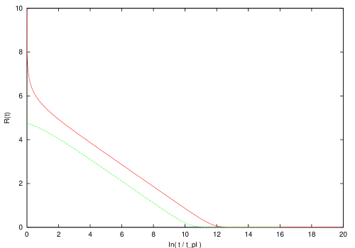
Figure 1: The evolution of $R$ is plotted for the analytic solution, equation (57), with dashed line (green) and the numerical one with a solid line (red).

This concludes the discussion on the background evolution. There is the possibility of extending the considerations by studying other potentials. Some qualitative aspects of these are covered in part in [26].

IV.2 Perturbation evolution during inflation

We turn now our attention to the consequences for cosmological perturbations generated during inflation. We will use the formalism discussed in [30], which is an extension of the formalism presented in [31]. We remind the reader again that we assume that $R$ does not play a role at least in the last 60 e–folds of inflation.

IV.2.1 Perturbation equations

The equations of motion for the fields $\Phi$ and $\chi$ are given by

$$\Box\Phi = \frac{1+2\alpha^{2}}{12\alpha^{2}}\left[A\frac{\partial A}{\partial\Phi}g^{\mu\nu}\partial_{\mu}\chi\partial_{\nu}\chi+\frac{\partial\tilde{V}}{\partial\Phi}\right].$$ (58)

$$\nabla_{\mu}\left[A^{2}g^{\mu\nu}\partial_{\nu}\chi\right] = \frac{\partial\tilde{V}}{\partial\chi}.$$ (59)

We now perturb the two fields

$$\Phi \rightarrow \Phi(t)+\delta\Phi(\mathbf{x},t),$$ (60)

$$\chi \rightarrow \chi(t)+\delta\chi(\mathbf{x},t).$$ (61)

Furthermore, we choose to work in the longitudinal gauge so that the perturbed metric looks like

$$ds^{2}=-(1+2\Psi)dt^{2}+a^{2}(1-2\Psi)d\mathbf{x}^{2}.$$ (62)

This generates the following equations of motion:

$$\delta\ddot{\Phi}+3H\delta\dot{\Phi}+\frac{k^{2}}{a^{2}}\delta\Phi = \frac{1+2\alpha^{2}}{12\alpha^{2}}\left[\left(\left(\frac{\partial A}{\partial\Phi}\right)^{2}\dot{\chi}^{2}+A\frac{\partial^{2}A}{\partial\Phi^{2}}\dot{\chi}^{2}\right)\delta\Phi\right.$$ (63)

$$\left.+2A\frac{\partial A}{\partial\Phi}\dot{\chi}\delta\dot{\chi}-\frac{\partial^{2}\tilde{V}}{\partial\Phi^{2}}\delta\Phi-\frac{\partial^{2}\tilde{V}}{\partial\Phi\partial\chi}\delta\chi\right]$$

$$-\frac{1+2\alpha^{2}}{6\alpha^{2}}\frac{\partial\tilde{V}}{\partial\Phi}\Psi+4\dot{\Phi}\dot{\Psi}.$$

$$A^{2}\left[\delta\ddot{\chi}+3H\delta\dot{\chi}+\frac{k^{2}}{a^{2}}\delta\chi\right] = \left[\frac{2}{A}\frac{\partial A}{\partial\Phi}\frac{\partial\tilde{V}}{\partial\chi}+2\left(\frac{\partial A}{\partial\Phi}\right)^{2}\dot{\chi}\dot{\Phi}-2A\frac{\partial^{2}A}{\partial\Phi^{2}}\dot{\chi}\dot{\Phi}\right]\delta\Phi$$ (64)

$$-\frac{\partial^{2}\tilde{V}}{\partial\chi^{2}}\delta\chi-\frac{\partial^{2}\tilde{V}}{\partial\chi\partial\Phi}\delta\Phi$$

$$-2A\frac{\partial A}{\partial\Phi}\left[\dot{\chi}\delta\dot{\Phi}+\dot{\Phi}\delta\dot{\chi}\right]$$

$$+4A^{2}\dot{\chi}\dot{\Psi}-2\frac{\partial\tilde{V}}{\partial\chi}\Psi.$$

This set up is equivalent to Di Marco et al [30] provided we make the field re–definition

$$\left(\frac{12\alpha^{2}}{1+2\alpha^{2}}\right)^{\frac{1}{2}}\Phi=\Sigma.$$ (65)

so that, dropping the tilde,

$$V(\Sigma,\chi) = V_{0}\chi^{n}\,e^{4\beta\Sigma},$$ (66)

$$\beta = \frac{-\alpha}{\sqrt{3}(1+2\alpha^{2})^{\frac{1}{2}}}$$ (67)

Once again note that $\alpha\rightarrow 0$ causes the modulus to decouple. We now define two new fields, the adiabatic and entropy perturbations, by

$$\delta\sigma = \cos\theta\delta\Sigma+A\sin\theta\delta\chi,$$ (68)

$$\delta s = -\sin\theta\delta\Sigma+A\cos\theta\delta\chi.$$ (69)

where

$$\cos\theta = \frac{\dot{\Sigma}}{\sqrt{\dot{\Sigma}^{2}+A^{2}\dot{\chi}^{2}}},$$ (70)

$$\sin\theta = \frac{A\dot{\chi}}{\sqrt{\dot{\Sigma}^{2}+A^{2}\dot{\chi}^{2}}}.$$ (71)

Furthermore, the gauge invariant curvature and entropy perturbations $\mathcal{R}$ (denoted as $\zeta$ in [30]) and $\mathcal{S}$ are defined as

$$\mathcal{R} = \Psi+H\left(\frac{\dot{\Sigma}\delta\Sigma+A^{2}\dot{\chi}\delta\chi}{\dot{\Sigma}^{2}+A^{2}\dot{\chi}^{2}}\right)=\Psi+H\frac{\delta\sigma}{\dot{\sigma}},$$ (72)

$$\mathcal{S} = H\left(\frac{A\dot{\Sigma}\delta\chi-A\dot{\chi}\delta\Sigma}{\dot{\Sigma}^{2}+A^{2}\dot{\chi}^{2}}\right)=H\frac{\delta s}{\dot{\sigma}},$$ (73)

where $\dot{\sigma}=\sqrt{\dot{\Sigma}^{2}+A^{2}\dot{\chi}^{2}}$. This demonstrates from where $\delta\sigma$ and $\delta s$ derive their names. In addition, the equation of motion for $\sigma$ is given by,

$$\ddot{\sigma}+3H\dot{\sigma} = -V_{\sigma},$$ (74)

$$V_{\sigma} = \cos\theta V_{\Sigma}+\frac{1}{A}\sin\theta V_{\chi}.$$ (75)

We are now able to write the perturbation equations in terms of the gauge–invariant variables. They are given by [30]:

$$\ddot{\mathcal{R}} + \left(3H-2\frac{\dot{H}}{H}+\frac{\ddot{H}}{\dot{H}}\right)\dot{\mathcal{R}}+\frac{k^{2}}{a^{2}}\mathcal{R}$$

$$= \frac{H}{\dot{\sigma}}\left[2(\dot{\theta}\delta s)^{.}-2\left(\frac{V_{\sigma}}{\dot{\sigma}}+\frac{\dot{H}}{H}\right)\dot{\theta}\delta s+2\beta h(t)\right].$$

$$\ddot{\delta s}+3H\dot{\delta s}+\left[\frac{k^{2}}{a^{2}}V_{ss}+3\dot{\theta}^{2}+\beta^{2}g(t)+\beta f(t)-4\frac{V_{s}^{2}}{\dot{\sigma}^{2}}\right]\delta s=2\frac{V_{s}}{H}\dot{\mathcal{R}}.$$ (77)

where

$$h(t) = \dot{\sigma}(\sin\theta\delta s)^{.}-\sin\theta\left[\frac{\dot{H}}{H}\dot{\sigma}+2V_{\sigma}-3H\dot{\sigma}\right]\delta s,$$ (78)

$$g(t) = -\dot{\sigma}^{2}(1+3\sin^{2}\theta),$$ (79)

$$f(t) = V_{\Sigma}(1+\sin^{2}\theta)-4V_{s}\sin\theta.$$ (80)

In addition we also define

$$V_{s} = -\sin\theta V_{\Sigma}+\frac{1}{A}\cos\theta V_{\chi},$$ (81)

$$V_{\sigma\sigma} = \cos^{2}\theta V_{\Sigma\Sigma}+\frac{2}{A}\cos\theta\sin\theta V_{\Sigma\chi}+\frac{1}{A^{2}}\sin^{2}\theta V_{\chi\chi},$$ (82)

$$V_{\sigma s} = \left(\frac{1}{A^{2}}V_{\chi\chi}-V_{\Sigma\Sigma}\right)\sin\theta\cos\theta+\frac{1}{A}V_{\Sigma\chi}\left(\cos^{2}\theta-\sin^{2}\theta\right),$$ (83)

$$V_{ss} = \sin^{2}\theta V_{\Sigma\Sigma}-\frac{2}{A}\cos\theta\sin\theta V_{\Sigma\chi}+\frac{1}{A^{2}}\cos^{2}\theta V_{\chi\chi}.$$ (84)

One is then able to see the coupling between the entropy and curvature perturbations. Note that whilst $V_{\sigma}=\frac{\partial V}{\partial\sigma}$ and $V_{s}=\frac{\partial V}{\partial s}$, it is not true that $V_{\sigma\sigma}=\frac{\partial^{2}V}{\partial\sigma^{2}}$ due to the dependence of the non–canonical kinetic term on $\Sigma$. The same holds for $V_{\sigma s}$ and $V_{ss}$. Normally, without the non–canonical kinetic term, one would find that there is no coupling if $\dot{\theta}=0$. We now see that, even if this holds, the coupling is maintained. Further, we see the manner in which the perturbations source one and other. In addition

$$\dot{\theta}=\dot{\sigma}\left[-\frac{V_{s}}{\dot{\sigma^{2}}}-\beta\sin\theta\right],$$ (85)

and so we see that the non–canonical kinetic term also introduces a source for $\theta$. This should be compared with the scenario in Randall–Sundrum where the entropy perturbations are generically suppressed due to the presence of the $\rho^{2}$ term in the Friedmann equation, [7]. Also, note that the parameter $\beta$ which describes the source from the non–canonical kinetic term, is constant in this setup. The next step is to examine the system numerically.

IV.2.2 Numerical Study of the Perturbation Spectra

The method for the evolution of the perturbations is as follows: we evolve the background staring with the initial conditions

$$\Sigma_{init} = 0,$$ (86)

$$\chi_{init} = 1000,$$ (87)

for $n\geq 0$. This means that at the beginning of inflation the inflaton mass will be equal to its physical one. When $-\dot{H}/H^{2}=1$, we stop the evolution as this is where the scale factor ceases to accelerate. We then backtrack 67 e–folds and switch on the perturbations where each mode starts inside the horizon with $k=1000aH$ at different times. With this prescription, the largest modes undergo 60 e–folds of inflation after horizon exit. We follow this evolution until the end of inflation.

To set the initial conditions one treats the modes, $\delta\sigma$ and $\delta s$, as independent stochastic variables deep inside the horizon. With this prescription, it can be shown that

$$a\delta\sigma=\frac{1}{\sqrt{2k}}e^{-\imath k\tau},$$ (88)

deep inside the horizon where the universe looks like Minkowski space. To calculate the spectra numerically, we use the method described in [32]. One makes two runs: the first run begins in the Bunch–Davis vacuum for $\delta\sigma$, $\delta s=\delta\dot{s}=0$, and the second in the Bunch–Davis vacuum for $\delta s$. The power spectra are then given by

$${\mathcal{P_{R}}} = \frac{k^{3}}{2\pi^{2}}\left(|{\mathcal{R}}_{1}|^{2}+|{\mathcal{R}}_{2}|^{2}\right),$$ (89)

$${\mathcal{P_{S}}} = \frac{k^{3}}{2\pi^{2}}\left(|{\mathcal{S}}_{1}|^{2}+|{\mathcal{S}}_{2}|^{2}\right),$$ (90)

$${\mathcal{P_{C}}} = \frac{k^{3}}{2\pi^{2}}|{\mathcal{R}}_{1}{\mathcal{S}}_{1}+{\mathcal{R}}_{2}{\mathcal{S}}_{2}|,$$ (91)

where the subscripts $1,2$ are the results for the two different runs. Furthermore, for the tensor modes, one finds

$$P_{\mathcal{T}}=8\left(\frac{H_{*}}{2\pi}\right)^{2},$$ (92)

we also define

$$r_{\mathcal{C}}=\frac{P_{\mathcal{C}}}{\sqrt{P_{\mathcal{R}}P_{\mathcal{S}}}},\ \ \ \ \ r_{\mathcal{T}}=\frac{P_{T}}{16P_{\mathcal{R}}}$$ (93)

Note that the definition for $r_{\mathcal{T}}$ is 16 times smaller than that used by the WMAP team, [33].

Figure 2: The evolution of the scalar perturbations for a given mode $k$ for the case $n=2$. We tune $V_{0}=10^{-10}$ to give the correct normalization for ${\mathcal{R}}$. This shows the 60 e–folds after horizon exit. Note that we plot $(P_{\mathcal{R}})^{\frac{1}{2}}$ and $(P_{\mathcal{S}})^{\frac{1}{2}}$.

If one examines the behavior of ${\mathcal{R}}$ and ${\mathcal{S}}$, we see that it is markedly different from the behavior observed in [26] where we have a run–away potential for $\chi$.

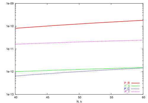
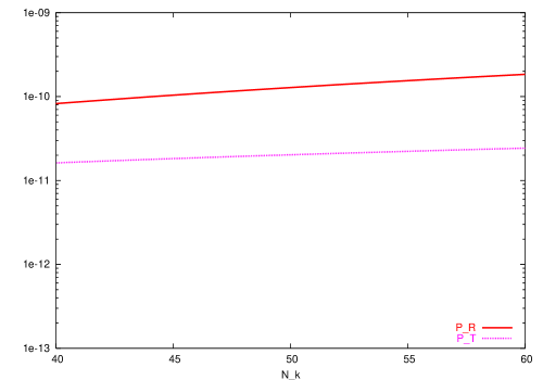
Figure 3: On the left we plot the spectra for the case $n=2$, $\alpha=0.01$ with $m_{\chi}\sim 10^{-5}$ ( $V_{0}=10^{-10}$ ). We see some running in the indices. In contrast, on the right we plot the same case with $\alpha=0$ with the amplitude of $P_{\mathcal{R}}$ scaled to coincide with the lefthand plot at $N_{k}=40$. This gives $m_{\chi}\sim 10^{-6}$. Note that there is no entropy production since we are effectively left with one field and, hence, there is also no correlation in this instance. We see that for this value of $\alpha$ there is very little difference between the plots for the curvature and tensor spectra.

Note that the mass required for the inflaton field is $m_{\chi}\sim 10^{-5}$ which is a few orders of magnitude heavier that one would normally use in the single field chaotic inflation model. This should not be surprising as the conformal factor decays during inflation and so reduces the effective mass of the inflaton.

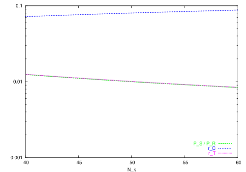
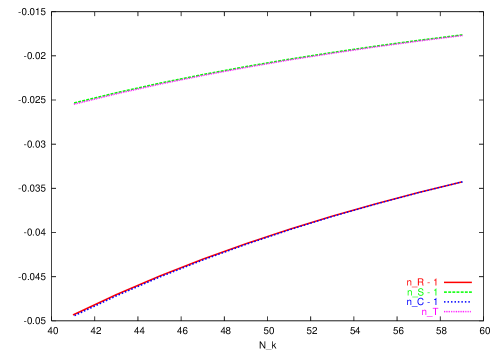
Figure 4: On the left we plot the evolution of the ratios for $n=2$, $\alpha=0.01$ and $V_{0}=10^{-10}$. Note that whilst the tensor production is small, the perturbations are quite well correlated. On the right we show the spectral indices. Here we see that the indices for entropy and tensor modes are coincident and similarly for the curvature and correlation.

Note that the tensor production is small but that there is a relatively large correlation between adiabatic and isocurvature modes. Furthermore we see some running of the indices but their overall values are consistent with the observations from WMAP. Note that the indices for entropy and tensor modes are coincident and similarly with the curvature and correlation. Finally, we find that the ratio ${\cal P}_{\cal S}/{\cal P}_{\cal R}$ is small, usually of order ${\cal O}(0.01)$.

Although observations demand that $\alpha\lesssim 10^{-2}$, it is possible to entertain larger values provided we stabilize the modulus $\Phi$ with some potential after the end of inflation. However, the smallness of the slow–roll parameter $\epsilon_{\Phi}$ ensures we must have

$$\alpha\ll\frac{1}{\sqrt{2}}.$$ (94)

to generate slow–roll inflation. One may then wonder what the effect of changing $\alpha$ has on the indices. For $n=2$, one can see that there is little effect for $\alpha\leq 10^{-2}$ but as it increases there is significant deviation from the single field case. In fact the largest possible value which generates enough inflation is $\alpha=0.25$ which produces $n_{\mathcal{R}}-1\approx-0.25$.

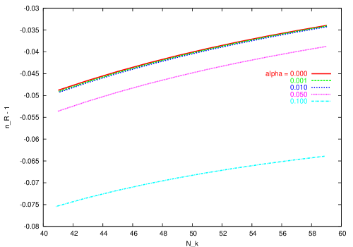
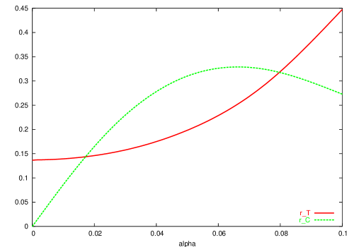
Figure 5: For the potential $V=\frac{1}{2}m_{\chi}^{2}\chi^{2}$, as we increase $\alpha$ we are drawn away from scale–invariance. Furthermore we see that this also leads to increased tensor production, scaled to agree with the normalization of WMAP. In addition it is possible to generate strong correlation between the perturbations.

This is not compatible with WMAP, [33], which constrains $\alpha\lesssim 0.2$. The reader is reminded that in the $\alpha\rightarrow 0$ limit the modulus $\Sigma$ decouples and we are left with a situation equivalent to the usual chaotic inflation [34].

Recent data from WMAP suggest that the quartic potential is under strong pressure. This very much depends on the number of e–folds we take as being observable and on the combination of data sets one uses [35]. Taking $N=60$, it is still permitted by the data. As this model is attractive from a particle physics point of view, we may wish to see if the coupling to the moduli helps to rule in or out this potential.

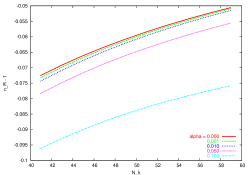
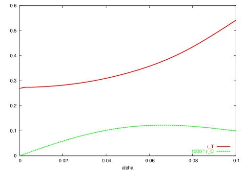
Figure 6: In left plot we see the effect of $\alpha$ on $n_{\mathcal{R}}$ for a potential of the form $V_{0}\chi^{4}$. One can immediately see that the results are similar for the chaotic inflation potential. Moreover, the increase in $\alpha$ also leads to an increase in the tensor modes, scaled to agree with the normalization of WMAP. The main difference is that these perturbations are effectively uncorrelated, $r_{\mathcal{C}}\sim 10^{-4}$.

One can immediately see from Figure 6 that the coupling to the moduli does us no favors. Increasing $\alpha$ produces more tensor modes– the main problem associated with $\chi^{4}$– and draws us further away from scale–invariance. A quick look at Figure 7 reveals that we are only just in the allowed region for $\alpha=0$. As in the case for the quadratic potential, the ratio ${\cal P}_{\cal S}/{\cal P}_{\cal R}$ is small.

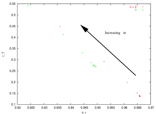
Figure 7: We see that the increase of $\alpha$ takes both models away from scale–invariance and leads to greater tensor production. This figure was generated with $V_{0}=10^{-10}$ for both sets of data but is independent of $V_{0}$.

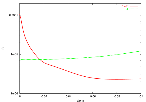
Figure 8: We examine the effect of $\alpha$ on the amplitude of the curvature perturbation. We see that for $n=2$ there is a significant effect. We have set $V_{0}=10^{-10}$ at $\alpha=0.01$ which gives $m_{\chi}\approx 10^{-5}$. Then we see that we get a range of $10^{-6}\leq m_{\chi}\leq 10^{-4}$ for $0\leq\alpha\leq 0.1$. For $n=4$, $\alpha$ has little effect of the amplitude of $\mathcal{R}$ where we set $V_{0}=10^{-15}$. We also see that reducing $\alpha$ increases the number of e–folds as one would expect since the potential becomes less steep.

V Conclusions

Boundary inflation in a brane world model with two boundary branes and a bulk scalar field was investigated. To study the system, we employed the low–energy effective action derived in [16]. Inflation, which must have happened at energies much lower than the brane tension if the four–dimensional theory is a good description, has some desirable features. In particular, the coupling to matter of one of the moduli fields (denoted $R$ in this paper) is driven towards small values. Therefore, if the inflationary epoch is long enough, the coupling of this field is very small after inflation and compatible with observations.

We found the background solutions for the fields and then studied the perturbation spectra numerically following the methods of [30]. We have seen that the effect of the coupling produces spectra which have indices smaller than one. Furthermore, the amplitude of tensor perturbations is enhanced compared to the predictions based on General Relativity. Our results imply that the mass of the inflaton for the quadratic potential can be larger than that normally required by the single field equivalent. In addition, the adiabatic and isocurvature perturbations can be highly correlated. In contrast, the quartic potential produces highly uncorrelated perturbations with the coupling having little effect on the required scale of the potential. Although this model is almost ruled out by current observations, one may have hoped that the coupling to the moduli may have helped its cause. We find this not to be the case and, in fact, the opposite is true. A large coupling would rule out this potential immediately.

Another feature discussed in this paper is that the negative tension brane collapses during inflation driven by a scalar field on the positive tension brane. Such behavior has already been observed in the matter–dominated era in [16]. This suggests that the five–dimensional spacetime is not stable during inflation (and matter domination) which is a fundamental problem of brane cosmologies based on models with bulk scalars. In the case of the Randall–Sundrum brane world with two branes, [24], the negative tension brane is driven towards the AdS horizon, whereas the positive tension brane would continue to inflate (and finally enter a radiation dominated phase). We would like to remind the reader that models based on string or M–theory motivate the existence of matter in the bulk (in particular scalar fields). Of course, the results presented in this paper will change dramatically once a potential for the fields $\Phi$ and $R$ is added. Such a potential could lead to the stabilization of the fields $\Phi$ and $R$ thereby avoiding the problem of the singularity. However, to derive a potential with cosmologically desirable properties is very difficult. In string theory, it is believed that such a potential can be derived once the non–perturbative sector of the theory is understood. Alternatively, string theory may naturally resolve the problem of the singularity. In our model, the underlying field theory has its limitations and the four–dimensional effective theory breaks down when $R$ approaches zero. In any case, it is clear that work has to be done to understand the behavior at $R=0$ better. For example, in [16] it was suggested that dark energy is related to this singularity problem. It would also be desirable to perform a calculation of the inflationary dynamics and the generation of perturbations in the full five–dimensional theory. However, the equations governing the perturbations are very difficult to solve.

Given the fact that models with non–canonical kinetic terms such as the one discussed in this paper arise in string theory, our results have an important impact on inflationary model building. At least for the potentials studied here, large couplings (i.e. of ${\cal O}(1)$) are not desirable.

Acknowledgements: We are grateful to R.H. Brandenberger and Ph. Brax for useful discussions. The authors are supported in part by PPARC.

1. V.A. Rubakov, Phys.Usp.44, 871 (2001)

2. Ph. Brax, C. van de Bruck, Class.Quant.Grav.20, R201 (2003)

3. D. Langlois, Prog.Theor.Phys.Suppl.148 181 (2003)

4. R. Maartens, D. Wands, B.A. Bassett, I. Heard, Phys.Rev.D 62, 041301 (2000)

5. D. Langlois, R. Maartens, D. Wands, Phys.Lett.B 489, 259 (2000)

6. E.J. Copeland, A.R. Liddle, J.E. Lidsey, Phys.Rev.D 64, 023509 (2001)

7. P.R. Ashcroft, C. van de Bruck, A.C. Davis, Phys. Rev. D. 66, 121302 (2002)

8. G. Huey, J.E. Lidsey, Phys.Rev.D 66, 043514 (2002)

9. A.R. Liddle, A.J. Smith, Phys.Rev.D 68, 061301 (2003)

10. E. Ramirez, A.R. Liddle, astro-ph/0309608

11. Y. Himemoto, T. Tanaka, M. Sasaki, Phys.Rev.D 65, 104020 (2002)

12. R.M. Hawkins, J.E. Lidsey, astro-ph/0306311

13. D. Seery, A. Taylor, astro-ph/0309512

14. A. Linde, Particle Physics and Inflationary Cosmology, Harwood Academic Publishers (1990)

15. A.R. Liddle, D.H. Lyth, Cosmological Inflation and Large–Scale Structure, Cambridge University Press (2000)

16. Ph. Brax, C van de Bruck, A.-C. Davis, C.S. Rhodes, Phys.Rev.D. 67,023512 (2003)

17. J. Garriga, O. Pujolas, T. Tanaka, Nucl.Phys. B 655, 127 (2003)

18. T. Damour, G. Esposito-Farese, CQG 9 2093 (2001)

19. C.S. Rhodes, C. van de Bruck, Ph. Brax, A.-C. Davis, astro-ph/0306343

20. J. Martin, R. H. Brandenberger, Phys.Rev.D63,123501 (2001)

21. J. Garcia-Bellido, D. Wands, Phys.Rev.D 52, 5636 (1995)

22. J. Garcia-Bellido, D. Wands, Phys.Rev.D 52, 6739 (1995)

23. T. Damour, A. Vilenkin, Phys.Rev.D 53, 2981 (1996)

24. L. Randall, R. Sundrum, Phys. Rev. Lett.83, 3370 (1999)

25. Ph. Brax, A.-C. Davis Phys. Lett. B 497, 289 (2001)

26. P.R. Ashcroft, C. van de Bruck, A.C. Davis, astro-ph/0210597

27. S. Kobayashi, K. Koyama, JHEP 0212, 056 (2002)

28. A. Lukas, B.A. Ovrut, D. Waldram, Phys.Rev.D 61, 023506 (2000)

29. A.V. Frolov, L. Kofman, hep-th/0309002

30. F. Di Marco, F. Finelli, R. Brandenberger, Phys.Rev.D 67, 063512 (2003)

31. C. Gordon, D. Wands, B.A. Bassett, R. Maartens, Phys.Rev.D 63, 023506 (2001)

32. S. Tsujikawa, D. Parkinson, B.A. Bassett,Phys. Rev.D67 083516 (2003)

33. H. V. Peiris et al, Astrophys.J.Suppl. 148, 213 (2003)

34. A. Linde,Phys. Lett.B 129 177 (1983)

35. W. Kinney, E. Kolb, A. Melchiorri,A.Riotto, astro-ph/0305130