Possibility of a White Dwarf as the Accreting Compact Star
in CI Cam ( = XTE J0421+560)

Abstract

We present results from ASCA observations of the binary CI Cam both in quiescence and in outburst in order to identify its central accreting object. The quiescence spectrum of CI Cam consists of soft and hard components which are separated clearly at aound 2–3 keV. A large equivalent width of an iron K$\alpha$ emission line prefers an optically thin thermal plasma emission model to a non-thermal power-law model for the hard component, which favors a white dwarf as the accreting object, since the optically thin thermal hard X-ray emission is a common characteristic among cataclysmic variables (binaries including an accreting white dwarf). However, since the power-law model, which represents the X-ray spectrum of the soft X-ray transients in quiescence, provides with an equally good fit to the hard component statistically, we cannot exclude possibilities of a neutron star or a black hole from the quiescence data.

The outburst spectrum, on the other hand, is composed of a hard component represented by a multi-temperature optically thin thermal plasma emission and of an independent soft X-ray component that appears below 1 keV intermittently on a decaying light curve of the hard component. The spectrum of the soft component is represented well by a blackbody with the temperature of $0.07-0.12$ keV overlaid with several K-edges associated with highly ionized oxygen. This, together with the luminosity as high as $\sim 1\times 10^{38}{\rm erg\;s}^{-1}$, is similar to a super-soft source (SSS). The outburst in the hard X-ray band followed by the appearance of the soft blackbody component reminds us of recent observations of novae in outburst. We thus assume the outburst of CI Cam is that of a nova, and obtain the distance to CI Cam to be 5–17 kpc by means of the relation between the optical decay time and the absolute magnitude. This agrees well with a recent estimate of the distance of 5–9 kpc in the optical band. All of these results from the outburst data prefer a white dwarf for the central object of CI Cam.

1 Introduction

On 1998 Mar 31 Smith et al. (1998) discovered the new X-ray transient XTE J0421+560 with the All-Sky Monitor (ASM; Levine et al. (1996)) on board Rossi X-ray Timing Explorer (RXTE). Follow-up observations of the ASM and the Proportional Counter Array (PCA) showed that XTE J0421+560 reached its peak intensity of $\sim$2 Crab on Apr 1.04, well within a day from the onset of the outburst. On Apr 2.63, Hjellming & Mioduszewski (1998a) found a variable radio source within the PCA error circle (Marshall, Strohmayer, & Lewin, 1998). The position of the radio source coincides with that of the optical variable star CI Cam (Wagner & Starrfield, 1998), which establishes CI Cam being the optical counterpart of XTE J0421+560.

The observations of BeppoSAX on Apr 3 and 9 and of ASCA on Apr 3-4 revealed that, unlike the other X-ray transients which harbor a black hole (BH) or a neutron star (NS) (Tanaka & Shibazaki, 1996), the X-ray spectra up to 10 keV have optically thin thermal nature with a plenty of K-shell emission lines from highly ionized O, Ne, Si, S, and Fe (Frontera et al., 1998; Orr et al., 1998; Ueda et al., 1998). The spectra can be represented well by a two temperature optically thin thermal plasma emission model with the temperatures of ${}^{<}_{\sim}$ 1 keV and 3–6 keV. Significant cooling of the plasma and the intensity declination were found both between the two BeppoSAX observations and within the single ASCA observation. From a detailed X-ray temporal analysis based on the PCA data during the outburst was found no rapid random variability (Belloni et al., 1999), which is remarkably different from the NS and BH transients. The X-ray to radio light curves (Frontera et al., 1998) clearly show that the burst peak occurs later for longer wavelengths, and the $e$-folding decay time is shorter for shorter wavelengths. The Burst and Transient Source Experiment (BATSE) on board Compton Gamma Ray Observatory (CGRO) recorded the shortest timescales among all of the wavebands, the intensity arriving at the peak within only $\sim$ 0.1 d and its $e$-folding decay time being $\sim$ 0.56 d (Harmon, Fishman, & Paciesas, 1998). The hard X-ray spectrum in the band 20–100 keV obtained with the BATSE between Apr. 1.0–2.0 is represented by a power law with a photon index of $3.9\pm 0.3$. The flux is compatible with that of the contemporaneous RXTE PCA observations in the band 2–25 keV (Belloni et al., 1999). In the optical spectra, a broad blue wing with the velocity of more than 2500 km s^-1 was detected from hydrogen Balmar emission lines only during the outburst (Robinson, Ivans, & Welsh, 2002; Hynes et al., 2002). By comparing the radio data on Apr 2.63 and 3.83, Hjellming & Mioduszewski (1998b) found that the radio spectra showed a transition from optically thick to thin. The results described described above indicate that the radiation from radio to $\gamma$-ray during the outburst originates from an expanding gas ejected by a sort of eruptive event.

Observations of XTE J0421+560 in quiescent state, on the other hand, were carried out by BeppoSAX in 1998 September (Orlandini et al., 2000), 1999 September and 2000 February (Parmar et al., 2000), and by XMM-Newton in 2001 August (Boirin et al., 2002). Except for the third BeppoSAX observation only giving an upper limit to the absorption-corrected 1–10 keV luminosity of $<2.5\times 10^{33}$ erg s^-1, the other three observations positively detected XTE J0421+560 at the luminosities in the range $(1.4-23)\times 10^{33}$ erg s^-1. The X-ray spectrum obtained by XMM-Newton is likely to be composed of two components; one dominates in the band below $\sim$ 4 keV with little absorption, and the other, undergoing heavy photoelectric absorption with $N_{\rm H}=5^{+3}_{-2}\times 10^{23}$ cm^-2, is conspicuous above $\sim$ 5 keV. It seems that the spectrum of the first BeppoSAX observation is dominated by the former component, whereas that of the second is so by the latter. It is worth noting that a strong iron emission line centered at $6.43\pm 0.09$ keV is detected in the XMM-Newton observation with the equivalent width of $940^{+650}_{-460}$ eV. An emission line, probably attributable to iron, is also detected at $7.0^{+1.6}_{-0.2}$ keV and $7.3\pm 0.2$ keV, respectively, from the first and second BeppoSAX observations (Orlandini et al., 2000; Parmar et al., 2000).

The optical nature of CI Cam had been a matter of debate until recently. It was originally designated as MWC 84 in a list of Be stars with infrared excess (Allen & Swings, 1976) which are later recognized as B[e] stars. Although a symbiotic characteristic is reported (Bergner et al., 1995), Belloni et al. (1999) argued against this based on their infrared to optical spectrum, and claimed it to be classified as a B[e] star. Taking into account the high bolometric luminosity and composition of the optical emission lines, Robinson, Ivans, & Welsh (2002) finally categorized CI Cam into a supergiant B[e] (sgB[e]) star, which has prodigious mass loss rate $>10^{-5}M_{\odot}$ yr^-1 (de Freitas Pacheco et al., 1998) and high bolometric luminosity $10^{5}<L_{\rm bol}/L_{\odot}<10^{6}$ (Zickgraf, 1998).

The distance to CI Cam had been estimated to be $1-2$ kpc based on the luminosity, and the extinction-distance relation (Zorec, 1998; Belloni et al., 1999; Clark et al., 2000; Orlandini et al., 2000). Robinson, Ivans, & Welsh (2002), however, pointed out that the extinction-distance relation is unreliable in the direction of CI Cam, because the interstellar matter is patchy. They proposed a new distance estimate based on the velocity of optical emission lines with the aid of the Galactic rotation model (Burton, 1988a), distribution of matter in the Galactic disk (Burton, 1988b), and distances to the known H II region (Blitz, Fich & Stark, 1982; Chan & Fich, 1995). Hynes et al. (2002) also estimated the distance by making use of a velocity structure of the interstellar Na D absorption line. The authors of these two papers arrived at almost the same conclusion that the distance to CI Cam is in the range 5–9 kpc. We hereafter adopt the distance of 5 kpc as a default according to recent convention.

One of the most controversial issues as yet unsettled for CI Cam is the identification of the accreting compact object. There are, of course, three possibilities: either a BH, a NS, or a white dwarf (WD). Orlandini et al. (2000) pointed out that the outburst behavior of CI Cam is similar to nova outburst, and that the compact object might be a WD. Belloni et al. (1999) argued for a NS since the overall outburst behavior is similar to that of the 69 ms X-ray pulsar A0538$-$66 in LMC (Corbet et al., 1997). Robinson, Ivans, & Welsh (2002) obtained the X-ray luminosity of $L(2-25\mbox{ keV})=3\times 10^{38}$ erg s^-1 based on their revised distance of 5 kpc, making CI Cam one of the most luminous X-ray transient. Comparing the outburst luminosity to that during quiescence, they concluded that the compact object is most likely a BH.

In this paper, we present results from ASCA observations of CI Cam in quiescence and those from more detailed analysis of the soft X-ray component in outburst dominating below $\sim$ 1 keV (Ueda et al., 1998), which is probably identical with that detected in one of the 1998 Apr observations by BeppoSAX (Orr et al., 1998). Overall X-ray behavior revealed by the ASCA observations is consistent with the picture that the compact object in CI Cam is a WD, and the eruptive event that triggers the hard X-ray outburst can be identified with a nova outburst (= thermonuclear flash on the surface of the WD). We note that the errors quoted throughout this paper are those at the 90 % confidence level, unless mentioned otherwise.

2 Observations

The ASCA observation of CI Cam in quiescence was performed during 1999 Feb 19.415-20.445, which was between the first (1998 Sep 3-4) and second (1999 Sep 23-35) BeppoSAX observations of CI Cam in quiescence (Orlandini et al., 2000; Parmar et al., 2000). Throughout the observation, Solid-state Imaging Spectrometer (SIS; Burke et al. (1994); Yamashita et al. (1999)) was operated in 1-CCD Faint mode, and Gas Imaging Spectrometer (GIS; Ohashi et al. (1996); Makishima et al. (1996)) was so in PH mode with the default telemetry bit assignment. We retrieved the data from the Data ARchive and Transmission System (DARTS) operated in the Institute of Space and Astronautical Science (ISAS).

We applied the following selection criteria to both the SIS and GIS data. We did not use the data while the spacecraft locates within 60 s from the South Atlantic Anomaly. We also discarded the data while the pointing direction of the telescope was within 5 deg from the Earth limb. In addition to these, we further adopted the following two criteria only for the SIS. We discarded the data while the pointing direction of the telescope was within 20 deg from the edge of the bright Earth limb illuminated by the Sun. After these criteria being applied, some 37.4 ks and 43.8 ks remain as the good time intervals for the SIS and the GIS, respectively. For source photon integration regions, we adopted a circle with a radius of 2 arcmin and 3 arcmin centered on CI Cam for the SIS and the GIS, respectively. For background regions, we used the residual area of the same CCD chip employed for the CI Cam observation that is out of the source integration region for the SIS, while, for the GIS, we adopted a circle with a radius of 6 arcmin whose center locates opposite to the source integration region with respect to the optical axis of the telescope, in order to take vignetting of the telescope into account. After background subtraction, the average count rates throughout the observation are $0.054\pm 0.003$ and $0.058\pm 0.004$ c s^-1 per detector for the SIS in the band 0.5–10 keV and the GIS in the band 0.7–10 keV, respectively.

The ASCA observation of CI Cam in outburst was carried out from 1998 Apr 3.31 to 4.14, which was only three days after the onset of the outburst, and only two days after the X-ray peak (Smith et al., 1998). Detailed observation journal was described in Ueda et al. (1998). The spectrum was represented by the two temperature optically thin thermal emission model with temperatures of 1.1 keV and 5.7 keV with relative abundances of Si, S, and the other metals being 1.25$\pm$0.04, 1.03$\pm$0.13, and 0.36$\pm$0.02, respectively, relative to the cosmic composition (Anders & Grevesse, 1989). A neutral iron emission line at 6.41 keV was found with an equivalent width of 90 eV. The entire spectrum was covered by neutral absorber with $N_{\rm H}=(4.6\pm 0.3)\times 10^{21}$ cm^-2. In addition to this hard X-ray component, they also discovered the other spectral component which appears and flickers in the latter half of the observation. Its spectrum has a sharp cutoff at $\sim 0.8$ keV, and only detected below 0.9 keV (Ueda et al., 1998). They could fit the spectrum with a blackbody model with $kT=0.12\pm 0.02$ keV with K-edges of hydrogenic and He-like oxygen at $\sim$0.77 keV and $\sim$0.84 keV. We are interested in this soft component, which is not analyzed in full detail by Ueda et al. (1998). Accordingly, we concentrate on the SIS in analyzing the outburst data, because the SIS has higher sensitivity below 1 keV than the GIS. The same selection criteria as those for the quiescence data are applied, except that the radius of the source photon integration region is taken to be 3 arcmin.

3 Analysis and Results

3.1 Light Curve in Quiescence

We have first made light curves of CI Cam in quiescence, in order to see if there is any variability during the ASCA observation. According to the data selection criteria (§ 2), we have extracted source and background photons for each detector (SIS0, SIS1, GIS2, GIS3) separately. With a bin width of 6400 s, we have created light curves of the SIS by adding up the photons from the two SIS detectors after background subtraction. The same procedure is applied for the GIS. The large bin size of 6400 s is adopted because of statistical limitation. As shown in the next subsection, the ASCA spectrum (Figure 1) and also the XMM-Newton spectrum (Boirin et al., 2002) both in quiescence obviously consist of two spectral components separated at around a few keV. Accordingly, the light curves are made in the two bands 0.5–2.0 keV (soft) and 2.0–7.0 keV (hard) as well as 0.5–7.0 keV (total) for the SIS, and 0.7–2.0 keV (soft), 2.0–7.0 keV (hard) and 0.7–7.0 keV (total) for the GIS. In order to improve statistics, we have further summed up the SIS and GIS light curves in the corresponding bands, and then have fitted them with a constant model. The resultant $\chi^{2}_{\nu}$ (d.o.f.) is 0.65 (13), 1.10 (13), and 1.46 (13) for the soft, hard, and total light curves, respectively. Although one can find that both the soft and hard components are variable in a longer timescale by comparing the three BeppoSAX observations (Orlandini et al., 2000; Parmar et al., 2000) and the observation of XMM-Newton (Boirin et al., 2002), their fluxes are consistent with being constant within the single ASCA observation on a timescale between $\sim$2 h and 1 d.

3.2 Spectrum in Quiescence

Since there is no evidence for variability, we evaluate the spectra averaged throughout the observation, which are shown in Figure 1 for the SIS and the GIS separately. As obviously seen, they are composed of the two continuum components separated at 2–3 keV. Accordingly, we have attempted to fit them with soft and hard components undergoing independent photoelectric absorptions. For spectral fitting, we use XSPEC v11.2 (Arnaud, 1996). Throughout this subsection, the GIS and SIS spectra are always fitted contemporaneously.

First of all, we have attempted to fix spectral models for both emission components from a purely statistical point of view. We have tried optically thin thermal plasma emission (mekal), power law, and blackbody models for the soft component, and mekal, power law, and thermal bremsstrahlung models for the hard component. As noticed from Figure 1, the ASCA spectra suggest presence of an iron K$\alpha$ emission line feature around 6-7 keV. The iron K$\alpha$ emission lines have also been detected from the BeppoSAX and XMM-Newton observations (Parmar et al., 2000; Boirin et al., 2002). We thus have added a narrow Gaussian, with its central energy free to vary, in the case that either the power law or the thermal bremsstrahlung is adopted for the hard component. In order to check the validity of adding the Gaussian line, we have tried a model composed of a soft mekal and a hard power law, and by including a Gaussian, we have found that the resultant $\chi^{2}$ value is improved from 38.23 (44 d.o.f.) to 31.78 (42 d.o.f.), implying $\Delta\chi^{2}=6.46$ for 2 degrees of freedom. According to F-test, the inclusion of the iron line into the ASCA spectra is justified at the $98.0$ % confidence level.

The best-fit $\chi^{2}_{\nu}$ matrix for the fits with the trial models is summarized in Table 1. There is no reason to prefer any particular model statistically for both soft and hard components. We thus need some physical consideration in choosing a particular pair of the models. It has been suggested that the soft component probably originates from the sgB[e] star (Robinson, Ivans, & Welsh, 2002). The temperature of $\sim 0.22$ keV (Orlandini et al., 2000) and the 0.5-2.0 keV luminosity of $2\times 10^{34}$ erg s^-1 is consistent with the X-ray emission from sgB[e] star (Robinson, Ivans, & Welsh, 2002). The power-law fit to the soft band spectrum of the current ASCA data results in the photon index of $5.3^{+1.8}_{-1.1}$. Such a steep spectrum probably corresponds to a high energy end of a thermal spectrum. Accordingly, we hereafter adopt the mekal model for the soft component.

For the hard component, on the other hand, since the mekal model and the thermal bremsstrahlung plus Gaussian model are essentially the same, we compare the power-law model (plus Gaussian) with the mekal model. The results of the fits in the band 0.5-10 keV, including the soft mekal below $\sim 2$ keV, are summarized in Table 2. For the mekal components, we have first tried to set their abundances free to vary independently. (“2 mekal I” model in Table 2), and have found that they become consistent within the errors. We thus have constrained the two abundances to be the same (“2 mekal II” model). The fit with this model results in the abundance to be $0.26^{+0.54}_{-0.26}$ times the cosmic value (Anders & Grevesse, 1989). The error is, however, large due to statistical limitation. We thus have fixed them at the value 0.36 times the cosmic obtained from the outburst observation by Ueda et al. (1998) (“2 mekal III” model). As can be seen from Table 2, all of the three mekal fits are acceptable at the 90 % confidence level, and the fit with “2 mekal I” model is formally the best. As described above, however, the soft component can be interpreted as the coronal emission from the sgB[e] star, and since the hard component emission is probably a result of mass accretion from the sgB[e] star, there is no reason that the abundance of the hard mekal component is different from that of the soft. Accordingly, we believe the last “2 mekal III” model is physically most reasonable. Based on this model, the best-fit temperatures of the soft and hard components are obtained to be $kT_{1}=0.45^{+0.17}_{-0.14}$ keV and $kT_{2}=5.5^{+7.7}_{-2.9}$ keV, respectively. Bolometric luminosities of the hard mekal component is calculated from the emissivity of thermal bremsstrahlung (Rybicki & Lightman, 1979) at the observed temperature and the emission measure. Those of the soft mekal, on the other hand, is calculated from the emissivity of the optically thin thermal plasma (Gaetz & Salpeter, 1983). Around the plasma temperature of $0.4-0.5$ keV observed, the emissivity of the plasma is dominated by the iron L line emissions. Accordingly, we have reflected the observed iron abundance into the luminosity calculation. As a result, the bolometric luminosities of the soft and hard components based on “2 mekal III” model are obtained to be $6.0\times 10^{33}$ erg s^-1 and $9.4\times 10^{33}$ erg s^-1, respectively.

The power-law model, on the other hand, can fit the spectra equally well as the mekal models. We thus next consider the non-thermal power law as the continuum emission model of CI Cam in quiescence. In this case, the observed iron emission line should be of fluorescence origin. We assume that the line originates from matter surrounding the hard component emitter uniformly with the $4\pi$ solid angle. The thickness of the matter is then equal to the line of sight photoelectric absorption $N_{\rm H2}=1.9^{+0.4}_{-0.2}\times 10^{23}$ cm^-2 (Table 2). From this hydrogen column density, the equivalent width of the iron K$\alpha$ emission line is expected to be $190^{+40}_{-20}$ eV under the condition that the intrinsic photon index of a power-law emission is 1.1 and that the fluorescing matter has the cosmic composition (Inoue, 1985). In the case of CI Cam, there are two factors to reduce the expected equivalent width; one is the iron abundance, which is 0.36$\pm$0.02 times the cosmic (Ueda et al., 1998), that reduces the equivalent width proportionally; the other is the larger photon index of 2.28 (Table 2), which also reduces the equivalent width according to the following scaling relation;

$$EW(\gamma)\;\propto\;\frac{1}{f(E_{\rm K\alpha};\gamma)}\int^{\infty}_{E_{\rm edge}}f(E;\gamma)\;\sigma(E;E_{\rm edge})\;dE$$

(Ezuka & Ishida, 1999), where $f(E_{\rm K\alpha};\gamma)$ represents the intrinsic X-ray photon flux density of the power law with the photon index $\gamma$ at the energy $E_{\rm K\alpha}$, and $E_{\rm K\alpha}$ and $E_{\rm edge}$ are the energies of the K$\alpha$ line and the K-edge of the neutral iron, which are 6.40 keV and 7.11 keV, respectively. $\sigma$ is the cross section of the iron K-edge photoelectric absorption. In the case of $\gamma=2.28$, we have obtained the $EW$-scaling factor from the $\gamma=1.1$ case to be 0.64, assuming $\sigma(E;E_{\rm edge})\propto E^{-3}$ for $E>E_{\rm edge}$. As a result, the expected equivalent width from CI Cam becomes only $\sim$40 eV with the 90%upper limit of $80$ eV within the errors of the related parameters. This cannot be compatible with the observed equivalent width of $624^{+418}_{-495}$ eV (Table 2). It seems that the observed iron K$\alpha$ emission line is difficult to be explained solely by the fluorescence, and that the underlying continuum is likely to be the optically thin thermal plasma emission, supplying additional iron K$\alpha$ line emission. In Figure 1, we show the best-fit “2 mekal III” model by histograms, which we put forward as the best representation of the CI Cam spectra. We note, however, that this conclusion is derived under the hypothesis of the fluorescing matter surrounding the central object uniformly. This may, however, not be true, because there is a dense circumstellar disk around the sgB[e] star out of the line of sight. Also the absorber is assumed to be neutral, but this may not be true, either. Both these effects provide with a larger equivalent width at a given line of sight column density estimated with neutral matter cross section. Hence, we cannot rule out the power-law model for the hard spectral component of CI Cam in quiescence.

Note also that, although we have shown that the thermal iron K$\alpha$ line is preferred, partial contribution of the fluorescent component is not ruled out. In the XMM-Newton observation (Boirin et al., 2002), the iron line is detected at the energy $6.43\pm 0.09$ keV with the equivalent width of $940^{+650}_{-460}$ eV, which is greater than that obtained with ASCA. Since the line of sight hydrogen column density during the XMM-Newton observation is also greater than during the ASCA observation, the greater equivalent width and the lower line central energy are probably brought about by the increment of the contribution of the fluorescent component. The upper limit of the line width 0.28 keV obtained by XMM-Newton probably allows contribution from the thermal plasma component to the observed iron line. Hence, the iron K$\alpha$ emission line from CI Cam is probably a mixture of the thermal plasma and fluorescent components. For the ASCA spectra in Figure 1, it is possible to insert an additional Gaussian representing the fluorescent iron line into the model, which we have, however, refrained from because of statistical limitation.

3.3 Reanalysis of the Soft Component in the Outburst Spectrum

3.3.1 Light curve

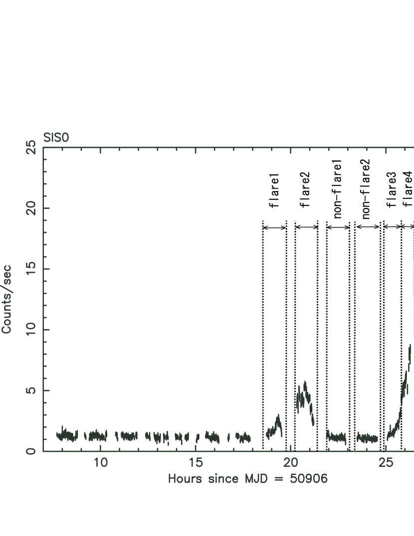
Figure 2: The SIS0 light curve of CI Cam in the band 0.5–1.0 keV during the outburst.

As described in § 1, the X-ray emission from CI Cam during the outburst is dominated by that from the optically thin thermal plasma with a temperature of several keV (Ueda et al., 1998), which is probably escaping from the binary system. In addition to this, a separate soft X-ray component that is detected only below 1 keV starts to appear in the middle of the ASCA observation. Although it once fades away, it brightens again nearly the end of the observation. We show the SIS0 light curve during the outburst in Figure 2. As noted by Ueda et al. (1998), the satellite telemetry is saturated after around Apr. 4 2:40 due to the increasing intensity of the soft component, and the detection efficiency of the SIS at the image core is significantly reduced as a result of event pile-up. We have corrected this effect by utilizing photons well outside the overflowed core and a saturated region in drawing the light curve.

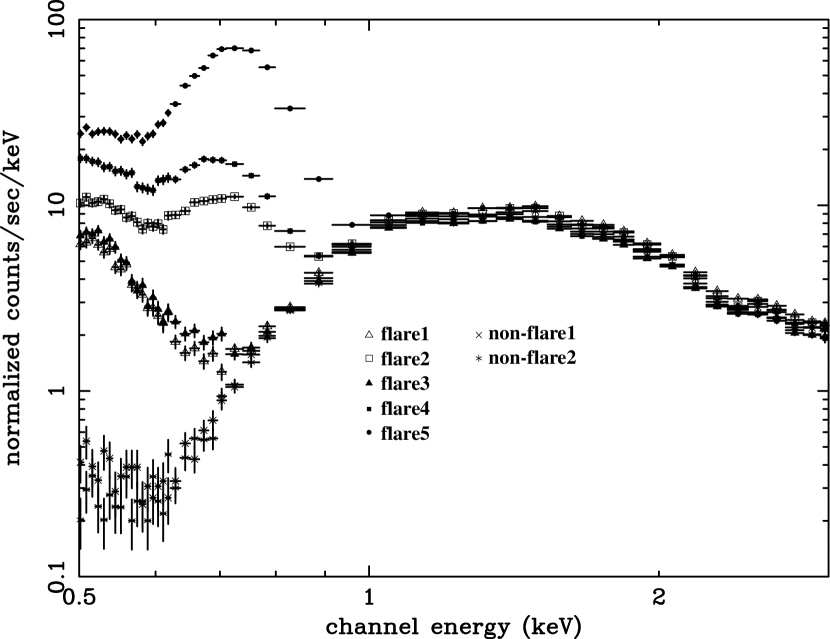
Figure 3: The SIS0+SIS1 spectra of CI Cam from the segments “flare 1–5” and “non-flare 1 & 2” in Figure 2.

In order to examine the nature of the soft component, we have divided the full dataset into several pieces designated as “flare 1 & 2”, “non-flare 1 &2” and “flare 3–5” in Figure 2, as delineated by the dashed vertical lines, and have drawn the average SIS spectra during those intervals separately, which are shown in Figure 3. We have corrected the event pile-up effect for the spectrum during the “flare 5” interval. As obviously seen from the spectral variation, what changes during the soft flare is not the line of sight absorption but the emission component itself; the spectrum extends to a higher energy band as the intensity increases. Owing to a very slow decay of the hard component, the flux levels of all of the data segments are similar above $\sim$1 keV. Accordingly, we regard the average of “non-flare 1 & 2” spectra as the background and simply subtracted them from the “flare” spectra.

3.3.2 Evaluation of the Spectra by a Power Law

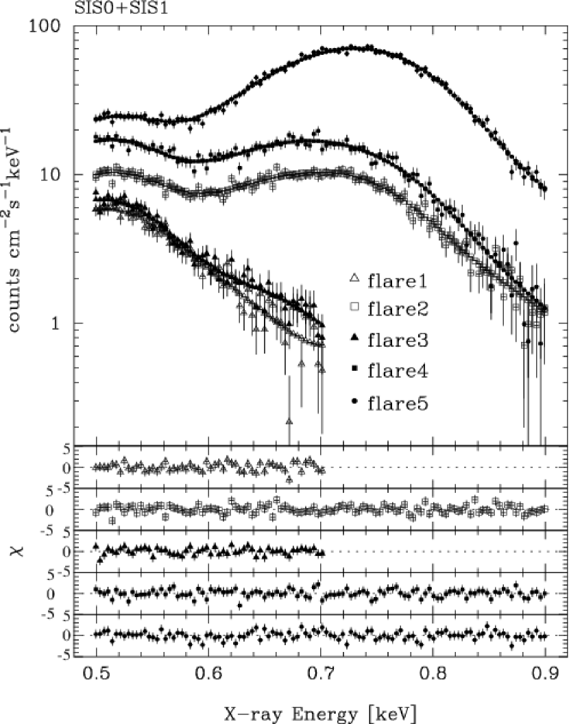
Figure 4: The best-fit SIS0+SIS1 spectra of CI Cam from the segments “flare 1–5” fitted by the blackbody with the five oxygen edges. The top panel shows the data and the models for the five “flare” spectra. The other five panels below show the fit residuals for the five spectra separately. For the best-fit parameters, see Table 5.

We have first tried to fit all five flare spectra after the background subtraction (Figure 4) by a power law undergoing the photoelectric absorption. We have used the spectral energy bins in the band 0.5–0.7 keV for “flare 1 & 3”, and 0.5–0.9 keV for the others. The fits are, however, generally poor. Ueda et al. (1998) pointed out that the high energy cutoff starting at $\sim$0.8 keV seen in the “flare 5” spectrum is as steep as what can only be realized by a sharp atomic edge. According to them, we have overlaid the power law with two edges, and have tried to fit the spectra again. In doing this, we have fixed the hydrogen column density at $4.6\times 10^{21}{\rm cm}^{-2}$, which is obtained by the fit to the hard X-ray component during outburst out of the soft flare (Ueda et al., 1998). The results are summarized in Table 3. The fits for all five spectra are markedly improved and now acceptable at the 90 % confidence level. Although the power-law model is acceptable as an underlying continuum, however, it is difficult to understand the large variation of the photon index ranging 0.5–5.3 over the five flare phases. No power-law X-ray source has been known so far whose photon index varies in such a wide range on the timescale of a day. The apparent large photon index variation thus probably represents a temperature variation of the continuum. We therefore examine a blackbody model in the following subsection.

3.3.3 Evaluation of the Spectra by a Blackbody

We have attempted to fit all of the 5 flare spectra with the blackbody model in the same energy bands as in the previous subsection. As we already know, some absorption edges are necessary to fit the spectra. We thus have introduced the absorption edges one by one until we obtain acceptable $\chi^{2}$ values. The results are summarized in Table 4. As suggested by Figure 3, the blackbody temperature increases with the intensity whereas no $N_{\rm H}$ decrease is found with increasing intensity. Two edges are necessary to fit the “flare 2, 4 & 5” spectra, one edge for the “flare 1” spectrum, and no edge for the “flare 3 ” spectrum. The fit to the “flare 3” spectrum is, however, further improved significantly if we overlay the blackbody with an edge at 0.67 keV, as listed in the last column of Table 4. Note that the obtained edge energies in the “flare 1 & 3” spectra (0.62 keV and 0.67 keV, respectively) are somewhat apart from those of O VII and O VIII K-edges. Obviously we need a more systematic and sophisticated treatment for the oxygen edges, which is essential to determine the intrinsic spectral shape and the luminosity of the soft component.

In the second column of Table 5, we have tabulated the energies of ionized oxygen edges above 0.60 keV (Verner & Yakovlev, 1995). It is likely that the edges found in the “flare 1 & 3” spectra are associated with O IV or O V. We thus have introduced a model composed of a blackbody with five edges corresponding to O IV through O VIII. If we allow all of their energies to vary independently, however, they never converge because of the limited energy resolution and the narrow energy bands available. We have therefore linked the energies $E_{\rm edge\,2}$ through $E_{\rm edge\,5}$ to $E_{\rm edge\,1}$ so that their ratios to $E_{\rm edge\,1}$ are consistent with the theoretical values listed in the second column of Table 5. The results of the best-fit to each “flare” spectrum are shown in Figure 4, whose parameters are listed from the third column in Table 5, where $\tau_{1}$ through $\tau_{5}$ are the optical depths of the edges at their threshold energies. We have multiplied the model by the photoelectric absorption of the cosmic composition with the fixed hydrogen column density of $4.6\times 10^{21}{\rm cm}^{-2}$, which is obtained from the same outburst observation while the soft component is absent (Ueda et al., 1998). In addition to this, we have also overlaid an additional photoelectric absorption with a free $N_{\rm H}$, in order to see if there is excess intrinsic absorption for the soft component. Metal abundances of the intrinsic absorber are fixed at the values obtained from the hard emission component during outburst (Ueda et al., 1998), in which Si, S, and the others are 1.25, 1.03, and 0.36 relative to the cosmic composition. Although the statistic of each spectrum is rather limited and the depths of the edges are not always well constrained, it is likely from Table 5 that oxygen ionization proceeds to a higher level as the flux increases; the best-fit values of $\tau_{4}$ and $\tau_{5}$ are equal to zero for the low intensity level spectra “flare 1 & 3”, nearly all of the edges are significant for the middle flux spectrum “flare 2”, and only the He-like and hydrogenic edges are significant for the high flux spectra “flare 4 & 5”. Note that $E_{\rm edge\,5}$ becomes out of the upper boundary of the fit energy range (0.5–0.9 keV) for some spectra. This is, however, still significant to cut off the high energy part of the spectra because of a finite energy resolution of the SIS. As a result, the blackbody temperature of the soft component varies in the range $0.07-0.12$ keV. Although bolometric luminosities are not always well constrained, they include the Eddington luminosity of a $1M_{\odot}$ object for the assumed distance of 5 kpc.

4 Discussion

4.1 Accreting Object Suggested from Data in Quiescence

We have argued in § 3.2 that the hard component of the CI Cam spectra in quiescence is likely to be the optically thin thermal plasma emission with the temperature of $kT_{2}=5.5^{+7.7}_{-2.9}$ keV, based on the discussion of the iron line equivalent width. This type of spectrum reminds us of hard X-ray emission from accreting WDs (cataclysmic variables). Mukai & Shiokawa (1993) have summarized the EXOSAT observations of dwarf novae (DNe) and have found that the spectra can be represented by a thermal bremsstrahlung with the temperature of several keV in general, plus an iron emission line at 6.7 keV. Their luminosities are, however, in the range $7\times 10^{30}-3\times 10^{32}$ erg s^-1, which is smaller than that of CI Cam in quiescence by more than an order of magnitude. Note, however, that the mass-donating companion stars in these DNe are a low-mass main sequence star. In such a system, mass accretion rate is lower in general than in the system which includes an evolved companion. In comparing to CI Cam, we thus have to refer to an accreting WD binary including an evolved mass-donating star. One of the best such systems is the symbiotic star CH Cyg. Ezuka, Ishida & Makino (1998) analyzed the ASCA data of CH Cyg which is the binary composed of a WD and a Roche-lobe-filling M6.5 giant star. We would like to stress, in particular, remarkable similarity of the CH Cyg spectrum (see Figure 2 of Ezuka, Ishida & Makino (1998)) to that of CI Cam; it obviously consists of two components separated at 2 keV; the harder component is represented by the optically thin thermal spectrum with the temperature and the metal abundance of $7.3\pm 0.5$ keV and $0.43\pm 0.05$ cosmic, undergoing heavy photoelectric absorption with $N_{\rm H}$ as large as $10^{23}$ cm^-2, which is probably the result of huge amount of matter supplied by the evolved star, thereby surrounding the accreting object; the bolometric luminosity of the hard component is $1\times 10^{33}$ erg s^-1 (Ezuka, Ishida & Makino, 1998). Because of all these similarities to the accreting white dwarf binaries, a WD is the most likely candidate as the accreting object in CI Cam.

The hard X-ray nature of the BH transients, on the other hand, has been revealed by recent Chandra observations. Their X-ray spectra are represented by a power law with the photon index of 1.7–2.3 (Kong et al., 2002), which covers that of CI Cam (= 2.28; Table 2). Although the X-ray luminosities are found to be mostly in the range $10^{30}-10^{32}$ erg s^-1 (Garcia et al., 2001), which are significantly lower than that of CI Cam ($\simeq 10^{34}$ erg s^-1; Table 2), the longest orbital period system V404 Cyg (= GS 2023+338) is found to have a luminosity as high as $5\times 10^{33}$ erg s^-1 (Garcia et al., 2001; Asai et al., 1998b). The power law with the photon index of $\sim$2 can thus be realized at the luminosity level up to $\sim 10^{34}$ erg s^-1 in the BH transients that include an evolved mass donor. Since the power-law model can fit the hard component of CI Cam in quiescence equally well as the mekal model (Table 2), as described in § 3.2, we cannot rule out the possibility of a BH as a candidate of the accreting object of CI Cam from the analysis of the ASCA data in quiescence.

Due to the same reason, we cannot exclude a NS possibility, either. The X-ray spectra of the NS transients in quiescence are represented well by a blackbody model with a temperature of $0.1-0.3$ keV (Asai et al., 1998b), or a NS atmosphere model (Rutledge et al., 2002), occasionally accompanied by the power-law that has nearly the same photon index as that found in the BH transients. It is thus possible that the hard component of CI Cam in quiescence is the power-law emission often detected from the NS transients. Narayan, McClintock, & Yi (1996) claim that the power-law component is emission from the advection-dominated accretion disk (ADAF) formed around the central object. If so, the blackbody component from the NS surface in CI Cam should be obscured by the heavy photoelectric absorption ($N_{\rm H}\simeq 1.9\times 10^{23}$ cm^-2; Table 2) and invisible. The soft component should thus be attributed to the coronal emission of the sgB[e] star, as described in § 3.2.

In summary, because of the similarities of the CI Cam spectra in quiescence to other mass-accreting WDs, we argue that the accreting object of CI Cam is most likely a WD. This argument owes mostly to the identification of the hard X-ray component to the optically thin thermal plasma emission, which is, however, not completely established due to statistical limitation. The spectral slope of the hard component is similar to that of the BH and NS transients in quiescence if we adopt the power law in evaluating the spectra. Hence, we cannot rule out possibilities of a NS and a BH as the candidates of the accreting object in CI Cam.

4.2 Accreting Object Suggested from Outburst Data

The updated distance of 5 kpc to CI Cam results in the hard X-ray luminosity at the burst peak of $L(2-25\mbox{ keV})=3\times 10^{38}$ erg s^-1, which exceeds the Eddington limit of a $1M_{\odot}$ star. On the other hand, the peak luminosities so far obtained from other NS and BH transients are, in general, in the range $10^{37}-10^{38}{\rm erg\;s}^{-1}$ and $10^{38}-10^{39}{\rm erg\;s}^{-1}$ for the NS and BH transients, respectively (Tanaka & Shibazaki, 1996; Chen, Shrader & Livio, 1997). The burst peak luminosity of CI Cam thus matches that of the BH transients. These have been the main reasons to put forth the BH identification of CI Cam (see Robinson, Ivans, & Welsh (2002), for example).

As reported by Corbet et al. (1997), however, the luminosity of the transient X-ray pulsar A0538$-$66 in LMC reaches as high as $\sim 10^{39}$ erg s^-1 at the burst peak, which violates both the Eddington limit of the NS and the empirical source classification according to the burst peak luminosity. There are some pieces of evidence that the plasma emitting the hard X-rays during the CI Cam outburst is not the one accreting steadily onto the central object but escapes from the binary (see § 1). One thus has to be prudent enough to apply the Eddington limit luminosity to the outburst of CI Cam. We believe we cannot exclude the WD from the candidates of the central object of CI Cam simply because the hard X-ray luminosity at the burst peak exceeds the Eddington luminosity of the typical $1M_{\odot}$ object.

Although a nova has been regarded as a soft X-ray emitter, some novae have been found to show hard X-ray emission in an early phase of their outbursts. The earliest detection of the hard X-ray emission from novae is obtained from the ROSAT PSPC observation of V838 Her five days past the optical peak (Lloyd et al., 1992). ASCA detected the hard X-ray emission from the fast nova V382 Vel twenty days after the optical peak. The ASCA spectrum of V382 Vel can be well fitted by the thermal bremsstrahlung model with the temperature of $\sim 10$ keV (Mukai & Ishida, 2001). The optically thin nature and a significant X-ray flux over 10 keV are similar to the ASCA spectrum of CI Cam obtained 3 days after the onset of the outburst (Ueda et al., 1998). We remark that no soft X-ray transient that harbors a NS or a BH shows the optically thin thermal nature in the X-ray spectrum during its outburst.

In addition to this, remarkable similarity of the soft component to that of the super-soft source (SSS) further strengthens the WD identification of CI Cam. The spectrum of one of the SSS’s CAL 87 obtained by ASCA is well represented by the blackbody model with $kT_{\rm bb}=75$ eV multiplied by the K-edges of O VII and O VIII, and the bolometric luminosity varies in the range of $4\times 10^{37}$ to $1.2\times 10^{38}$ erg s^-1 (Asai et al., 1998a; Ebisawa et al., 2001), which are both common to those of the CI Cam soft component. It has been pointed out that the nova can show properties of the SSS, after the photosphere shrinks back onto the WD surface in a declining phase of the outburst. Starrfield et al. (2000) discovered a super-soft continuum underneath a line-rich spectrum of the nova V1494 Aql by the Chandra grating observations. The super-soft continuum is also found from V382 Vel by BeppoSAX after 6 months (Orio et al., 2002), and V1974 Cyg (= Nova Cyg 1992) by the ROSAT PSPC after 8 months (Krautter et al., 1996) from their outbursts. The soft component of CI Cam detected by ASCA can thus be ascribed most naturally to the super-soft X-ray emission from the WD. It is possible to interpret its on-and-off behavior manifested in Figure 2 by repeated bounces of the WD photosphere, which is subject to the radiation pressure in high luminosity environment close to the Eddington limit.

4.3 Distance Estimate Based on Nova Hypothesis

In the preceding two subsections, we have shown some pieces of evidence indicating the central object of CI Cam being the WD, based on the quiescence and outburst observations, and have proposed a nova outburst picture for the CI Cam outburst. It is well known that the nova outburst is a good distance indicator, since there is a tight correlation between the absolute peak visual magnitude ($M_{V}^{\rm max}$) and the speed class (Warner, 1995), the latter of which is characterized by the elapsed time for the nova to decline by 2 and 3 magnitudes from the peak, which are conventionally denoted as $t_{2}$ and $t_{3}$, respectively. As described in § 1, the distance to CI Cam is estimated to be $5-9$ kpc. Although the characteristics of the nova light curve could be significantly modified with the circumstellar environment of CI Cam, it seems still worthwhile to estimate the distance to CI Cam under the assumption of the nova outburst.

The relation between $M_{V}^{\rm max}$ and $t_{2}$ is calibrated by Cohen (1988) as

$$M_{V}^{\rm max}\;=\;2.41\,(\pm 0.23)\,\log_{10}t_{2}\,-\,10.70\,(\pm 0.30),$$ (1)

where the unit of $t_{2}$ is a day. In order to estimate $t_{2}$, we have retrieved the optical light curve between Apr. 3 and May. 20 from VSNET database , which is shown in Figure 5, together with some data points obtained in the earliest phase (Garcia et al., 1998; Hynes et al., 1998). We have attempted to fit the following model to this light curve;

$$m_{V}\,(t)\;=\;m_{V}^{\rm const}-m_{V}^{\rm amp}\,\exp\,\left(-\frac{t-t_{\rm max}}{\tau_{\rm fold}}\right),$$ (2)

where $t_{\rm max}$ is the time of the peak magnitude, $m_{V}^{\rm const}$ is the magnitude of the sgB[e] star, and $m_{V}^{\rm amp}$ is the decrement of the magnitude at the burst peak. Unfortunately, the earliest optical observation was made on April 3.08-3.17 (Garcia et al., 1998), at which the optical flux has probably already started to decline (Hynes et al., 1998). The multi waveband light curves (Frontera et al., 1998), on the other hand, indicate that the burst peak occurs later for the longer wavelength. It is thus reasonable to assume that the optical peak occurs no earlier than that of the X-ray, which was April 1.04 (Smith et al., 1998). We thus have tried to fit the data with eq. (2) by fixing $t_{\rm max}$ either at April 1.0, 2.0 and 3.0. The results are summarized in Table 6. In obtaining $t_{2}$, we need to care about contribution of the optical flux from the sgB[e] star which is completely negligible for ordinary novae. We thus once convert eq. (2) to a flux, subtract the flux of the sgB[e] star ($\propto 10^{-0.4\,m_{V}^{\rm const}}$), and then calculate $t_{2}$ as the time at which the subtracted flux becomes $10^{-0.8}$ of the peak. Resultant $t_{2}$ is in the range 5.8–7.2 d depending upon the choice of $t_{\rm max}$. Accordingly, CI Cam is classified into Very fast nova ($t_{2}<$ 10 d). The apparent $V$-magnitudes at the peak ($=m_{V}^{\rm const}-m_{V}^{\rm amp}$) are subject to the correction of extinction $A_{V}=2.0-4.4$ (Hynes et al., 2002), resulting in the distance modulus with $M_{V}^{\rm max}$ obtained through eq. (1) using $t_{2}$. It is obvious that most of the error in the distance originates from $A_{V}$. We thus neglected all of the other errors such as those of the parameters in eq. (2) and of the data points in the light curve. As a result, the distance to CI Cam is estimated to be in the range 5-17 kpc, irrespective of the choice of $t_{\rm max}$ within Apr. 1.0-3.0. This result is consistent with the estimation 5-9 kpc (Robinson, Ivans, & Welsh, 2002; Hynes et al., 2002), which provides with another support to the picture that the central object of CI Cam is the WD and the outburst is ascribed to a nova outburst.

4.4 A Few Remarks on the White Dwarf Interpretation

We have so far argued for the picture that the central object of CI Cam is the WD and its outburst is consistently interpreted as the nova outburst. A nova, however, brightens by 7–16 magnitudes in optical in general by the outburst (Warner, 1995). Compared to this, the optical brightening of CI Cam ($\Delta m_{V}\simeq 2-3$) is remarkably small. This apparent inconsistency is due to a high persistent optical flux from the sgB[e] companion star. According to Hynes et al. (2002), its optical luminosity is as great as $>10^{5.4}L_{\odot}$, which implies that CI Cam system is more luminous than the standard nova by more than 13 magnitudes in quiescence. The apparent small brightening of CI Cam is thus caused by this high “background” level.

Finally, we confess our discomfort to propose a binary composed of a WD and an OB star for CI Cam, because the existence of such a binary has never been confirmed observationally, although it can be formed through mass exchange between the components, or tidal capture of a WD by an OB star. We, however, point out that $\gamma$-Cas has been a candidate of such a binary (Kubo et al., 1998; Owens et al., 1999). Based on the ROSAT all-sky survey, Motch et al. (1997) have found some OB stars show excess X-ray emission above the level expected from the empirical ratio $L_{X}/L_{\rm opt}$. They suggest that some of them may harbor a WD.

5 Conclusion

We have presented the results from the ASCA observations of CI Cam both in quiescence and in outburst. The quiescent spectrum of CI Cam consists of the two spectral components separated at $\sim$2–3 keV. Among them, the hard component, which undergoes photoelectric absorption with $N_{\rm H}=1.9\times 10^{23}{\rm cm}^{-2}$, is likely to be the optically thin thermal plasma emission, based on a quantitative discussion of the iron line equivalent width $624^{+418}_{-495}$ eV. If so, the central accreting object of CI Cam is probably a WD, because the optically thin thermal nature of the hard X-ray emission is common among the accreting white dwarf binary, such as cataclysmic variables, whereas no NS and BH transient in quiescence manifests such characteristic in its X-ray spectrum. The spectrum of the hard component can, however, also be fitted with a power law equally well, which is a common characteristic among soft X-ray transients in quiescence. Consequently, possibilities of a NS and a BH cannot be ruled out solely from the ASCA data in quiescence.

The outburst data, on the other hand, obviously favor the picture that CI Cam hosting a WD due to the following reasons;

(1)

The spectrum of the soft component intermittently visible in the ASCA observing window during the outburst can be represented well by the blackbody multiplied by the highly ionized oxygen edges. This, together with the luminosity as high as $1\times 10^{38}{\rm erg\;s}^{-1}$, reminds us of the super-soft source CAL 87, suggesting strongly that CI Cam harbors a WD. Since some novae are reported to mimic the SSS during its declining phase, it is possible that the outburst of CI Cam is a nova outburst.

(2)

Recent observations revealed that the nova can emit hard X-ray emission over the energy 10 keV in the form of the optically thin thermal emission in an early phase of its outburst. This optically thin thermal plasma emission is also detected from CI Cam during its outburst, whereas the optically thin thermal nature has not been found from any NS or BH transient during the outburst so far.

(3)

By assuming the nova outburst, we can estimate the distance to CI Cam by means of the decay time constant of the optical light curve. Within the uncertainty of the burst onset date, the resulting distance becomes in the range 5–17 kpc, which strengthens the identification of CI Cam to the nova because this range matches the updated distance 5–9 kpc to CI Cam.

Synthesizing all results obtained from the quiescence and outburst observations by ASCA, we are led to conclude that the central accreting object of CI Cam is a WD, and its outburst can be regarded as a nova outburst.

Table 1: Reduced $\chi^{2}$ values for various spectral models for the quiescence spectra.

	Hard Component
Soft Component	mekal	power law + Gaussian	thermal brems. + Gaussian
mekal	0.78(43)	0.76 (42)	0.76(42)
power law	0.77(44)	0.75 (43)	0.75(43)
blackbody	0.80(44)	0.76 (43)	0.76(43)

Note. — Values in parentheses are the degree of freedom.

Table 2: Best-fit parameters of the average quiescent spectra with various models.

Parameter	mekal + pl + gau	2 mekal I	2 mekal II	2 mekal III
$N_{\rm H1}$ (1021 cm-2)	$2.8^{+2.8}_{-1.2}$	$2.8^{+4.2}_{-1.9}$	$7.9^{+1.4}_{-7.9}$	$8.3^{+1.8}_{-2.0}$
$N_{\rm H2}$ (1023 cm-2)	$1.9^{+0.4}_{-0.2}$	$2.0^{+0.8}_{-0.5}$	$2.0^{+0.8}_{-0.6}$	$1.9^{+0.7}_{-0.5}$
photon index	$2.28^{+0.85}_{-0.81}$	$\cdots$	$\cdots$	$\cdots$
$kT_{1}$ (keV)	$0.53^{+0.11}_{-0.12}$	$0.54^{+0.40}_{-0.17}$	$0.46^{+0.95}_{-0.11}$	$0.45^{+0.17}_{-0.14}$
$kT_{2}$ (keV)	$\cdots$	$5.59^{+9.11}_{-2.99}$	$5.23^{+74.36}_{-2.93}$	$5.54^{+7.74}_{-2.92}$
$EM_{1}$ ($10^{56}d_{5}^{2}$ cm-3)	4.64	4.53	4.53	3.91
$EM_{2}$ ($10^{56}d_{5}^{2}$ cm-3)	$\cdots$	4.92	5.66	4.98
$Z_{1}/Z_{\rm C}$	$0.01^{+0.03}_{-0.01}$	$0.01^{+0.11}_{-0.01}$	$0.26^{+0.54}_{-0.26}$	0.36 (fix)
$Z_{2}/Z_{\rm C}$	$\cdots$	$0.38^{+0.74}_{-0.29}$	$0.26^{+0.54}_{-0.26}$	0.36 (fix)
Line center (keV)	$6.51\pm 0.23$	$\cdots$	$\cdots$	$\cdots$
Line norm. (10-6phs. cm-2s-1)	$8.5^{+4.2}_{-5.0}$	$\cdots$	$\cdots$	$\cdots$
Equivalent Width (eV)	$624^{+418}_{-495}$	$\cdots$	$\cdots$	$\cdots$
$L_{\rm S,\,bol}$ (1033 erg s-1)	$\cdots$	$\cdots$	$\cdots$	$6.0$
$L_{\rm H,\,bol}$ (1033 erg s-1)	$\cdots$	$\cdots$	$\cdots$	$9.4$
$\chi^{2}/\nu$(dof)	0.76(42)	0.78(43)	0.86(44)	0.84(45)

Table 3: Best-fit parameters of the flare spectra with a power law overlaid with dual edges.

Flare Phase	flare 1	flare 2	flare 3	flare 4	flare 5
$N_{\rm H}$ ($10^{21}{\rm cm}^{-2}$)	4.6 (fixed)	4.6 (fixed)	4.6 (fixed)	4.6 (fixed)	4.6 (fixed)
Photon index	$3\pm 2$	$2.0^{+0.2}_{-0.4}$	$5.3^{+0.5}_{-1.2}$	$2.34^{+0.13}_{-0.08}$	$0.5^{+0.2}_{-0.1}$
Norm.	$1.4^{+4.3}_{-0.8}$	$6^{+1}_{-2}$	$0.47\pm 0.02$	$8.2\pm^{+0.1}_{-0.2}$	$27.7\pm^{+0.4}_{-0.3}$
$E_{\rm edge1}$ (keV)	$0.6144$ (fixed)	$0.66\pm 0.01$	$0.65^{+\infty}_{-0.65}$	$0.67^{+0.01}_{-0.02}$	$0.773^{+0.002}_{-0.001}$
$\tau_{1}$	$<3$	$1.1^{+0.1}_{-0.2}$	$<1.4$	$1.06^{+0.08}_{-0.05}$	$3.1^{+0.2}_{-0.1}$
$E_{\rm edge2}$ (keV)	$0.6\pm 0.1$	$0.76\pm^{+0.02}_{-0.01}$	$0.67\pm^{+0.01}_{-0.03}$	$0.767\pm 0.002$	$0.832\pm^{+0.004}_{-0.006}$
$\tau_{2}$	$<78$	$12^{+6}_{-5}$	$<2.7$	$12^{+6}_{-2}$	$80\pm 10$
$\chi^{2}/\nu$ (dof)	0.81 (51)	0.92 (104)	0.82 (50)	0.80 (104)	1.03 (104)

Table 4: Best-fit parameters of the flare spectra with a blackbody and edges.

Flare Phase	flare 1	flare 2	flare 3	flare 4	flare 5	flare 3
$N_{\rm H}$ ($10^{21}\,{\rm cm}^{-2}$)	$<7.0$	2.0${}^{+0.1}_{-0.2}$	$<0.92$	1.7${}^{+0.1}_{-0.2}$	5.7$\pm$0.1	$6.2^{+2.7}_{-3.9}$
$kT_{\rm bb}$ (keV)	$0.11^{+0.09}_{-0.03}$	$0.128^{+0.002}_{-0.003}$	$0.062^{+0.002}_{-0.004}$	$0.132^{+0.003}_{-0.004}$	$0.159^{+0.004}_{-0.003}$	$0.07^{+0.02}_{-0.01}$
$E_{\rm edge\,1}$ (keV)	$0.62\pm 0.02$	$0.758\pm 0.003$	$\cdots$	$0.757^{+0.003}_{-0.002}$	$0.776^{+0.002}_{-0.001}$	$0.67\pm 0.02$
$\tau_{1}$	$3.6^{+1.7}_{-1.3}$	$2.5\pm 0.2$	$\cdots$	$2.9\pm 0.2$	$3.4\pm 0.1$	$>2.1$
$E_{\rm edge\,2}$ (keV)	$\cdots$	$0.869^{+0.010}_{-0.009}$	$\cdots$	$0.867^{+0.010}_{-0.009}$	$0.868^{+0.002}_{-0.003}$	$\cdots$
$\tau_{2}$	$\cdots$	$4.6^{+5.4}_{-2.0}$	$\cdots$	$>3.0$	$>7.3$	$\cdots$
$\chi^{2}_{\nu}$ (dof)	0.98 (51)	0.91 (103)	0.94 (53)	0.86 (103)	0.89 (129)	0.69 (51)

Table 5: Best-fit parameters of the flare spectra with a blackbody and the five edges of O IV–O VIII.

Flare Phase	V & Y	flare 1	flare 2	flare 3	flare 4	flare 5
$N_{\rm H}$ ($10^{21}$ cm-2)	$\cdots$	$<32$	$4.5\pm 0.3$	$<7.6$	$0.8\pm 0.3$	$7^{+2}_{-3}$
$kT_{\rm bb}$ (keV)	$\cdots$	$0.10^{+0.12}_{-0.02}$	$0.110\pm 0.002$	$0.07\pm 0.01$	$0.115^{+0.003}_{-0.002}$	$0.113^{+0.007}_{-0.005}$
$E_{\rm edge\,1}$ (keV)	0.6144	$0.60\pm 0.03$	$0.641^{+0.003}_{-0.001}$	$0.59^{+0.03}_{-0.01}$	$0.64^{+0.02}_{-0.05}$	$0.66^{+0.03}_{-0.01}$
$\tau_{1}$	$\cdots$	$<29$	$0.2\pm 0.1$	$<1.7$	$<0.1$	$<0.1$
$E_{\rm edge\,2}$ (keV)	0.6491	$0.64$	$0.676$	$0.63$	$0.676$	$0.69$
$\tau_{2}$	$\cdots$	$5^{+24}_{-2}$	$0.9\pm 0.1$	$<1.1$	$0.65\pm 0.06$	$<0.2$
$E_{\rm edge\,3}$ (keV)	0.6837	$0.67$	$0.713$	$0.66$	$0.712$	$0.73$
$\tau_{3}$	$\cdots$	$1$	$0.25^{+0.06}_{-0.07}$	$>2.3$	$0.22^{+0.07}_{-0.06}$	$0.3^{+0.3}_{-0.2}$
$E_{\rm edge\,4}$ (keV)	0.7393	$0.73$	$0.771$	$0.72$	$0.770$	$0.79$
$\tau_{4}$	$\cdots$	$0.0$ (fixed)	$4.3\pm 0.3$	$0.0$ (fixed)	$4.3\pm 0.3$	$4.9^{+0.3}_{-0.2}$
$E_{\rm edge\,5}$ (keV)	0.8714	$0.86$	$0.908$	$0.84$	$0.907$	$0.93$
$\tau_{5}$	$\cdots$	$0.0$ (fixed)	$>84$	$0.0$ (fixed)	$>2.1$	$109$
$L_{\rm bol}$ ($10^{38}{\rm erg\;s}^{-1}$)	$\cdots$	$0.3^{+19.7}_{-0.1}$	$2.2^{+2.7}_{-1.8}$	$1.3^{+18.7}_{-1.0}$	$1.0^{+5.1}_{-0.1}$	$9.0^{+82.0}_{-8.2}$
$\chi^{2}_{\nu}$ (dof)	$\cdots$	0.85 (49)	0.92 (101)	0.83 (49)	0.83 (101)	0.85 (101)

.

Table 6: Best-fit parameters of the optical light curve fit and the resultant distance range.

$t_{\rm max}$	$m_{V}^{\rm cosnt}$	$m_{V}^{\rm amp}$	$\tau_{\rm fold}$	$t_{2}$	$m_{V}^{\rm max}$	$M_{\rm V}^{\rm max}$	$m_{V}^{\rm max}-M_{V}^{\rm max}$	Distance
(1998 Apr.)			(d)	(d)				(kpc)
1.0	11.80	2.98	6.97	5.80	8.83	$-$8.86	13.3–15.7	4.5–13.7
2.0	11.80	2.58	6.97	6.50	9.22	$-$8.74	13.6–16.0	5.2–15.6
3.0	11.80	2.23	6.97	7.19	9.57	$-$8.64	13.8–16.2	5.8–17.4

Figure 1: The averaged GIS and SIS spectra of CI Cam during quiescence, together with the best-fit 2 mekal model with the common abundance of 0.36 times the cosmic (Anders & Grevesse, 1989). For the other parameter values, see the “2 mekal III” column in Table 2. The spectra of the GIS and the SIS are fitted simultaneously.

Figure 5: The optical V-band light curve of CI Cam during 1998 outburst. The first two datapoints are taken from IAUCs. The others are from VSNET database (http://vsnet.kusastro.kyoto-u.ac.jp/vsnet/LCs/index/index.html). The solid line is the best-fit “constant + exponential” model with the peak of the outburst set at April 2.0 (UT). For parameter values, see Table 6.

References

- Allen & Swings (1976) Allen, D. A. & Swings, J. P. 1976, A&A, 47, 293
- Anders & Grevesse (1989) Anders, E., & Grevesse, N. 1989, Geochim. Cosmochim. Acta, 53, 197
- Arnaud (1996) Arnaud, K. A. 1996, in ASP Conf. Ser. 101, Astronomical Data Analysis Software and Systems V, e. G. H. Jacoby & J. Barnes (San Francisco:ASP), 17
- Asai et al. (1998a) Asai, K., Dotani, T., Nagase, F., Ebisawa, K., Mukai, K., Smale, A. P., & Kotani, T. 1998a, ApJ, 503, L143
- Asai et al. (1998b) Asai, K., Dotani, T., Hoshi, R., Tanaka, Y., Robinson, C. R., & Terada, K. 1998b, PASJ, 50, 611
- Bergner et al. (1995) Bergner, Yu. K., Miroshnichenko, A. S., Yudin, R. V., Kuratov, K. S., Mukanov, D. B., & Shejkina, T. A. 1995, A&AS, 112, 221
- Belloni et al. (1999) Belloni, T., et al. 1999, ApJ, 527, 345
- Blitz, Fich & Stark (1982) Blitz, L., Fich, M., & Stark, A. A. 1982, ApJS, 49, 183
- Boirin et al. (2002) Boirin, L., Parmar, A. N., Oosterbroek, T., Lumb, D., Orlandini, M., & Schartel, N. 2002, A&A, 394, 205
- Burke et al. (1994) Burke, B. E., Mountain, R. W., Daniels, P. J., Cooper, M. J., & Dolat, V. S. 1994, IEEE Trans. Nucl. Sci., 41, 375
- Burton (1988a) Burton, W. B. 1988a, in Galactic and Extragalactic Radio Astronomy, ed. G. L. Verschuur & K. I. Kellermann (New York:Springer), 295
- Burton (1988b) Burton, W. B. 1988b, in The Outer Galaxy, ed. L. Blitz & F. J. Lockman (Berlin:Springer), 94
- Chan & Fich (1995) Chan, G., & Fich, M. 1995, AJ, 109, 2611
- Chen, Shrader & Livio (1997) Chen, W., Shrader, C. R., & Livio, M. 1997, ApJ, 491, 312
- Clark et al. (2000) Clark, J. S., et al. 2000, A&A, 356, 50
- Cohen (1988) Cohen, J. G. 1988, in ASP Conf. Ser. 4, The Extragalactic Distance Scale, ed. S. van den Bergh & C. J. Pritchet (San Francisco: ASP), 114
- Corbet et al. (1997) Corbet, R. H., Charles, P. A., Southwell, K. A., & Smale, A. P. 1997, ApJ, 476, 833
- de Freitas Pacheco et al. (1998) de Freitas Pacheco, J. A. 1998, in B[e] Stars, ed. A. M. Hubert & C. Jaschek (Dordrecht: Kruwer), 221
- Ebisawa et al. (2001) Ebisawa, K., Mukai, K., Kotani, T., Asai, K., Dotani, T., Nagase, F., Hartmann, H. W., Heise, J., Kahabka, P., & van Teeseling, A. 2001, /apj, 550, 1007
- Ezuka, Ishida & Makino (1998) Ezuka, H., Ishida, M., & Makino, F. 1998, ApJ, 499, 388
- Ezuka & Ishida (1999) Ezuka, H., & Ishida, M. 1999, ApJS, 120, 277
- Frontera et al. (1998) Frontera, A. et al. 1998, A&A, 339, L69
- Gaetz & Salpeter (1983) Gaetz, T. J., & Salpeter, E. E. 1983, ApJS, 52, 155
- Garcia et al. (2001) Garcia, M. R., McClintock, J. E., Narayan, R., Callanan, P., Barret, D., & Murray, S. S. 2001, ApJ, 553, L47
- Garcia et al. (1998) Garcia, M. R., Berlind, P., Barton, E., McClintock, J. E., Callanan, P. J., & McCarthy, J. 1998, IAU Circ., 6865
- Harmon, Fishman, & Paciesas (1998) Harmon, B. A., Fishman, G. J., & Paciesas, W. S. 1998, IAU Circ., 6874
- Hjellming & Mioduszewski (1998a) Hjellming, R. M., & Mioduszewski, A. J. 1998, IAU Circ., 6857
- Hjellming & Mioduszewski (1998b) Hjellming, R. M., & Mioduszewski, A. J. 1998, IAU Circ., 6862
- Hynes et al. (1998) Hynes, R. I., Roche, P., Haswell, C. A., Telting, R., Lehnert, M., & Simis, Y. 1998, IAU Circ., 6871
- Hynes et al. (2002) Hynes, R. I., et al. 2002, A&A, accepted
- Inoue (1985) Inoue, H. 1985, Space Sci. Rev., 40, 317
- Kong et al. (2002) Kong, A. K. H., McClintock, J. E., Garcia, M. R., Murray, S. S., & Barret, D. 2002, ApJ, 570, 277
- Krautter et al. (1996) Krautter, J., Ögelman, H., Starrfield, S., Wichmann, W., & Pfeffermann, E. 1996, ApJ, 456, 788
- Kubo et al. (1998) Kubo, S., Murakami, T., Ishida, M., & Corbet, R. H. D. 1998, PASJ, 50, 417
- Levine et al. (1996) Levine, A. M., Bradt, H., Cui, W., Jernigan, J. G., Morgan, E. H., Remillard, R., Shirey, R. E., & Smith, D. A. 1996, ApJ, 469, L33
- Lloyd et al. (1992) Lloyd, H. M., O’Brien, T. J., Bode, M. F., Predehl, P., Schmitt, J. H. M. M., Trümper, J., Watson, M. G., & Pounds, K. A. 1992, Nature, 356, 222
- Makishima et al. (1996) Makishima, K., et al. 1996, PASJ, 48, 171
- Marshall, Strohmayer, & Lewin (1998) Marshall, F. E., Strohmayer, T. E., & Lewin, W. H. G. 1998, IAU Circ., 6857
- Motch et al. (1997) Motch, C., Haberl, F., Dennerl, K., Pakull, M., & Janot-Pacheco, E. 1997, A&A, 323, 853
- Mukai & Shiokawa (1993) Mukai, K., & Shiokawa, K. 1993, ApJ, 418, 863
- Mukai & Ishida (2001) Mukai, K., & Ishida, M. 2001, ApJ, 551, 1024
- Narayan, McClintock, & Yi (1996) Narayan, R., McClintock, J. E., & Yi, I. 1996, ApJ, 457, 821
- Ohashi et al. (1996) Ohashi, T., et al. 1996, PASJ, 48, 157
- Orlandini et al. (2000) Orlandini, M., et al. 2000, A&A, 356, 163
- Orio et al. (2002) Orio, M., Parmar, A. N., Greiner, J., Ögelman, H., Starrfield, S., & Trussoni, E. 2002, MNRAS, 333, L11
- Orr et al. (1998) Orr, A., Parmar, A. N., Orlandini, M., Frontera, A., Dal Fiume, D., Segreto, A., Santangelo, A., & Tavani, M. 1998, A&A, 340, L19
- Owens et al. (1999) Owens, A., Oosterbroek, Parmer, A. N., Schulz, A. N., Stwe, J. A., & Haberl, F. 1999, A&A, 348, 170
- Parmar et al. (2000) Parmar, A. N., Belloni, T., Orlandini, M., Dal Fiume, D., Orr, A., & Masetti, N. 2000, A&A, 360, L31
- Robinson, Ivans, & Welsh (2002) Robinson, E. L., Ivans, I. I., & Welsh, W. F. 2002, ApJ, 565, 1169
- Rutledge et al. (2002) Rutledge, R. E., Bildsten, L., Brown, E. F., Pavlov, G. G., Zavlin, V. E., & Ushomirsky, G. 2002, ApJ, 580, 413
- Rybicki & Lightman (1979) Rybicki, G. B., & Lightman, A. P. 1979, Radiative Processes in Astrophysics, (New York:John Wiley & Sons), 162
- Smith et al. (1998) Smith, D., Remillard, R., Swank, J., Takeshima, T., & Smith, E. 1998, IAU Circ., 6855
- Starrfield et al. (2000) Starrfield, S., et al. 2000, BAAS, 32, 4103
- Tanaka & Shibazaki (1996) Tanaka, Y., & Shibazaki, N. 1996, ARA&A, 34, 607
- Ueda et al. (1998) Ueda, Y., Ishida, M., Inoue, H., Dotani, T., Greiner, J., & Lewin, W. H. G. 1998, ApJ, 508, L167
- Verner & Yakovlev (1995) Verner, D. A., & Yakovlev, D. G. 1996, A&AS, 109, 125
- Warner (1995) Warner, B. 1995, Cataclysmic Variable Stars (Cambridge: Cambridge Univ. Press), chap. 5
- Wagner & Starrfield (1998) Wagner, R. M., & Starrfield, S. G. 1998, IAU Circ., 6857
- Yamashita et al. (1999) Yamashita, A., Dotani, T., Ezuka, H., Kawasaki, M., & Takahashi, K. 1999, Nucl. Instr. Meth. Res., A 436, 68
- Zickgraf (1998) Zickgraf, F. -J. 1998, in B[e] Stars, ed. A. M. Hubert & C. Jaschek (Dordrecht: Kruwer), 1
- Zorec (1998) Zorec, J., 1998, in B[e] Stars, ed. A. M. Hubert & Jaschek (Dordrecht:Kruwer), 27