Molecular Line Emission from Accretion Disks Around YSOs

Abstract

In this work we model the expected molecular emission from protoplanetary disks, modifying different physical parameters, such as dust grain size, mass accretion rate, viscosity, and disk radius, to obtain observational signatures in these sources. Having in mind possible future observations, we study correlations between physical parameters and observational characteristics. Our aim is to determine the kind of observations that will allow us to extract information about the physical parameters of disks. We also present prospects for molecular line observations of protoplanetary disks, using millimeter and submillimeter interferometers (e.g., SMA or ALMA), based on our results.

guessConjecture

1 Introduction

The study of thermal molecular lines is fundamental to understand structure and physical processes in protoplanetary disks. They are emitted by the gaseous component of the disk and provide information about kinematics, temperature and density of the cloud (Hartmann and Kennyon 1987, Calvet et al. 1991, Najita et al. 1996). Today it is not yet possible to resolve disks with this kind of lines with a good signal-to-noise ratio, although it could be achieved with the next generation of millimeter and submillimeter telescopes.

We expect protoplanetary disks to have a complex 3-D distribution of the physical parameters that determine their molecular line emission (e.g. density and temperature). These parameters, in their turn, will depend on a variety of physical characteristics of the disk, the central star, and their surrounding envelope. Therefore, when making future observations of molecular lines in protoplanetary disks, it may be difficult to derive physical parameters from the observational characteristics, and in this derivation will probably have to make use of a considerable amount of assumptions.

In this work, we use the opposite approach: assuming a set of physical parameters, we will try to predict which observational characteristics yield more information about the former.

2 Model and calculations

In these initial calculations, we have assumed a young stellar object at a distance of 140 pc (i.e., the distance to the Taurus cloud), with $60^{o}$ disk inclination angle, and stellar parameters typical of T Tauri stars: $M_{*}$= 0.5 M_⊙, R_∗=2R_⊙ and $T_{*}$= 4000 K. We have selected the (3-2) transition of the C¹⁷O isotope, because the envelopes of T Tauri stars are likely to be optically thin for this line emission, given the low relative abundance of this isotope.

2.1 Model of protoplanetary disk structures

To compute line emission using the transfer equation, we need a detailed density and temperature model for every point within the disk. We have used D’Alessio et al. 1998, 1999, and 2001 models, which provide these density and temperature values in an self-consistent manner, making use of physical equations.

We obtained a network of models by varying different physical parameters, like disk radius, viscosity parameter, accretion mass rate and size of dust grains (Table 1). Each family of input physical parameters, determine a different density and temperature structure in the disk. This structure is the input required in the solution of the transfer equation.

2.2 Calculation of disk emission lines

To solve the transfer equation, we divide the disk in cells, and the emission is calculated along the line of vision, for each cell.

After obtaining the intensity of the emission at each velocity, it is convolved with a particular beam, simulating a radio-telescope with a 0$\hbox to0.0pt{.\hss}{{}^{\prime\prime}}$4 resolution. Afterward, the continuum emission (originated in the dust) is subtracted, to have the pure line emission (originated in the gas).

Table 1: Physical parameter sets used in the models

Disk radius (AU)	50	100	150
Maximum radius of dust grains ($\mu$m)	1	10	100	103	104	105
Mass accretion rate (M⊙/year)	10-9	3 10-8	10-7
$\alpha$ viscosity parameter	0.001	0.005	0.01	0.02	0.05

3 Results

3.1 Emission maps

The results of our calculations are maps of line emission, like the ones shown in figure 1.

Figure 1: Emission maps at different velocities for a disk with radius = 150 AU, i = $60^{o}$, $\alpha$ = 0.01 and mass accretion rate = $10^{-7}M_{\odot}$/year. Maps have been convolved with a 0$\hbox to0.0pt{.\hss}{{}^{\prime\prime}}$4 beam. The lowest contour and the increment step are 20 mJy/beam. The ellipse traces the outer edge of the disk.

Qualitatively, we got the same characteristics as those obtained by Gómez and D’Alessio (2000). Our maps present a north-south asymmetry (produced by the vertical structure in temperature of the disk) and an east-west asymmetry because of the hyperfine structure of the C¹⁷O molecule. The maximum emission peaks are associated with the external parts of the disk at lower velocities, because the increment of emitting area with radius, at those velocities, is higher than the decrement of the brightness temperature. Finally, an intensity decrement in the central region is also seen. This is produced by the presence of optically thick dust in the center, which yields a low contrast between continuum and line.

3.2 Statistical Study

From each map, we have measured the following observational characteristics: intensity of the principal (northern) and secondary (southern) peak at each velocity, distance from disk center to principal peaks, half power sizes of emission, and velocity at which the maximum intensity is present. These represent a total of 43 different observational parameters for each input model. In order to obtain the combinations of such parameters that provide information about initial physical characteristics, we have performed a principal components analysis.

3.2.1 Principal Components

This analysis reduces the total set of observational parameters (43 in our case) to a smaller set of linearly independent parameters: the principal components. These principal components are constructed as linear combinations of the original parameters. We have found four significant principal components, but the first two (PC1 and PC2) account for almost all the variance within our sample of models (64% and 18%, respectively).

The physical parameters that define PC1 are (ordered by decreasing relative weights) the velocity of the peak emission, the half power sizes for principal peaks at intermediates velocities and the distance from principal peaks to center. The parameters that define PC2 are the half power sizes of principal peaks at 1.5 km s^-1 velocity, the velocity of the peak emission and the half power sizes of secondary peaks at 0.0 and 1.5 km s^-1 velocities.

Analyzing PC1 and PC2 coefficients, we can see the variables that provide most information about physical characteristics. The most interesting result is shown when we represent the radius of the disks in a PC1-PC2 diagram (see Figure 2), where it can be seen that the first principal component (x axis) is good to discriminate among different disk radii. Other trends relating principal components and physical parameters are also present, but not so clearly.

3.2.2 Multiple Correlation

This study allows us to check whether we can quantitatively estimate each physical parameter from the set of observational variables. As an example, the correlation analysis between principal components and both disk radius and mass accretion rate gives:

$$R_{d}=-55.34-0.94PC1-0.18PC2+0.16PC3-0.08PC4$$

$$\dot{M}=2\times 10^{-7}-0.19PC1+0.49PC2-0.21PC3-0.01PC4$$

The strongest correlation is obtained for radius (correlation coefficient r=0.97), followed by mass accretion rate (r=0.57), viscosity parameter (r=0.31) and maximum size of dust grains (r=0.19).

Looking at the relative coefficients in the equations above, this preliminary study suggests that PC1 provides a significant amount of information about radii, while PC2 provides some indication about mass accretion rate (see their relative weights in the two correlation expressions). On the other hand taking into account the physical parameters that give rise to PC1 and PC2, we can conclude that a combination of the velocity of the peak emission, the half power sizes for principal peaks at intermediate velocities, and the distance from principal peaks to disk center can give a good indication of disk radii. Furthermore, the half power sizes for secondary peaks at 0.0 and 1.5 km s^-1, and of principal peaks at 1.5 km s^-1, can provide some information about mass accretion rates.

We plan to extend this statistical study by enlarging the network of input parameters, and calculating line emission for different molecules and transitions.

4 Detectability with SMA and ALMA

With ALMA all the disks we have modeled can be detected at 5$\sigma$ with 1h integration time, and 1km s^-1 velocity resolution, in the C¹⁷O (3-2) transition. With SMA all the disks modeled can be detected at the same conditions, except the one with 50 AU radius, 10^-9 M_⊙/year mass accretion rate and viscosity parameter 0.05. If integration time is raised to 2h, all disks are detectable. These instruments will be useful tools to test our predictions observationally.

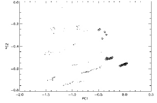
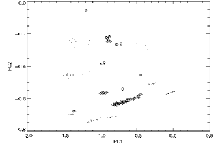
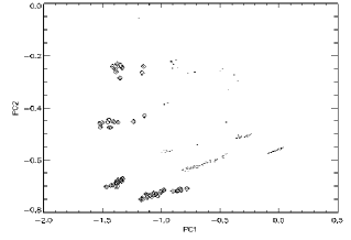
Figure 2: PC1-PC2 diagrams. In all diagrams, dots represent the results for all calculated models. Squares represent disks with radius 50 AU (upper left panel), 100 AU (upper right) and 150 AU (bottom).