Structuring and support by Alfvén waves around prestellar cores

Observations of molecular clouds show the existence of starless, dense cores, threaded by magnetic fields. Observed line widths indicate these dense condensates to be embedded in a supersonically turbulent environment. Under these conditions, the generation of magnetic waves is inevitable. In this paper, we study the structure and support of a 1D plane-parallel, self-gravitating slab, as a monochromatic, circularly polarized Alfvén wave is injected in its central plane. Dimensional analysis shows that the solution must depend on three dimensionless parameters. To study the nonlinear, turbulent evolution of such a slab, we use 1D high resolution numerical simulations. For a parameter range inspired by molecular cloud observations, we find the following. 1) A single source of energy injection is sufficient to force persistent supersonic turbulence over several hydrostatic scale heights. 2) The time averaged spatial extension of the slab is comparable to the extension of the stationary, analytical WKB solution. Deviations, as well as the density substructure of the slab, depend on the wave-length of the injected wave. 3) Energy losses are dominated by loss of Poynting-flux and increase with increasing plasma beta. 4) Good spatial resolution is mandatory, making similar simulations in 3D currently prohibitively expensive.

1 Introduction

Magnetic fields are observed in at least some molecular clouds (Crutcher 1999; Bourke et al. 2001). Whether all molecular clouds are threaded by magnetic fields is still under debate. Ward-Thompson et al. (2000) observe ordered magnetic fields on small scales of about 0.05 pc in, adopting their terminology, prestellar cores ($N\approx 10^{5}$ cm^-3). Also on somewhat larger scales, in star forming regions, ordered magnetic fields are reported (Matthews & Wilson 2002; Matthews et al. 2002). Coherent velocities in prestellar cores are observed on scales of about 0.01 pc (Barranco & Goodman 1998). On larger scales, observed line widths indicate supersonic motions. Taken together, these observations suggest dense condensates, threaded by magnetic fields, to be embedded in a supersonically turbulent environment. The generation of magnetic waves under such conditions is inevitable.

On larger scales, such magnetic waves are likely to be strongly damped (e.g. by ion-neutral friction or instabilities) or dominated by other processes (e.g. ISM-turbulence or incoming magnetic waves as studied by Elmegreen (1999)). This finding is in agreement with molecular cloud theories and observations. While some years ago it was thought that molecular clouds had to be supported against their self-gravity for at least $10^{8}$ years, new results are much more in agreement with a picture in which molecular clouds form, stars are born, and the clouds are dispersed, all within some $10^{6}$ years. Observations of molecular clouds in the solar neighborhood show that most clouds do form stars (Hartmann et al. 2001), from which it is concluded that star formation begins essentially as soon as a molecular cloud forms. Using stellar evolutionary tracks leads to the further conclusion that star formation in a molecular cloud takes place rapidly, once it has started (Palla & Stahler 2000). For stellar populations with an average age larger than about 3 Myr, no more molecular material can be detected (Hartmann et al. 2001, and references therein), indicating that star formation also ceases rapidly. Numerical simulations also support such a dynamical scenario (Ballesteros-Paredes et al. 1999; Elmegreen 2000; Mac Low 2002).

For smaller spatial scales, on the other hand, recent observations and simulations support the idea that magnetic fields and waves play an important role in the structuring of the environment of – possibly only transient – high density molecular clumps and the inhibition of accretion onto such clumps. Observations of the starless dense core L1512 and its immediate vicinity by Falgarone et al. (2001) show six dense filaments pointing towards the core and extending up to about 1 pc. The matter within each filament is observed to move towards the core while probably describing circular motions in the direction transverse to the filament. This motion and the orientation of the filaments make it likely that they are not merely part of the turbulent cascade within the cloud.

Heitsch et al. (2001) performed grid studies for 3D hydrodynamical and MHD simulations of the formation of persistent cores. They find that increasing spatial resolution leads to increased accretion in the hydrodynamical case, but to a decreased one in the MHD case. The authors ascribe this difference to better resolution of MHD waves, which then counteract accretion. For the case of a plane-parallel slab, at the boundary of which a monochromatic Alfvén wave is injected, 2D simulations with constant gravity by Pruneti & Velli (1997), as well as 2D and 3D simulations without gravity by Del Zanna et al. (2001), show the development of high-density filaments parallel to the direction of propagation of the Alfvén wave. Note that filamentation is observed only when open, not periodic, boundaries are used at the planes perpendicular to the direction of wave-propagation. Cho et al. (2002) have shown that magnetic fields can have rich structures well below the viscous dissipation scale, possibly affecting the density structure as well.

In this paper, we study the effect of magnetic waves in the framework of a simplified model, a 1D plane-parallel, self-gravitating slab with one central source of monochromatic, circularly polarized Alfvén waves. Related models have been investigated by other authors before (Gammie & Ostriker 1996; Martin et al. 1997; Fukuda & Hanawa 1999; Falle & Hartquist 2002; Kudoh & Basu 2003). The work here differs from previous 1D simulations in that we focus on the highly nonlinear, long-term evolution. Also, we consider only one central source of Alfvén waves, instead of injecting energy at each grid point, and we use open boundaries, not periodic ones. For this setting, we present a dimensional analysis as well as a parameter study based on numerical simulations.

Our results show that already one source of waves is sufficient to structure and support a turbulent slab in a quasi-static manner. The WKB solution for an Alfvén-wave supported, self-gravitating 1D slab by Martin et al. (1997) gives a good order of magnitude estimate for the average spatial extent of the turbulent slab, but fails to account for the rich interior structure. And while the Poynting-flux is constant in the WKB solution, there is substantial loss of Poynting-flux in the solution of the full equations. As governing parameters for deviations of the numerical solution from the analytical WKB solution we identify the initial, central Alfvén wave-length and the initial, central plasma beta. This is remarkable in view of the highly nonlinear, turbulent nature of the slab, where, for example, the true central Alfvén wave-length loses, even on average, any connection with its initial value after a fraction of a free-fall time. To observe both the structuring and support of the slab by magnetic waves, we find a good spatial resolution and high order of integration to be decisive.

The paper is organized as follows. In Sect. 2 we describe our physical model and the numerical method we use. We give a dimensional analysis of the problem in Sect. 3 before proceeding to the numerical results in Sect. 4. A discussion of our results follows in Sect. 5, conclusions are given in Sect. 6.

2 The model

2.1 Physical model problem

We consider a 1D (x-direction), plane-parallel, self-gravitating slab which we assume to be symmetric with respect to a central plane at $x=0$ (yz-plane, infinitely extended), where an Alfvén-wave is injected. In this geometry, all variables are functions of distance $x$ to the central plane and time $t$ only. Velocities and magnetic fields perpendicular to the x-direction are allowed, but gradients can occur only in the x-direction. To describe the time evolution of this slab, we use the ideal, isothermal MHD equations, including a source term to account for self-gravity. In their conservative formulation, these equations read:

$$\frac{\partial\rho}{\partial t}+\nabla\cdot(\rho\@vec{v}) = 0,$$ (1)

$$\frac{\partial(\rho\@vec{v})}{\partial t}+\nabla\cdot\left[\rho\@vec{v}\@vec{v}+p_{\mathrm{tot}}\@vec{I}-\frac{\@vec{B}\@vec{B}}{\mu_{\mathrm{0}}}\right] = \rho\@vec{g},$$ (2)

$$\frac{\partial\@vec{B}}{\partial t}+\nabla\cdot(\@vec{v}\@vec{B}-\@vec{B}\@vec{v}) = 0.$$ (3)

Here, $\rho$ denotes the mass density, $\@vec{v}=(v_{\mathrm{x}},v_{\mathrm{y}},v_{\mathrm{z}})$ the velocity, and $\@vec{B}=(B_{\mathrm{x}},B_{\mathrm{y}},B_{\mathrm{z}})$ the magnetic field. We will often use the notation $B_{\mathrm{\parallel}}$ for the constant background magnetic field $B_{\mathrm{x}}$, as well as $B_{\mathrm{\perp}}$ for the magnitude of the transverse magnetic field, and $B_{\mathrm{\perp 0}}$ for $B_{\mathrm{\perp}}$ at $x=0$ and $t=0$. Generally, a subscript $0$ to a variable refers to the initial ($t=0$) and, if space dependent, central ($x=0$) value of a variable. $\mu_{\mathrm{0}}$ is the magnetic permeability of free space, and $\@vec{I}$ is the identity tensor. $p_{\mathrm{tot}}=p_{\mathrm{th}}+(1/2\mu_{\mathrm{0}})\@vec{B}^{2}$ denotes the total pressure, where the thermal pressure is given by the isothermal equation of state $p_{\mathrm{th}}=\rho c_{\mathrm{s}}^{2}$, with $c_{\mathrm{s}}=\sqrt{RT}$ the isothermal sound speed. $T$ is the temperature of the gas and $R$ is the gas constant. Within the framework of our 1D model, the force exerted by self-gravity in the x-direction is given by $\@vec{g}=(g(x,t),0,0)$ with

$$g(x,t)=-4\pi G\int_{0}^{x}\rho(x^{\prime},t)dx^{\prime}.$$ (4)

$G$ denotes the gravitational constant. We consider only one sort of particle and consequently have no wave damping due to ion-neutral friction in our model. The average mass per particle is the mass $m_{\mathrm{H}}$ of a hydrogen atom.

For special cases, analytical solutions exist. For an infinitely extended slab with $\@vec{B}=\@vec{0}$, the stationary solution of the above model problem is given by the hydrostatic density distribution (Spitzer 1968),

$$\rho(x)=\rho_{\mathrm{0}}\cdot\frac{1}{\cosh^{2}(x/H)},$$ (5)

where $\rho_{\mathrm{0}}$ is the mass density at the central plane of the slab, $H=c_{\mathrm{s}}^{2}/(2\pi G{\cal M}^{\mathrm{hs}})$ is the hydrostatic scale height, and ${\cal M}^{\mathrm{hs}}=\int_{0}^{\infty}\rho(x)dx$ is the column density of the hydrostatic slab. $\rho_{\mathrm{0}}$ and $c_{\mathrm{s}}$ are free parameters of the solution.

For the case where the magnetic background field $B_{\mathrm{\parallel}}\neq 0$, and when a monochromatic, circularly polarized Alfvén wave is injected at the central plan of the slab, Martin et al. (1997) derived a stationary, analytical solution of the above model problem in the framework of a WKB approximation. In contrast to the hydrostatic solution, the WKB solution has three free parameters: $\rho_{\mathrm{0}}$, $c_{\mathrm{s}}$, and $B_{\mathrm{\perp}}$.

2.2 Model parameters and naming conventions

The full model problem as formulated in Sect. 2.1 has five free parameters. They could be specified in a dimensionless form, as we are going to discuss in Sect. 3. Guided by observations of molecular clouds, we choose, however, the following set of dimensional parameters: the background magnetic field $B_{\mathrm{\parallel}}$, the temperature $T$ of the slab, the initial, central mass density $\rho_{\mathrm{0}}$, the amplitude of the Alfvén wave, specified by either $B_{\mathrm{\perp}0}$ or $v_{\mathrm{\perp}0}=B_{\mathrm{\perp}0}/\sqrt{\mu_{\mathrm{0}}\rho_{\mathrm{0}}}$, and the frequency $\omega$ of the wave.

We varied parameters within limits that correspond roughly to observed parameters in molecular clouds: magnetic fields of 10-100 $\mu$G, temperatures between 5 K and 40 K, and central particle densities ranging from 250 to 2000cm^-3. For the wave frequency $\omega$ we have assumed values in the range $10^{4}\mbox{yr}\leq 2\pi/\omega\leq 2.5\cdot 10^{5}\mbox{yr}$. With this choice of parameters we are in a low-beta regime, the initial, central plasma beta $\beta_{0}=2c_{\mathrm{s}}^{2}/c_{\mathrm{A0}}^{2}$ lying in a range between 0.003 and 0.7. Here, $c_{\mathrm{A0}}=B_{\mathrm{\parallel}}/\sqrt{\mu_{\mathrm{0}}\rho_{\mathrm{0}}}$ denotes the initial, central Alfvén-speed. The corresponding Alfvén wave-length $\lambda_{\mathrm{A0}}=c_{\mathrm{A0}}\cdot 2\pi/\omega$, lies in a range between about 0.07 pc and 0.35 pc. The magnetic field $B_{\mathrm{\perp}0}$ corresponds to transverse velocities $v_{\mathrm{\perp}0}$ in the range between $2.5\cdot 10^{4}$cm/s and $3.2\cdot 10^{5}$cm/s. The detailed parameters for each of the performed simulations are given in Table 1 of the appendix. They are also reflected in the name of each simulation. For example, R20.10.25.4.40 is the simulation with $B_{\mathrm{\parallel}}=20\mu$G, $B_{\mathrm{\perp}}=10\mu$G, $2\pi/\omega=25\times 10^{4}$ years, a central density of $N_{\mathrm{0}}=4\times 250$ particles per cm³, and $T=40$K.

2.3 Numerical solution

2.3.1 Numerical method

In our simulations, we consider a slab of finite (not infinite) spatial extension ${\cal D}$. We use a finite volume method on an equidistant spatial grid to solve the ideal, isothermal MHD equations, Eqs. 1–3. Fluxes are computed using a second order in time and third order in space stabilized Lax-Friedrichs solver as described in Barmin et al. (1996). As is shown in Barmin et al. (1996), the accuracy of this solver is comparable to that of a second order Riemann solver. Self-gravity is taken into account using a Strang-splitting (Strang 1968).

2.3.2 Initial conditions

At time $t=0$ we assume the slab to have a density distribution according to the analytical WKB solution of Martin et al. (1997) for a given set of parameters as specified in Table 1. The velocity in the x-direction, as well as the transverse components of the velocity and the magnetic field, we set to zero. The magnetic field in x-direction, $B_{\mathrm{\parallel}}$, and the temperature $T$, we set to the values given in Table 1. The mass column density of the initial WKB solution, within the computational domain and to infinity, we denote by ${\cal M}_{\mathrm{0}}$ and ${\cal M}_{\mathrm{0}}^{\mathrm{\infty}}$ respectively.

2.3.3 Boundary conditions

Boundary conditions are implemented using four boundary cells at each of the two domain boundaries. Note that in this way we merely control the physical variables set in these cells. The fluxes entering and leaving the domain are determined by the interaction of the solution as set in the boundary cells and the numerical solution within the computational domain.

In the boundary cells at the inner domain boundary $(x=0)$, the physical variables are set in accordance with a left-handed, circularly polarized Alfvén-wave, whose velocity amplitude $v_{\mathrm{\perp}}$ we keep fixed in time, $v_{\mathrm{\perp}}=v_{\mathrm{\perp 0}}$. Allowing $v_{\mathrm{x}}$ and $\rho_{\mathrm{0}}$, and thus $B_{\mathrm{\perp}}$, to vary according to the solution in the domain, this yields:

$$\rho(x) = \rho(-x),$$

$$v_{\mathrm{x}}(x) = -v_{\mathrm{x}}(-x),$$

$$v_{\mathrm{y}}(x) = v_{\mathrm{\perp}}\cos(\omega(t-\Delta t)),$$

$$v_{\mathrm{z}}(x) = v_{\mathrm{\perp}}\sin(\omega(t-\Delta t)),$$

$$B_{\mathrm{x}}(x) = B_{\mathrm{\parallel}},$$

$$B_{\mathrm{y}}(x) = v_{\mathrm{y}}(x)\cdot\sqrt{\mu_{\mathrm{0}}\rho(x)},$$

$$B_{\mathrm{z}}(x) = v_{\mathrm{z}}(x)\cdot\sqrt{\mu_{\mathrm{0}}\rho(x)}.$$ (6)

For the calculation of the time retardation $\Delta t=x/c_{\mathrm{A}}$ we take into account that $c_{\mathrm{A}}$ varies with $x$ and $t$.

At the outer boundary, we distinguish two cases. If $v_{x}({\cal D},t)>0$ we use a zeroth order extrapolation for all conserved variables. If $v_{x}({\cal D},t)<0$ we use a zeroth order extrapolation for $\@vec{v}$ and $\@vec{B}$, but restrict the density to $10^{-4}\rho_{\mathrm{0}}$. Note that these outer boundary conditions allow for both accretion or loss of matter, energy, and momentum. Associated changes in the mass column density over the domain, ${\cal M}(t)$, are, however, mostly less than 2% (see Table 1).

We have chosen open boundaries as these match best with our intention to investigate the effect of only one source of Alfvén waves. Using periodic boundary conditions instead would implicitly introduce several sources of Alfvén waves, separated from each other by a distance $2{\cal D}$.

2.3.4 Choice of domain size, discretization, and integration time

For the simulations we chose a domain of size ${\cal D}=6$ pc, or about 20 hydrostatical scale heights, covered by 5000 cells. With this choice, we fulfill the following four basic requirements. 1) The initial WKB solution fits well on the domain, 90% of its column density ${\cal M}_{\mathrm{0}}$ occupy less than 60% of the domain. 2) The numerical solution fits well on the domain, 90% of its column density ${\cal M}(t)$ are contained in the inner half of the domain and ${\cal M}(t)$ barely changes with time. 3) The hydrostatic solution is covered by sufficiently many cells. 4) The numerical solution does not depend on the discretization. Several grid studies show 5000 cells to be both necessary and sufficient (see Sect. 5.4 and Fig. 8). We followed all our simulations for $2\cdot 10^{7}$ years, or about 20 sound crossing times of the hydrostatic scale height.

3 Dimensional analysis

Before coming to the numerical results in Sect. 4, we present a dimensional analysis of the model problem formulated in Sect. 2.1. Dimensional parameters which completely specify the problem are the initial mass column density ${\cal M}_{\mathrm{0}}^{\mathrm{\infty}}$, the magnetic field $B_{\mathrm{\parallel}}$, the sound speed $c_{\mathrm{s}}$, the wave frequency $\omega$ of the imposed oscillations, and their velocity amplitude $v_{\mathrm{\perp}0}$ at the central plane. Since Alfvén wave propagation and self-gravity are essential parts of the problem, the dimensional constants $\mu_{\mathrm{0}}$ and $G$ also determine the solution. The solution in infinite space is determined by these seven dimensional input parameters. For our finite computational domain this is no longer strictly true, but we shall neglect this complication for the moment.

From the seven dimensional input parameters we can build four natural reference values for length, time, mass density, and magnetic field. The three extra dimensional parameters would then be associated with three dimensionless quantities that can be constructed from the seven parameters. In infinite space, the (suitably normalized) physical quantities in the solution would be functions of the normalized time and space variables and of these three dimensionless input parameters.

3.1 Natural dimensional reference values

The four natural dimensional reference values (subscript $\mathrm{u}$ for ’unity’ in the following) should be defined such that none of them would approach zero or infinity when some parameters of the problem take expectedly large or small values. For example, we should allow $\omega$ to become very large, as it might be in the WKB limit and as it is possibly met in actual situations. Similarly, $c_{\mathrm{s}}$ may, in some clouds, become small enough to be neglected. This means that sensible natural references should be constructed from ${\cal M}_{\mathrm{0}}^{\mathrm{\infty}}$, $B_{\mathrm{\parallel}}$, $v_{\mathrm{\perp}0}$, $\mu_{\mathrm{0}}$ and $G$ alone. Obviously $B_{\mathrm{\parallel}}$ provides a reference magnetic field, $B_{\mathrm{u}}$, while the references of mass density, length, and time, $\rho_{\mathrm{u}}$, $d_{\mathrm{u}}$ and $t_{\mathrm{u}}$, can be defined from ${\cal M}_{\mathrm{0}}$, $v_{\mathrm{\perp}0}$ and $G$ alone. Straightforward dimensional analysis shows that these four reference scales can be taken as:

$$B_{\mathrm{u}} = B_{\mathrm{\parallel}},$$

$$\rho_{\mathrm{u}} = \frac{2\pi G({\cal M}_{\mathrm{0}}^{\mathrm{\infty}})^{2}}{v_{\mathrm{\perp}0}^{2}},$$

$$d_{\mathrm{u}} = \frac{v_{\mathrm{\perp}0}^{2}}{2\pi G{\cal M}_{\mathrm{0}}^{\mathrm{\infty}}},$$

$$t_{\mathrm{u}} = \frac{v_{\mathrm{\perp}0}}{2\pi G{\cal M}_{\mathrm{0}}^{\mathrm{\infty}}}.$$ (7)

The factors $2\pi$ were inserted for convenience, such that $\rho_{\mathrm{u}}$ and $d_{\mathrm{u}}$ are the central density and scale height of a self-gravitating isothermal sheet with sound speed $v_{\mathrm{\perp}}$ that would have, in infinite space, a column density ${\cal M}_{\mathrm{0}}^{\mathrm{\infty}}$. The reference time $t_{\mathrm{u}}=d_{\mathrm{u}}/v_{\mathrm{\perp}0}$ is of the order of the Jeans period associated with $\rho_{\mathrm{u}}$.

From the three remaining dimensional input parameters $\mu_{\mathrm{0}}$, $c_{\mathrm{s}}$ and $\omega$ we can form, given these references, 3 natural dimensionless numbers, for example:

$$\alpha_{\mathrm{u}} = \frac{v_{\mathrm{\perp}0}^{2}}{\left(B_{\mathrm{u}}^{2}/(\mu_{\mathrm{0}}\rho_{\mathrm{u}})\right)},$$

$$\beta_{\mathrm{u}} = \frac{2c_{S}^{2}}{\left(B_{\mathrm{u}}^{2}/(\mu_{\mathrm{0}}\rho_{\mathrm{u}})\right)},$$

$$W_{\mathrm{u}} = \frac{\omega}{\sqrt{2\pi G\rho_{\mathrm{u}}}}.$$ (8)

The parameter $\alpha_{\mathrm{u}}$ compares the imposed velocity amplitude $v_{\mathrm{\perp}0}$ to the reference Alfvén velocity $c_{\mathrm{Au}}$, defined by $c_{\mathrm{Au}}^{2}=B_{\mathrm{u}}^{2}/(\mu_{\mathrm{0}}\rho_{\mathrm{u}})$. The parameter $\beta_{\mathrm{u}}$ is the ratio of the reference gas pressure to the magnetic pressure of $B_{\mathrm{u}}$. The parameter $W_{\mathrm{u}}$ is a WKB parameter. Clearly, neither the set of the four reference dimensional values nor the set of the three input dimensionless numbers is uniquely defined. Other dimensional reference values could be obtained by multiplying the chosen ones by any function of the dimensionless input numbers $\alpha_{\mathrm{u}}$, $\beta_{\mathrm{u}}$, and $W_{\mathrm{u}}$. Similarly, the above set of three such numbers could be replaced by three other arbitrary functions of them.

3.2 Dimensional reference values from WKB solution

The reference quantities defined in Eq. 7 need not be very close to the actual values of the physical quantities in the solution, even near the central plane. It may be felt desirable, however, that the reference values be as close as possible to actual ones, even at the price of defining the reference values in a more sophisticated way than $\rho_{\mathrm{u}}$, $d_{\mathrm{u}}$ and $t_{\mathrm{u}}$. If the WKB solution is to be a guide, such estimates could be obtained from the solution of Martin et al. (1997). From this solution, it is possible to relate the central density $\rho_{\mathrm{0}}$ of a solution to its column density ${\cal M}_{\mathrm{0}}$ in the finite computational domain of thickness ${\cal D}$ and to the total column density to infinity, ${\cal M}_{0}^{\mathrm{\infty}}$. The limited extent of the computational domain is reflected in the fact that the ratio $({\cal M}_{\mathrm{0}}/{\cal M}_{\mathrm{0}}^{\mathrm{\infty}})$ is less than unity. A scale length $d^{\mathrm{wkb}}_{\mathrm{0}}$ may then be defined as the distance from the central plane of the slab where 90% of the column density ${\cal M}_{\mathrm{0}}$ are reached. The time scale $t_{\mathrm{0}}$ can be defined as $t_{\mathrm{0}}=(2\pi G\rho_{\mathrm{0}})^{-1/2}$. The reference value of the magnetic field may be chosen as before, $B_{\mathrm{0}}=B_{\mathrm{\parallel}}$.

In analogy with Eq. 8, dimensionless numbers $\alpha_{\mathrm{0}}$, $\beta_{\mathrm{0}}$, and $W_{\mathrm{0}}$ can be introduced. Note that $\beta_{\mathrm{0}}$ is, in fact, identical to $\beta_{\mathrm{0}}$ as given in Sect. 2.2. An Alfvén-velocity can be defined by $c_{\mathrm{A0}}^{2}=B_{\mathrm{\parallel}}^{2}/(\mu_{\mathrm{0}}\rho_{\mathrm{0}})$, and Alfvén wave-length by $\lambda_{\mathrm{A0}}=2\pi c_{\mathrm{A0}}/\omega$.

Aliases to the WKB parameter $W_{\mathrm{0}}$ could be used as well. In particular, one could prefer the ratio of the WKB length scale to the Alfvén wavelength associated with $B{\mathrm{\parallel}}$ and $\rho_{\mathrm{0}}$, $W_{\mathrm{\lambda A0}}=\lambda_{\mathrm{A0}}/d^{\mathrm{wkb}}_{\mathrm{0}}$. For our simulations, the values for a number of these dimensionless parameters are listed in Table 1.

3.3 Reference values for substructure scale

Unlike the WKB solution, the numerical solution of the model problem from Sect. 2.1 is far from smooth (see e.g. Fig. 3). And while the lengths $d_{\mathrm{u}}$ or $d^{\mathrm{wkb}}_{\mathrm{0}}$ are natural estimates for the global size of the mass distribution, the natural scale length associated with substructures induced by the wave is, of course, quite different. It is either of the order of the reference Alfvén wavelength $\lambda_{\mathrm{Au}}=2\pi c_{\mathrm{Au}}/\omega$ or of the Alfvén wavelength associated with the WKB reference quantities, $\lambda_{\mathrm{A0}}=2\pi c_{\mathrm{A0}}/\omega$. These two scales are of the same order of magnitude for a wave-supported cloud. The actual characteristic scale of cloud substructure is the product of any one of them with a function of the dimensionless input parameters. On physical grounds, we expect, however, this function to be of the order of unity, since no other small length scale is likely to play an important role. In the low-$\beta$ regime we consider, the sonic wavelength $2\pi c_{S}/\omega$ is usually much shorter and sound perturbations nonlinearly evolve into shocks anyway, so that this sonic wavelength is not expected to show up in the spectrum of the fluctuations, except perhaps at the level of the very small thickness of the dense sheets that form.

In the next section, we present the numerical solutions for the model problem from Sect. 2.1 for various parameter sets. Note that our study, inspired by molecular clouds, covers only a small part of the entire parameter space. For this part of the parameter space, we identify and discuss some of the dependences indicated by the dimensional analysis.

4 Numerical results

The injection of magnetic waves at the central plane of the self-gravitating slab has two major consequences: the slab becomes supersonically turbulent and its spatial extension is clearly larger than in hydrostatic equilibrium.

Neither of these consequences is surprising. The energy provided by the injected wave must result in additional support of the slab against its self-gravity. Density inhomogeneities are to be expected since within the frame of linear analysis a parametric instability of the injected Alfvén wave exists (Derby 1978; Goldstein 1978; Turkmani & Torkelsson 2003). Early on in our simulations we observe the associated growth of high density sheets, which is accompanied by the destruction of the transverse magnetic field (see Fig. 1). Note also that Malara & Velli (1996) and Malara et al. (2000) demonstrated that even a non-monochromatic spectrum of Alfvén waves is subject to parametric instability with linear and nonlinear growth rates of the same order of magnitude as in the monochromatic case.

So far the turbulent, nonlinear evolution of such a system is, however, not well investigated. The results we present in the following demonstrate that the same parameters which govern the parametric instability, $\lambda_{\mathrm{A0}}$ and $\beta_{\mathrm{0}}$, are also of crucial importance for the nonlinear, turbulent solution. This despite the fact that the true, time averaged values of these quantities at $x=0$ (and close by) deviate substantially from $\lambda_{\mathrm{A0}}$ and $\beta_{\mathrm{0}}$.

Figure 1: Early on in all our simulations, high density sheets develop under the influence of the parametric instability of the Alfvén-wave, while the transverse magnetic field is partly destroyed. The figure is a snapshot of simulation R20.20.5.4.10 after $2.1\cdot 10^{5}$ years. Shown are the density (solid line) and the energy density of the transverse magnetic field (dashed line), normalized to their initial, central values, as functions of distance to the central plane (x-axis, in units of $\langle d^{\mathrm{sol}}\rangle_{\mathrm{t}}$, the time averaged slab extension). The dotted curves denote $N/N_{\mathrm{0}}$ (lower curve) and $E^{\mathrm{\perp}}_{\mathrm{mag}}/E^{\mathrm{\perp}}_{\mathrm{mag0}}$ (upper curve) of the initial WKB solution.

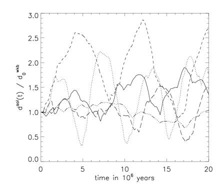
Figure 2: a) The ratio of $\lambda_{\mathrm{A0}}$ to the extension of the WKB solution determines how well $\langle d^{\mathrm{sol}}\rangle_{\mathrm{t}}$ and $d^{\mathrm{wkb}}_{\mathrm{0}}$ agree. Shown is $\langle d^{\mathrm{sol}}\rangle_{\mathrm{t}}/d_{\mathrm{0}}^{\mathrm{wkb}}$ as a function of $\lambda_{\mathrm{A0}}/d_{\mathrm{0}}^{\mathrm{wkb}}$ for the different runs. The dotted line is the corresponding linear least square fit. b) The spatial extension of the nonlinear solution is more or less time variable and can show distinct oscillations. For details on the oscillation period, see text. Shown is $d^{\mathrm{sol}}(t)/d^{\mathrm{wkb}}_{\mathrm{0}}$ as a functions of time (x-axis, in million years) for three oscillatory runs R20.20.25.4.10 (solid), R100.10.5.4.10 (dashed), and R100.45.5.8.10 (dotted), as well as for two runs without a clear oscillation, R20.10.12.1.10 (dash-three-dots) and R100.45.5.4.10 (long dashes).

4.1 Spatial extension of turbulent slab

We find that the time averaged spatial extension of the solution roughly agrees with the spatial extension of the corresponding WKB solution. As a function of time, the spatial extension $d^{\mathrm{sol}}(t)$ can oscillate but does not have to. $d^{\mathrm{sol}}(t)$ we define in analogy with $d_{\mathrm{0}}^{\mathrm{wkb}}$ (see Sect. 3) as the distance where the column density reaches 90% of ${\cal M}(t)$. We similarly define the extension $d^{\mathrm{hs}}(t)$ and $d^{\mathrm{wkb}}(t)$ of the corresponding hydrostatical and WKB solutions, where corresponding means that at time $t$ the three solutions have the same ${\cal M}(t)$. Finally, we denote by $\left<.\right>_{\mathrm{t}}$ the time average between $5\cdot 10^{6}$ and $2\cdot 10^{7}$ years.

4.1.1 Dependence on system parameters

In all our simulations, the time averaged extension $\langle d^{\mathrm{sol}}\rangle_{\mathrm{t}}$ of the slab agrees to within a factor of three with the spatial extension of the WKB solution $d^{\mathrm{wkb}}_{\mathrm{0}}$. The dominant parameters governing the extension of the slab are, therefore, the parameters governing the WKB solution, i.e. $\rho_{0}$, $B_{\mathrm{\perp}}$, and $T$.

Deviations from the spatial extension of the WKB solution we find to depend linearly on the dimensionless WKB parameter $W_{\mathrm{\lambda A0}}=\lambda_{\mathrm{A0}}/d^{\mathrm{wkb}}_{\mathrm{0}}$. Fig. 2a shows the ratio of the spatial extensions $\langle d^{\mathrm{sol}}\rangle_{\mathrm{t}}/d^{\mathrm{wkb}}_{\mathrm{0}}$ as a function of $\lambda_{\mathrm{A0}}/d^{\mathrm{wkb}}_{\mathrm{0}}$ for the different runs. A linear least square fit, also shown in the figure, gives a dependence $\langle d^{\mathrm{sol}}\rangle_{\mathrm{t}}=\alpha\lambda_{\mathrm{A0}}+\beta d^{\mathrm{wkb}}_{\mathrm{0}}$ with $\alpha=4.06$ and $\beta=0.36$. Linear fits of similar quality are obtained if instead of $d^{\mathrm{wkb}}_{\mathrm{0}}$ one uses as scaling parameter $\langle d^{\mathrm{hs}}\rangle_{\mathrm{t}}$, or $\langle d^{\mathrm{wkb}}\rangle_{\mathrm{t}}$. For the last case, the fitting parameters are $\alpha=3.86$ and $\beta=0.37$. If instead of $\lambda_{\mathrm{A0}}$ we consider the time average of the true Alfvén wave-length $\langle\lambda_{\mathrm{A}}\rangle_{\mathrm{t}}$ at or close to the slab center, we cannot identify any such clear dependence. $\langle\lambda_{\mathrm{A}}\rangle_{\mathrm{t}}$ is usually larger than $\lambda_{\mathrm{A0}}$ by a factor of about 2 to 8.

From Fig. 2a it can be seen that best agreement between $\langle d^{\mathrm{sol}}\rangle_{\mathrm{t}}$ and $d^{\mathrm{wkb}}_{\mathrm{0}}$ is obtained around $\lambda_{\mathrm{A0}}/d^{\mathrm{wkb}}_{\mathrm{0}}=0.17$. The deviations at larger values of $\lambda_{\mathrm{A0}}/d^{\mathrm{wkb}}_{\mathrm{0}}$ are not too surprising. A basic assumption for the validity of WKB theory is that the density changes only on scales much larger than the Alfvén wave-length. This assumption fails to hold as $\lambda_{\mathrm{A0}}/d^{\mathrm{wkb}}_{\mathrm{0}}$ increases. For the deviations at small values of $\lambda_{\mathrm{A0}}/d^{\mathrm{wkb}}_{\mathrm{0}}$ we have checked that they are not caused by a too coarse spatial discretization, which would cause artificial wave-damping and thus reduced support against self-gravity. Increasing the spatial resolution by a factor of four left the nonlinear solution unchanged. Instead, the true reason again lies in the failure of the WKB approach to be valid. The mass distribution in the system still consists of thin, dense sheets separated by more diffuse medium. As the sheet thickness is much less than the Alfvén wavelength in the tenuous medium, the conditions for a WKB description are not met. We come back to this point in more detail in Sect. 5.1.

Besides the dominant effect of $\lambda_{\mathrm{A0}}/d^{\mathrm{wkb}}_{\mathrm{0}}$, Fig. 2a suggests $\beta_{\mathrm{0}}$ to have a second order effect. Simulations with identical ratio $\lambda_{\mathrm{A0}}/d^{\mathrm{wkb}}_{\mathrm{0}}$ usually have a larger extension for smaller $\beta_{\mathrm{0}}$.

In view of what was said in Sect. 3, the average slab thickness must equal the reference scale $d_{\mathrm{0}}^{\mathrm{wkb}}$ multiplied by a function of $\alpha_{\mathrm{0}}$, $\beta_{\mathrm{0}}$ and $W_{\mathrm{\lambda A0}}$. In the limit of very small pressure the dependence on $\beta_{\mathrm{0}}$ disappears. In the limit of very large $W_{\mathrm{\lambda A0}}$, that is very small $\lambda_{\mathrm{A0}}/d^{\mathrm{wkb}}_{\mathrm{0}}$, the dependence on $W_{\mathrm{\lambda A0}}$ also disappears. There may remain some dependence on $\alpha_{\mathrm{0}}$, which Fig. 2a indicates to be weak. The ratio $\langle d^{\mathrm{sol}}\rangle_{\mathrm{t}}/d^{\mathrm{wkb}}_{\mathrm{0}}$ then approaches a value which is apparently close to $(1/2)$. For higher values of $\lambda_{\mathrm{A0}}/d^{\mathrm{wkb}}_{\mathrm{0}}$, we expect some dependence of $\langle d^{\mathrm{sol}}\rangle_{\mathrm{t}}/d^{\mathrm{wkb}}_{\mathrm{0}}$ on this parameter, which may be represented by a Taylor expansion to first order for not too large $\lambda_{\mathrm{A0}}/d^{\mathrm{wkb}}_{\mathrm{0}}$. This is in rough agreement with what is seen in Fig. 2a, and is consistent with the idea that the larger the Alfvén wave-length, the larger the spacing between dense sheets, and the thicker the system.

Figure 3: For simulations with the same Alfvén wave-length $\lambda_{\mathrm{A0}}$ and temperature $T$, but otherwise widely different parameters, the size of the voids (black, $N=10^{-1}$ cm^-3) separating the high density sheets (white, $N=10^{4}$ cm^-3) is about the same. Comparison with Fig. 4 shows the effect of different values of $\lambda_{\mathrm{A0}}$ and $T$. The general density stratification leads to larger voids at larger distances. Shown is the logarithmic particle density as a function of space (x-axis, in units of 6 pc) and time (y-axis, in units of $10^{6}$ years) for runs a) R20.20.25.4.10 and d) R100.10.5.4.10.

4.1.2 Time variability of slab extension

As a function of time, the spatial extension $d^{\mathrm{sol}}(t)$ of the slab can be very variable but does not have to be. We mention already here that the substructure of the slab, voids and high density sheets, always shows oscillatory motions (see Sect. 4.2 and Fig. 3). In Fig. 2b, the ratio of $d^{\mathrm{sol}}(t)/d^{\mathrm{wkb}}_{\mathrm{0}}$ is shown as a function of time for five runs, representative of the total of our simulations. As can be seen, only some of the runs show a strong variability while others have a more or less constant extension. A measure for the strength of this time variability is the standard deviation $\sigma_{\mathrm{d}}$ of $d^{\mathrm{sol}}(t)/d^{\mathrm{wkb}}_{\mathrm{0}}$. Using for the calculation of $\sigma_{\mathrm{d}}$ the same time interval as for the time averages, we find the relative standard deviation $\sigma^{\mathrm{rel}}_{\mathrm{d}}=\sigma_{\mathrm{d}}/(\langle d^{\mathrm{sol}}\rangle_{\mathrm{t}}/d^{\mathrm{wkb}}_{\mathrm{0}})$ to lie in an interval of $0.1\;\hbox to0.0pt{\lower 2.5pt\hbox{$\sim$}\hss}\raise 1.5pt\hbox{$<$}\;\sigma^{\mathrm{rel}}_{\mathrm{d}}\;\hbox to0.0pt{\lower 2.5pt\hbox{$\sim$}\hss}\raise 1.5pt\hbox{$<$}\;0.9$ (see Table 1).

In about half of our simulations, the variability takes the form of a roughly periodic oscillation. The period of the oscillation is, however, not always well defined. Twice the sound crossing time of the average slab thickness, $T_{\mathrm{s}}=2\langle d^{\mathrm{sol}}\rangle_{\mathrm{t}}/c_{\mathrm{s}}$, is often close to the observed period $T_{\mathrm{obs}}$. The ratio $T_{\mathrm{obs}}/T_{\mathrm{s}}$ averages over the different runs to a value close to 0.95. However, this ratio, normalized to its average value, has significant scatter of the order of 0.8. Moreover, the fact that our slabs are more wave-supported than gas pressure supported makes it difficult to understand a scaling like $T_{\mathrm{obs}}\sim T_{\mathrm{s}}$ on physical grounds. A more natural scaling, as we will show in Sect. 5.2, would be that the oscillation period is proportional to twice the crossing time of the average slab thickness at velocity $v_{\mathrm{\perp 0}}$. For $T_{\mathrm{v\perp 0}}=2\langle d^{\mathrm{sol}}\rangle_{\mathrm{t}}/v_{\mathrm{\perp 0}}$ the ratio $T_{\mathrm{obs}}\sim T_{\mathrm{v\perp 0}}$ averages, over our different runs, to 3.4 with a scatter of 0.4. For $T_{\mathrm{v\perp 0}}=2d^{\mathrm{wkb}}_{\mathrm{0}}/v_{\mathrm{\perp 0}}$ the average is 3.6 with a scatter of only 0.2. Thus, to within a factor of order unity, but somewhat larger than unity, our simulations are also consistent with $T_{\mathrm{obs}}$ being proportional to $T_{\mathrm{v\perp 0}}$.

Figure 4: Smaller voids (black, $N=10^{-1}$ cm^-3) separating the high density sheets (white, $N=10^{4}$ cm^-3) are obtained for smaller $\lambda_{\mathrm{A0}}$ and / or higher temperatures $T$. a) Run R20.20.12.4.10 has the same temperature $T$ as run R20.20.25.4.10 in Fig. 3, but only half the value of $\lambda_{\mathrm{A0}}$. b) Run R20.20.25.4.40 has the same $\lambda_{\mathrm{A0}}$ as run R20.20.25.4.10 in Fig. 3 but a four times higher temperature $T$. Shown is the logarithmic particle density as a function of space (x-axis, in units of 6 pc) and time (y-axis, in units of $10^{6}$ years).

4.2 Inhomogeneous structure of turbulent slab

Under the influence of both the injected wave and self-gravity, the interior structure of the slab becomes very inhomogeneous, substructure develops. This substructure is the result of time-dependent, nonlinear effects and as such is beyond the reach of WKB theory. Again, we find $\lambda_{\mathrm{A0}}$ to play a critical role, but now the temperature of the slab has an effect as well.

The density distribution is characterized by extended, low density voids and narrow, high density sheets. In these low density voids, the other variables, $\@vec{v}$ and $\@vec{B}$, remain nearly constant. Therefore, the density substructure is a good mirror for their substructure as well, and we restrict ourselves to density in the following. To characterize the density substructure in our gravitationally stratified slab, we represent the time series of 1D density distributions as a 2D grey-scale plot. Low density regions then appear as more or less extended (dark) patches, while high density sheets take the form of thin (bright) lines.

Fig. 3 shows such a representation of the density for two runs. Apparent also in this representation is the presence (run R100.10.5.4.10) or absence (run R20.20.25.4.10) of a global oscillation of the slab. However, it can also be seen that, independent of the existence of a global oscillation, the high density sheets within the slab undergo oscillatory motions. The motion of a single sheet is roughly parabolic, but may be interrupted at any time as two sheets collide. Different sheets can have widely different oscillation periods, which are mostly much smaller than the period of the global oscillation of the slab.

This motion of the high density sheets, together with the number of sheets, determines the size of the voids (dark patches in Fig. 3) in the 2D representation of the data. We call this the scale of the substructure, a larger scale substructure thus referring to an overall large size of the voids. Based on the only qualitative measure of the grey-scale plots, we find that this scale of the substructure is, in essence, determined by $\lambda_{\mathrm{A0}}$ and temperature $T$. The size of the substructure in the two runs shown in Fig. 3, which have the same $\lambda_{\mathrm{A0}}$ and temperature $T$, but otherwise widely different parameters, is very similar. This becomes even more apparent if Fig. 3 is compared with Fig. 4, where simulations with only half the Alfvén wave-length (Fig. 4a) and four times the slab temperature $T$ (Fig. 4b) are shown. On the other hand, the scale of the density distribution for the two simulations shown in Fig. 4 is again similar. This suggest that augmenting the temperature by a factor of four has the same effect as reducing the Alfvén wave-length $\lambda_{\mathrm{A0}}$ by a factor of two. Or, put otherwise, that the scale of the density substructure in space and time depends on the ratio $\sqrt{T}/\lambda_{\mathrm{A0}}$ or, equivalently, on $\sqrt{\beta_{\mathrm{0}}}\omega$. We currently have, however, no quantitative measure to further corroborate this speculation.

The dominant role of $\lambda_{\mathrm{A0}}$ for the scale of the density distribution may have been anticipated from what was said towards the end of Sect. 3 as well as from parametric instability theory (Derby 1978; Goldstein 1978). Analytical results for the linear regime indeed show the separation of density disturbances to increase with increasing Alfvén wave-length. On the other hand, the system we consider is highly nonlinear and $\lambda_{\mathrm{A0}}$ soon loses its meaning even on average.

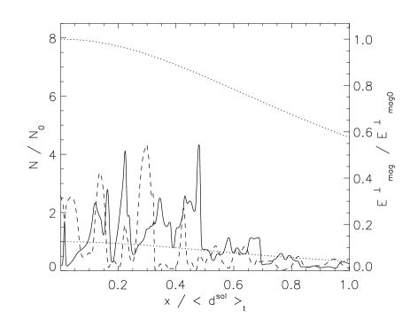
Figure 5: The energy $E^{\mathrm{\perp}}_{\mathrm{mag}}$ of the transverse magnetic field is very inhomogeneous. It is generally smaller than in the corresponding WKB solution and not correlated with the density substructure. Shown are the density (solid line) and the energy density of the transverse magnetic field (dashed line), normalized to their initial, central values, as functions of distance to the central plane (x-axis, in units $\langle d^{\mathrm{sol}}\rangle_{\mathrm{t}}$) at the example of simulation R20.20.5.4.10 at a time of $2.07\cdot 10^{7}$ years. The dotted curves denote $N/N_{\mathrm{0}}$ (lower curve) and $E^{\mathrm{\perp}}_{\mathrm{mag}}/E^{\mathrm{\perp}}_{\mathrm{mag0}}$ (upper curve) of the corresponding WKB solution.

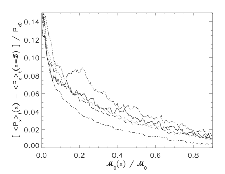
Figure 6: a) Change of time averaged Poynting-flux, between the central plane and $\langle d^{\mathrm{sol}}\rangle_{\mathrm{t}}$, in units of the corresponding WKB Poynting flux, $P_{\mathrm{x0}}$ as a function of $\sqrt{\beta_{\mathrm{0}}}$ for the different runs we have performed. b) Change of time averaged Poynting-flux, $\Delta\langle P^{\mathrm{sol}}_{\mathrm{x}}\rangle_{\mathrm{t}}$, in units of the corresponding WKB Poynting flux, as a function of increasing, relative column density ${\cal M}_{\mathrm{0}}(x)/{\cal M}_{\mathrm{0}}$ for five runs, all with $\beta_{\mathrm{0}}=0.087$: R20.20.5.4.10 (dash-dotted), R20.20.10.4.10 (long dashes), R20.20.12.4.10 (dotted), R20.20.17.4.10 (solid), R20.20.25.4.10 (dash-three-dots).

4.3 Energy of turbulent slab

At the central plane, we constantly feed energy into the slab. The energy provided by this ’one point forcing’ penetrates far into the slab, despite the gradual destruction through isothermal shocks and viscous dissipation. Note that the viscous dissipation is merely given by the numerical method and the discretization, and may not accurately mimic real viscosity, diffusion, or resistivity. The energy density of the transverse magnetic field is far from smooth and is generally smaller than its initial WKB value. A typical situation at later times is shown in Fig. 5. The density substructure leads to wave reflection and shock formation. Occasionally, the WKB value of $E^{\mathrm{\perp}}_{\mathrm{mag}}$ can be exceeded, as two high density sheets move against each other, thus compressing the transverse magnetic field between them.

4.3.1 Loss of Poynting-flux

Unlike in the WKB solution, the Poynting-flux in our numerical solution is neither constant in space nor time. Let us denote by $P_{\mathrm{x0}}$ the Poynting-flux of the initial WKB solution and by $\langle P_{\mathrm{x}}\rangle_{\mathrm{t}}$ the time averaged x-component of the true Poynting-flux. We find that the change $\Delta\langle P^{\mathrm{sol}}_{\mathrm{x}}\rangle_{\mathrm{t}}$ of the Poynting-flux over a distance $\langle d^{\mathrm{sol}}\rangle_{\mathrm{t}}$ from the central plan of the slab lies in a range $0.03\;\hbox to0.0pt{\lower 2.5pt\hbox{$\sim$}\hss}\raise 1.5pt\hbox{$<$}\;\Delta\langle P^{\mathrm{sol}}_{\mathrm{x}}\rangle_{\mathrm{t}}/P_{\mathrm{x0}}\;\hbox to0.0pt{\lower 2.5pt\hbox{$\sim$}\hss}\raise 1.5pt\hbox{$<$}\;0.4$. The ratio depends about linearly on $\sqrt{\beta_{\mathrm{0}}}$, as can be seen in Fig. 6a. In view of the results in Sect. 4.2, this dependence suggests a connection between the loss of Poynting-flux and the amount of density structure we have in the slab. There we have seen that larger values of $\sqrt{T}/\lambda_{\mathrm{A0}}$, which implies larger values of $\sqrt{\beta_{\mathrm{0}}}$, correlate with a finer scale density structure.

Largest losses of Poynting-flux occur in the innermost region of the slab, and more than 90% of the total loss of Poynting-flux over the entire computational domain occurs within a distance $\langle d^{\mathrm{sol}}\rangle_{\mathrm{t}}$ of the central plane of the slab. Fig. 6b shows the spatial variation of the loss of Poynting-flux. There, $\langle P_{\mathrm{x}}\rangle_{\mathrm{t}}(x)-\langle P_{\mathrm{x}}\rangle_{\mathrm{t}}(x={\cal D})$ is shown, in units of $P_{\mathrm{x0}}$, as a function of increasing, relative column density ${\cal M}_{\mathrm{0}}(x)/{\cal M}_{\mathrm{0}}$ for five runs. Except for the value of $\omega$, the runs have identical parameters with a value of $\beta_{\mathrm{0}}=0.087$. As can be seen, the decrease of Poynting-flux in this representation is fairly similar for all five simulations. Note, however, that the actual spatial extension of the five runs is very different ($\langle d^{\mathrm{sol}}\rangle_{\mathrm{t}}=0.11$ ${\cal D}$ for R20.20.5.4.10 but $\langle d^{\mathrm{sol}}\rangle_{\mathrm{t}}=0.34$ ${\cal D}$ for R20.20.25.4.10).

The change of Poynting-flux is part of the change of the total energy flux. In fact, we find $\Delta\langle P^{sol}_{\mathrm{x}}\rangle_{\mathrm{t}}$ to amount to between 60% and 90% of the change of the total energy flux between the central plane of the slab and $\langle d^{\mathrm{sol}}\rangle_{\mathrm{t}}$. The remaining amount is made up from the fluxes of gravitational and kinetic energy, the latter usually contributing considerably more. As the slab is, in time average, in a quasi-stationary state, this change in energy flux between the central plane and $\langle d^{\mathrm{sol}}\rangle_{\mathrm{t}}$ must be radiated.

4.3.2 Energy equipartition

In all our simulations, the ratio of the time averaged energy density of the transverse magnetic field and of the energy density associated with the transverse velocity, $\langle E^{\mathrm{\perp}}_{\mathrm{mag}}\rangle_{\mathrm{t}}/\langle E^{\mathrm{\perp}}_{\mathrm{kin}}\rangle_{\mathrm{t}}$, shows some spatial variation. Within about the innermost 10% of $\langle d^{\mathrm{sol}}\rangle_{\mathrm{t}}$, we find for $\langle E^{\mathrm{\perp}}_{\mathrm{mag}}\rangle_{\mathrm{t}}/\langle E^{\mathrm{\perp}}_{\mathrm{kin}}\rangle_{\mathrm{t}}$ typical values of about 2, for a few simulations even somewhat higher. Further out, to distances around $\langle d^{\mathrm{sol}}\rangle_{\mathrm{t}}$, we observe approximate equipartition between $\langle E^{\mathrm{\perp}}_{\mathrm{mag}}\rangle_{\mathrm{t}}$ and $\langle E^{\mathrm{\perp}}_{\mathrm{kin}}\rangle_{\mathrm{t}}$. The time averaged kinetic and magnetic energy densities themselves decrease with increasing distance from the central plane of the slab.

If we look at the time and space averaged energy quantities, $\langle E^{\mathrm{\perp}}_{\mathrm{mag}}\rangle_{\mathrm{t,x}}$ and $\langle E^{\mathrm{\perp}}_{\mathrm{kin}}\rangle_{\mathrm{t,x}}$, we find approximate equipartition in most of our simulations. Here, $\langle\cdot\rangle_{\mathrm{t,x}}$ denotes time average and subsequent spatial average, the later taken over $x\in[0,\langle d^{\mathrm{sol}}\rangle_{\mathrm{t}}]$. $\langle E^{\mathrm{\perp}}_{\mathrm{mag}}\rangle_{\mathrm{t,x}}/\langle E^{\mathrm{\perp}}_{\mathrm{kin}}\rangle_{\mathrm{t,x}}$ lies in a range between 0.8 and 1.2 except for five runs (R100.45.5.8.10, R20.20.5.1.10, R20.10.2.1.10, R20.20.5.1.20 with a ratio between 0.6 and 0.8 and R100.45.1.4.10 with a ratio of 0.4). For the time and space average of the total kinetic energy density $\langle E_{\mathrm{kin}}\rangle_{\mathrm{t,x}}$, we find the ratio $\langle E^{\mathrm{\perp}}_{\mathrm{kin}}\rangle_{\mathrm{t,x}}/\langle E_{\mathrm{kin}}\rangle_{\mathrm{t,x}}$ to lie in a range between 0.7 and 0.9, except for run R100.20.5.4.10 where this ratio is only 0.6.

5 Discussion

5.1 Spatial extension of a non-homogeneous slab

In Sect. 4 we have seen that the WKB extension provides only a first approximation to the spatial extension of the fragmented slab. In the following, we give a qualitative explanation of why the extension of a fragmented slab differs from its WKB extension, in particular also for small values of $\lambda_{\mathrm{A0}}/d^{\mathrm{wkb}}_{\mathrm{0}}$, the seeming WKB limit. The WKB picture considers a diffuse mass distribution. The thickness of the layer of material between column density 0 (the central plane) and column density ${\cal M}$ is

$$H({\cal M})=\int_{0}^{\cal M}\frac{d{\cal M}^{\prime}}{\rho({\cal M}^{\prime})}$$ (9)

where $\rho({\cal M})$ is the density of the matter sitting on top of an amount of material of total column density ${\cal M}$. If a slab is fragmented and contains dense sheets separated by tenuous regions, the contribution of the sheets to the integral in Eq. 9 is very small. Thus the system’s thickness is essentially due to the tenuous intersheet regions. This indicates that an entirely diffuse slab would be thicker than one which has a substantial fraction of its mass in the form of dense sheets, provided that the tenuous regions of the diffuse slab have drastically smaller density than the intersheet regions of the fragmented slab.

In a limit where the WKB approximation is close to being valid, however, $\rho({\cal M})$ should be quite similar in both cases. To see this, let us denote by $B_{\perp}({\cal M})$ the magnetic amplitude of the wave at a point sitting on top of an amount of material of total column density ${\cal M}$. Suppose the slab contains a large number of low-column-density thin sheets levitating in equilibrium under the pressure of the Alfvénic flux. Assuming equilibrium yields a relation between the jump $dB_{\perp}$ of $B_{\perp}$ at the crossing of one such sheet and the corresponding jump in column density $d{\cal M}$:

$$d\left(\frac{B_{\mathrm{\perp}}^{2}}{4\mu_{\mathrm{0}}}\right)=-4\pi G{\cal M}\mbox{\,\,}d{\cal M}.$$ (10)

The same relation also holds for any infinitesimal slab of tenuous material in equilibrium. Thus, irrespective of whether the matter has an entirely diffuse distribution or is partially fragmented in a large number of thin sheets, the same relation between $B_{\perp}^{2}({\cal M})$ and ${\cal M}$ holds. This means that the distribution of wave support as a function of column density is independent of the details of the density distribution. If the intersheet medium can also be described by a WKB approach, it would result that the density distribution $\rho({\cal M})$ would be the same in the entirely tenuous slab as it is in the tenuous regions of the fragmented slab. A glance at Eq. 9 then shows that the fragmented slab would be less extended, by a factor which depends on which fraction of its mass is in the form of dense sheets.

5.2 Oscillation of slab extension

In Sect. 4.1.2 we have seen that the spatial extension of the slab can oscillate on a time scale of a few Myr. That a period on the order of $T_{\mathrm{v\perp 0}}=2\langle d^{\mathrm{sol}}\rangle_{\mathrm{t}}/v_{\mathrm{\perp 0}}$ is to be expected on physical grounds shows the following analysis.

We discuss the fundamental period of deviations from equilibrium of an isothermal slab, supported against self-gravity by gas pressure and a flux of WKB Alfvén waves. Such a model is, admittedly, far from our highly structured slabs, but it should be sufficient to understand the main parameters which control the global oscillation. In this model, the force exerted by Alfvén waves takes the form of the gradient of the wave energy density $U$. The wave energy flux $Uc_{\mathrm{A\parallel}}$ we assume to be constant in space at any time, with $c_{\mathrm{A\parallel}}$ the Alfvén velocity associated with $B_{\mathrm{\parallel}}$ and the local mass density. The equilibrium is described by functions $\rho_{\mathrm{e}}(x)$, $U_{\mathrm{e}}(x)$ and ${\cal M}_{\mathrm{e}}(x)$, the latter being the column density between 0 and $x$. An additional subscript 0 denotes the values of these functions at $x=0$. In particular, $U_{\mathrm{e0}}=\rho_{\mathrm{e0}}v_{\mathrm{e0\perp}}^{2}/2$. As a boundary condition for the perturbation, we impose, in analogy with our simulations, that the velocity amplitude of the wave injected at $x=0$ is fixed in time. This has the important consequence that the wave flux forced into the slab at the central plane is modulated by the varying gas density there. Indeed, for fixed $B_{\mathrm{\parallel}}$ and $v_{\mathrm{\perp}}$ the sum of the kinetic and Poynting Alfvén wave energy flux, $P=\rho v_{\mathrm{\perp}}^{2}c_{\mathrm{A\parallel}}/2$, is proportional to $\sqrt{\rho}$.

In about half of our simulations, we indeed observe such a modulation of the Poynting-flux and density close to the central plane of the slab, after applying a running mean in time to filter out the strong short term variability stemming from individual high density sheets (see Fig. 7). The modulation of the Poynting-flux then is in phase with the density perturbation and in antiphase with the slab thickness, as it should be.

Linearizing the equations of motion about the equilibrium and assuming a monochromatic perturbation, ${\cal M}_{\mathrm{1}}(x)e^{-i\omega t}$ of the column density, we find that ${\cal M}_{\mathrm{1}}(x)$ is a solution of the following linear homogeneous equation:

$$\rho_{\mathrm{e}}c_{\mathrm{s}}^{2}\frac{d}{dx}\left(\frac{1}{\rho_{\mathrm{e}}}\frac{d{\cal M}_{\mathrm{1}}}{dx}\right)+\frac{U_{\mathrm{e}}}{\rho_{\mathrm{e}}}\rho_{\mathrm{e}}^{3/2}\frac{d}{dx}\left(\frac{1}{\rho_{\mathrm{e}}^{3/2}}\frac{d{\cal M}_{\mathrm{1}}}{dx}\right)+$$

$$(\omega^{2}+4\pi G\rho_{\mathrm{e}}){\cal M}_{\mathrm{1}}+\frac{{\cal M}^{\prime}_{\mathrm{1}}(0)}{2\rho_{\mathrm{e}}}\frac{dU_{\mathrm{e}}}{dx}=0.$$ (11)

The last term in Eq. 11 represents the modulation in time of the Poynting-flux entering the slab at $x=0$. It is proportional to the mass density perturbation at this point, ${\cal M}^{\prime}_{\mathrm{1}}(0)=d{\cal M}/dx=\rho_{\mathrm{1}}(0)$. Had we assumed that the slab suffers perturbations under a constant wave energy flux, this term would have been absent from Eq. 11. The spectrum associated with Eq. 11 may only be found numerically, but its gross features may be anticipated from a simple dimensional analysis, substituting $(ik{\cal M}_{\mathrm{1}})$ for $(d{\cal M}_{\mathrm{1}}/dx)$ and $(-U_{\mathrm{0}}/H_{\mathrm{e}})$ for $(dU_{\mathrm{0}}/dx)$. $H_{\mathrm{e}}$ is the thickness of the equilibrium slab, approximately given by the relation

$$4\pi G\rho_{\mathrm{e0}}^{2}H_{\mathrm{e}}^{2}=(U_{\mathrm{e0}}+\rho_{\mathrm{e0}}c_{\mathrm{s}}^{2}).$$ (12)

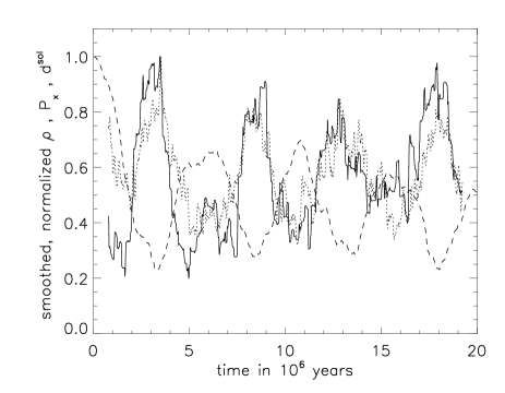
Figure 7: The global oscillation of the slab, if existent, is in antiphase with the modulation of the running mean in time (time window 1.5 Myr) of the Poynting-flux and the density at the central plane of the slab. Shown are, as a function of time in $10^{6}$ years, the normalized spatial extension of the slab (dashed line), and the normalized running mean in time of the Poynting-flux (dotted line) and of the density (solid line). Normalized means that the quantities were divided by the maximum value they assume in the time interval shown.

This rough procedure does not make justice of the specific profile of $\rho_{\mathrm{e}}(x)$. To take care of this, we introduce numerical coefficients, $\alpha_{\mathrm{1}}$, $\alpha_{\mathrm{2}}$, $\alpha_{\mathrm{3}}$, $\alpha_{\mathrm{4}}$, all positive and of order unity. From Eq. 11, the dispersion relation is expected to be of the form:

$$\omega^{2}=\alpha_{\mathrm{1}}\ c_{\mathrm{s}}^{2}k^{2}+\alpha_{\mathrm{2}}\ \frac{v_{\mathrm{\perp}e0}^{2}}{2}k^{2}-\alpha_{\mathrm{3}}\ 4\pi G\rho_{\mathrm{e0}}+\alpha_{\mathrm{4}}\frac{ikv_{\mathrm{\perp}e0}^{2}}{2H_{\mathrm{e}}}.$$ (13)

The last, imaginary, term of Eq. 13 represents the last term of Eq. 11, associated with the modulation of the wave energy flux. For the fundamental mode, $k\approx H_{\mathrm{e}}^{-1}$. Its frequency should then be given by an expression of the form:

$$\omega^{2}=4\pi G\rho_{\mathrm{e0}}\left(\alpha_{\mathrm{1}}\ \frac{c_{\mathrm{s}}^{2}}{c^{2}}+\alpha_{\mathrm{2}}\ \frac{v_{\mathrm{\perp}e0}^{2}/2}{c^{2}}-\alpha_{\mathrm{3}}+i\alpha_{\mathrm{4}}\ \frac{v_{\mathrm{\perp}e0}^{2}/2}{c^{2}}\right),$$ (14)

where $c^{2}=c_{\mathrm{s}}^{2}+v_{\mathrm{\perp}e0}^{2}/2$. This shows that the fundamental time must be, to within a factor of order unity but presumably smaller due to the presence of the negative term $-\alpha_{\mathrm{3}}$, the Jeans frequency $(4\pi G\rho_{\mathrm{e0}})^{1/2}$. From Eq. 12, the associated time is, for $c_{\mathrm{s}}<<v_{\mathrm{e0\perp}}$, of order of $\sqrt{2}H_{\mathrm{e}}/v_{\mathrm{e0\perp}}$. Given the uncertainty left by this analysis on the unknown factors $\alpha_{\mathrm{1}}$ - $\alpha_{\mathrm{4}}$, this is in rough agreement with the results of our simulations. The modulation of the Alfvén flux injected in the slab, caused by the modulation of the central density perturbation, $\rho_{\mathrm{1}}(0)$, constitutes a feedback which endows $\omega^{2}$ with an imaginary part, and thus induces instability, even when the system is stable under constant Alfvén wave energy flux. It is interesting to note that such a modulation is indeed present in our simulations. The coherent oscillations observed in our calculations may represent a nonlinear state of development of such an instability. At high amplitude, the oscillations of the different fluid elements would cease to be isochronic and their initial coherence may be lost.

Figure 8: Good enough spatial resolution is crucial to observe the structuring and supporting effect of the injected Alfvén-wave. Shown is the same simulation, R20.20.5.4.10, once, a), with our usual spatial resolution of 5000 cells and once, b), with a reduced resolution of only 1000 cells. Logarithmic particle density is shown as a function of space (x-axis, in units of 6 pc) and time (y-axis, in units of $10^{6}$ years). A similar loss of structuring and support we observe if the order of the integration scheme is reduced.

5.3 Driving of turbulence and size of structure

The one-point forcing we apply in our simulations is in contrast to most other investigation of highly compressible turbulence, where the forcing is applied at each grid point (see e.g. MacLow (1999) for a description of such forcing and Gammie & Ostriker (1996) for the particular case of a 1D-slab). Our results show that also such one point forcing is perfectly capable of supporting and structuring a slab over large distances. The injected waves are very efficient in distributing the driving energy over a large spatial range.

For the distance over which the injected energy is spread, as well as for the scale of the density structure that forms, the driving wave-length $\lambda_{\mathrm{A0}}$ is decisive. This is not too surprising. In Sect. 3 we have seen that there is no other small length scale likely to play a role in the problem we consider. It then appears quite natural that $\lambda_{\mathrm{A0}}$ governs the structure size. Remembering that smaller scale structure means more inhomogeneity on a smaller spatial scale, a faster destruction of the injected energy for smaller $\lambda_{\mathrm{A0}}$ also seems natural.

That local energy injection can be sufficient to drive turbulence in a whole volume has also been reported for the case of the interaction zone of hypersonically colliding flows in 2D plane-parallel hydrodynamics (Walder & Folini 1998, 2000). Although energy there is injected only at the oblique shocks confining the interaction zone, supersonic turbulence persists in the whole volume. A correlation between driving wave-length and structure size exists as well (Folini & Walder, in preparation). A correlation between structures size and the wave-length of the driving was also reported by MacLow (1999) for hydrodynamic turbulence in a 3D periodic box, which was monochromatically forced at each grid point.

5.4 Numerical resolution

We have experimented with different spatial resolutions and different orders of integration for the MHD equations. Not surprising, we find that simulations with shorter wave-lengths of the Alfvén waves are more delicate in terms of spatial resolution and order of integration. For run R20.20.5.4.10 we have verified that our results remain essentially unchanged (mean quantities differ by a few percent at most) if we further increase the spatial resolution. For coarser discretizations (using 1000 cells instead of 5000) or lower orders of integration, strong damping of the Alfvén wave due to numerical diffusion occurs and both the density substructure as well as the additional support against self-gravity are essentially lost, as can be seen in Fig. 8. For run R20.20.5.4.10, for example, $\langle d^{\mathrm{sol}}/d_{\mathrm{0}}^{\mathrm{wkb}}\rangle_{\mathrm{t}}$ is reduced from 0.46 to 0.32, for run R20.20.10.4.10 the value is reduced from 0.75 to 0.48. With regard to numerical simulations, these results show that the problem we investigated in this paper is currently out of reach for 3D simulations.

5.5 Connection to high density cores

We, finally, would like to return to the larger frame, molecular clouds and the formation of dense cores. As mentioned earlier, both theoretical and observational results today indicate that the immediate vicinity of a forming dense core is highly structured. Most striking are the observations by Falgarone et al. (2001) of the filaments around the starless dense core L1512. Various explanations for their existence, all employing magnetic fields, seem plausible (Fiege & Pudritz 2000; Franqueira et al. 2000; Del Zanna et al. 2001). It seems most likely that such structures, or rather the responsible physical processes, affect the formation and accretion rate of dense cores.

Detailed studies of this structuring and its consequences are mandatory to better link turbulence in molecular clouds with star formation. Such studies are, however, only at their beginning. The 1D slab we studied here is by no means an accurate model of a molecular cloud. Nevertheless, it shows that magnetic waves can play a crucial role in counteracting self-gravity. The 3D grid studies by Heitsch et al. (2001), mentioned in the introduction, point in the same direction. And while the 2D and 3D MHD simulations by Del Zanna et al. (2001) of a plan parallel slab focus on structure formation rather than on accretion, they show that density filaments form, more or less aligned with the background magnetic field.

With regard to future simulations in this field, existing simulations show spatial resolution to be decisive. Another crucial issue is dimensionality. The ’fingering’ observed by Del Zanna et al. (2001) - and by Falgarone et al. (2001) - clearly cannot be studied in a 1D model. And, as the authors showed as well, it can only be observed if open boundaries are used, not periodic ones. Finally, and probably most crucial of all, a future model of dense core formation will have to account for the generation of magnetic waves self-consistently. This may be the strongest reason to aim, in a next step, at multidimensional models.

6 Conclusions

For the case of a 1D plane-parallel, self-gravitating slab we have shown by means of numerical simulations and dimensional analysis the following:

1) One source of energy injection is sufficient to sustain turbulence throughout the slab.

2) The time-averaged spatial extension of the turbulent slab is comparable to the extension of the corresponding WKB solution. Deviations are at most a factor of three and depend about linearly on the ratio of the initial central Alfvén wave-length and the extension of the WKB solution.

3) The scale of the substructure is governed by the initial central Alfvén wave-length and the temperature. Larger wave-lengths and smaller temperatures lead to larger scale structure.

4) The energy loss, and thus the energy radiated by the slab, is dominated by the loss of Poynting-flux, which increases almost linearly with $\sqrt{\beta_{\mathrm{0}}}$.

5) Within the slab, the energy density of the transverse magnetic field and the kinetic energy density of the transverse velocities are in approximate equilibrium. The latter accounts for between 70% and 90% of the total kinetic energy density.

(6) A too coarse mesh or a low order scheme leads to substantial wave-damping, thus to loss of structuring and support.

Appendix A Simulation parameters

Table 1: The parameters used in the different simulations. The first column contains the name of each run. These names reflect the free parameters of each run. For example, R20.10.25.4.40 is the simulation with $B_{\mathrm{\parallel}}=20\mu$G, $B_{\mathrm{\perp}}=10\mu$G, $2\pi/\omega=25\cdot 10^{4}$ years, a central density of $N_{\mathrm{0}}=4\cdot 250$ particles per cm³, and $T=40$K. Subsequent columns, from left to right, denote: $\lambda_{\mathrm{A0}}=c_{\mathrm{A0}}2\pi/\omega$: initial central Alfvén wave-length in $2.176\cdot 10^{17}$ cm; ${\cal M}_{\mathrm{0}}/(m_{\mathrm{H}}{\cal D})$: initial mean particle density in cm^-3; ${\cal M}_{\mathrm{0}}/{\cal M}^{\mathrm{\infty}}_{\mathrm{0}}$: ratio of column densities within computational domain and in infinite space of initial WKB solution; $d^{\mathrm{wkb}}_{\mathrm{0}}/d^{\mathrm{hs}}_{\mathrm{0}}$: ratio of extensions of WKB and hydrostatic solution at $t=0$; $d^{\mathrm{wkb}}_{\mathrm{0}}/{\cal D}$: spatial extension of initial WKB solution in units of computational domain; $\alpha_{\mathrm{0}}=B_{\mathrm{\perp}}^{2}/B_{\mathrm{\parallel}}^{2}$: dimensionless parameter; $\beta_{\mathrm{0}}=2c_{\mathrm{s}}^{2}/c_{\mathrm{A0}}^{2}$: central, initial plasma beta; $W_{\mathrm{0}}=\omega/\sqrt{2\pi G\rho_{\mathrm{0}}}$: WKB parameter; $W_{\mathrm{\lambda A0}}=\lambda_{\mathrm{A0}}/d^{\mathrm{wkb}}_{\mathrm{0}}$: alternative WKB parameter; $\langle d^{\mathrm{sol}}\rangle_{t}/{\cal D}$: time averaged spatial extension of solution, average taken between $5\cdot 10^{6}$ years and $2\cdot 10^{7}$ years, in units of total domain ${\cal D}$; $\langle d^{\mathrm{sol}}\rangle_{t}/d^{\mathrm{wkb}}_{\mathrm{0}}$: ratio of time averaged spatial extension of solution and extension of corresponding, initial WKB solution; $\sigma_{\mathrm{d}}^{\mathrm{rel}}$: relative standard deviation of $d^{\mathrm{sol}}(t)/d^{\mathrm{wkb}}_{\mathrm{0}}$; ${\cal M}_{\mathrm{20}}/{\cal M}_{\mathrm{0}}$: ratio of the column densities at times $t=20\cdot 10^{6}$ years and $t=0$; $\Delta P$: time averaged, percental change of Poynting-flux between central plane and $\langle d^{\mathrm{sol}}\rangle_{\mathrm{t}}$ in units of the initial WKB Poynting-flux, $\Delta P=100\cdot{\langle\Delta P^{\mathrm{sol}}_{\mathrm{x}}\rangle_{t}}/P_{\mathrm{x0}}$.

run	$\lambda_{\mathrm{A0}}$	$\frac{{\cal M}_{\mathrm{0}}}{m_{\mathrm{H}}{\cal D}}$	$\frac{{\cal M}_{\mathrm{0}}}{{\cal M}^{\mathrm{\infty}}_{\mathrm{0}}}$	$\frac{{d}^{\mathrm{wkb}}_{\mathrm{0}}}{{d}^{\mathrm{hs}}_{\mathrm{0}}}$	$\frac{{d}^{\mathrm{wkb}}_{\mathrm{0}}}{\cal D}$	$\alpha_{\mathrm{0}}$	$\beta_{\mathrm{0}}$	$W_{\mathrm{0}}$	$W_{\mathrm{\lambda A0}}$	$\frac{\langle{d}^{\mathrm{sol}}\rangle_{t}}{{\cal D}}$	$\frac{\langle{d}^{\mathrm{sol}}\rangle_{t}}{{d}^{\mathrm{wkb}}_{\mathrm{0}}}$	$\sigma_{\mathrm{d}}^{\mathrm{rel}}$	$\frac{{\cal M}_{\mathrm{20}}}{{\cal M}_{\mathrm{0}}}$	$\Delta P$
R100.45.1.4.10	1	195	0.30	14.3	0.37	0.20	0.0035	750.	0.032	0.12	0.32	0.24	1.02	6.9
R100.45.5.4.10	5	195	0.30	14.3	0.37	0.20	0.0035	150.	0.16	0.38	1.02	0.74	0.89	5.3
R100.45.5.8.10	3.5	220	0.34	9.9	0.23	0.20	0.0069	110.	0.18	0.33	1.43	0.76	0.96	7.3
R100.20.1.4.10	1	116	0.38	5.5	0.24	0.04	0.0035	750.	0.049	0.12	0.50	0.22	1.02	5.3
R100.20.5.4.10	5	116	0.38	5.5	0.24	0.04	0.0035	150.	0.24	0.41	1.71	0.90	0.92	4.2
R100.10.5.4.10	5	82.1	0.45	2.6	0.16	0.01	0.0035	150.	0.37	0.30	1.88	0.77	1.02	3.6
R50.45.10.8.10	3.5	220	0.34	9.9	0.23	0.81	0.028	53.	0.18	0.32	1.39	0.52	0.93	2.6
R20.20.5.4.10	1	116	0.38	5.5	0.24	1.00	0.087	150.	0.045	0.11	0.46	0.14	1.02	21.
R20.20.10.4.10	2	116	0.38	5.5	0.24	1.00	0.087	75.	0.098	0.18	0.75	0.20	1.00	19.
R20.20.12.4.10	2.5	116	0.38	5.5	0.24	1.00	0.087	60.	0.12	0.18	0.75	0.12	1.02	20.
R20.20.17.4.10	3.5	116	0.38	5.5	0.24	1.00	0.087	43.	0.17	0.25	1.04	0.24	0.99	17.
R20.20.25.4.10	5	116	0.38	5.5	0.24	1.00	0.087	30.	0.24	0.34	1.42	0.30	0.98	19.
R20.20.25.8.10	3.5	136	0.42	3.8	0.14	1.00	0.17	21.	0.30	0.18	1.39	0.88	1.02	22.
R20.20.5.1.10	2	85.7	0.30	9.7	0.57	1.00	0.022	300.	0.041	0.23	0.40	0.85	0.99	13.
R20.10.5.4.10	1	82.1	0.45	2.6	0.16	0.25	0.087	150.	0.073	0.11	0.68	0.09	1.02	19.
R20.10.25.4.10	5	82.1	0.45	2.6	0.16	0.25	0.087	30.	0.37	0.24	1.50	0.42	1.01	13.
R20.10.2.1.10	1	56.4	0.37	4.8	0.43	0.25	0.022	600.	0.027	0.20	0.47	0.19	0.99	12.
R20.10.5.1.10	2	56.4	0.37	4.8	0.43	0.25	0.022	300.	0.055	0.24	0.56	0.13	0.99	11.
R20.10.12.1.10	5	56.4	0.37	4.8	0.43	0.25	0.022	120.	0.14	0.42	0.98	0.15	0.93	10.
R20.20.5.4.5	1	102.	0.35	8.7	0.22	1.00	0.043	150.	0.053	0.09	0.41	0.15	1.03	19.
R20.20.5.4.20	1	135.	0.41	3.6	0.27	1.00	0.17	150.	0.044	0.13	0.48	0.13	1.01	25.
R20.20.5.4.40	1	162.	0.44	2.4	0.30	1.00	0.35	150.	0.039	0.18	0.60	0.14	1.02	32.
R20.20.25.4.5	5	102.	0.35	8.7	0.22	1.00	0.043	30.	0.27	0.31	1.41	0.42	0.98	17.
R20.20.25.4.15	5	126.	0.40	4.3	0.26	1.00	0.13	30.	0.23	0.28	1.08	0.22	0.97	17.
R20.20.25.4.20	5	135.	0.41	3.6	0.27	1.00	0.17	30.	0.22	0.26	0.96	0.17	0.96	20.
R20.20.25.4.40	5	162.	0.44	2.4	0.30	1.00	0.35	30.	0.20	0.27	0.90	0.15	0.97	24.
R20.20.25.8.5	3.5	117.	0.38	5.9	0.13	1.00	0.087	21.	0.32	0.20	1.54	0.93	1.05	18.
R20.20.25.8.20	3.5	164.	0.45	2.6	0.16	1.00	0.35	21.	0.26	0.17	1.06	0.27	1.02	29.
R20.20.25.8.40	3.5	205.	0.47	1.8	0.18	1.00	0.69	21.	0.23	0.19	1.06	0.32	1.02	39.
R20.20.5.1.20	2	93.9	0.32	5.7	0.61	1.00	0.043	300.	0.039	0.28	0.46	0.14	0.99	14.
R20.10.5.4.5	1	68.2	0.42	3.8	0.14	0.25	0.043	150.	0.084	0.10	0.71	0.18	1.02	15.
R20.10.5.4.20	1	102.	0.47	1.8	0.18	0.25	0.17	150.	0.065	0.13	0.73	0.12	1.02	26.
R20.10.25.4.20	5	102.	0.47	1.8	0.18	0.25	0.17	30.	0.33	0.25	1.39	0.45	0.98	17.
R20.10.25.4.40	5	133.	0.49	1.4	0.22	0.25	0.35	30.	0.27	0.28	1.27	0.14	0.99	25.
R20.10.12.1.5	5	49.9	0.34	7.6	0.39	0.25	0.011	120.	0.15	0.46	1.18	0.29	0.94	8.8
R20.10.12.1.20	5	65.5	0.40	3.0	0.47	0.25	0.043	120.	0.13	0.46	0.98	0.11	0.95	13.

References

- Ballesteros-Paredes et al. (1999) Ballesteros-Paredes, J., Hartmann, L., & Vázquez-Semadeni, E. 1999, ApJ, 527, 285
- Barmin et al. (1996) Barmin, A. A., Kulikovsky, A. G., & Pogorelov, N. V. 1996, Journal of Computional Physics, 126, 77
- Barranco & Goodman (1998) Barranco, J. A. & Goodman, A. A. 1998, ApJ, 504, 207
- Bourke et al. (2001) Bourke, T. L., Myers, P. C., & Robinson, G. e. a. 2001, ApJ, 554, 916
- Cho et al. (2002) Cho, J., Lazarian, A., & Vishniac, E. T. 2002, ApJ, 566, L49
- Crutcher (1999) Crutcher, R. M. 1999, ApJ, 520, 706
- Del Zanna et al. (2001) Del Zanna, L., Velli, M., & Londrillo, P. 2001, A&A, 367, 705
- Derby (1978) Derby, N. F. 1978, ApJ, 224, 1013
- Elmegreen (1999) Elmegreen, B. G. 1999, ApJ, 527, 266
- Elmegreen (2000) Elmegreen, B. G. 2000, ApJ, 530, 277
- Falgarone et al. (2001) Falgarone, E., Pety, J., & Phillips, T. G. 2001, ApJ, 555, 178
- Falle & Hartquist (2002) Falle, S. A. E. G. & Hartquist, T. W. 2002, MNRAS, 329, 195
- Fiege & Pudritz (2000) Fiege, J. D. & Pudritz, R. E. 2000, MNRAS, 311, 85
- Franqueira et al. (2000) Franqueira, M., Tagger, M., & Gómez de Castro, A. I. 2000, A&A, 357, 1143
- Fukuda & Hanawa (1999) Fukuda, N. & Hanawa, T. 1999, ApJ, 517, 226
- Gammie & Ostriker (1996) Gammie, C. F. & Ostriker, E. C. 1996, ApJ, 466, 814
- Goldstein (1978) Goldstein, M. L. 1978, ApJ, 219, 700
- Hartmann et al. (2001) Hartmann, L., Ballesteros-Paredes, J., & Bergin, E. A. 2001, ApJ, 562, 852
- Heitsch et al. (2001) Heitsch, F., Mac Low, M., & Klessen, R. S. 2001, ApJ, 547, 280
- Kudoh & Basu (2003) Kudoh, T. & Basu, S. 2003, ApJ, in press, astro–ph/0306473
- Mac Low (2002) Mac Low, M.-M. 2002, in Simulations of magnetohydrodnamic turbulence in astrophysics, ed. T. Passot & E. Falgarone, in press, astro–ph/0201157
- MacLow (1999) MacLow, M.-M. 1999, ApJ, 524, 169
- Malara et al. (2000) Malara, F., Primavera, L., & Veltri, P. 2000, Phys. Plasmas, 7, 2866
- Malara & Velli (1996) Malara, F. & Velli, M. 1996, Phys. Plasmas, 3, 4427
- Martin et al. (1997) Martin, C. E., Heyvaerts, J., & Priest, E. R. 1997, A&A, 326, 1176
- Matthews et al. (2002) Matthews, B. C., Fiege, J. D., & Moriarty-Schieven, G. 2002, ApJ, 569, 304
- Matthews & Wilson (2002) Matthews, B. C. & Wilson, C. D. 2002, ApJ, 571, 356
- Palla & Stahler (2000) Palla, F. & Stahler, S. W. 2000, ApJ, 540, 255
- Pruneti & Velli (1997) Pruneti, F. & Velli, M. 1997, in Fifth SOHO Workshop: The Corona and Solar Wind Near Minimum Activity, 623–627
- Spitzer (1968) Spitzer, L. 1968, Diffuse Matter in Space (Interscience Publisher)
- Strang (1968) Strang, G. 1968, SIAM J.Num.Anal., 5, 506
- Turkmani & Torkelsson (2003) Turkmani, R. & Torkelsson, U. 2003, A&A, in press, astro–ph/0307559
- Walder & Folini (1998) Walder, R. & Folini, D. 1998, A&A, 330, L21
- Walder & Folini (2000) Walder, R. & Folini, D. 2000, in Thermal and Ionization Aspects of Flows from Hot Stars: Observations and Theory, ed. H. J. G. L. M. Lamers & A. Sapar, ASP Conference Series, 281–285
- Walder & Folini (2000) Walder, R. & Folini, D. 2000, Ap&SS, 274, 343
- Ward-Thompson et al. (2000) Ward-Thompson, D., Kirk, J. M., & Crutcher, R. M. e. a. 2000, ApJ, 537, L135