A Deep, High-Resolution Survey at 74 MHz

Abstract

We present a 74 MHz survey of a 165 square degree region located near the north galactic pole. This survey has an unprecedented combination of both resolution ($25^{\prime\prime}$ FWHM) and sensitivity ($\sigma$ as low as 24 mJy/beam). We detect 949 sources at the $5\sigma$ level in this region, enough to begin exploring the nature of the 74 MHz source population. We present differential source counts, spectral index measurements and the size distribution as determined from counterparts in the high resolution FIRST 1.4 GHz survey. We find a trend of steeper spectral indices for the brighter sources. Further, there is a clear correlation between spectral index and median source size, with the flat spectrum sources being much smaller on average. Ultra-steep spectrum objects ($\alpha\leq-1.2$; $S_{\nu}\propto S^{\nu}$) are identified, and we present high resolution VLA follow-up observations of these sources which, identified at such a low frequency, are excellent candidates for high redshift radio galaxies.

1 Introduction

The new 74 MHz system on the Very Large Array (VLA), fully implemented in 1998 (Kassim et al., 1993), has opened a new window into the previously unexplored regime of very low frequency radio observations at high sensitivity and sub-arcminute resolution.

The radio source population at very low frequencies is of interest for several reasons. Samples selected at $\nu\sim 74$ MHz are completely dominated by isotropic radio emission, unlike those found at higher frequencies, where orientation-dependent Doppler boosting enhances the observed emission for some fraction of sources: even for the 178 MHz 4C survey (Pilkington & Scott (1965); Gower, Scott, & Wills (1967)) 10% of sources were significantly affected by Doppler beaming (Wall & Jackson, 1997), leading to biased samples of radio sources where those sources with jets pointing toward us are relatively over represented. In addition, at frequencies below 100 MHz spectral curvature is much more common than at higher frequencies, providing an important tool for studying the properties of the absorbing gas. This is because at low frequencies, the needed optical depths for absorption due to free-free absorption by H ii regions (intrinsic or intervening) or synchrotron self-absorption require lower electron densities than at higher frequencies.

The ability to find steep spectrum sources is of value because of its relative efficiency in finding very high redshift radio galaxies ($z>2$). Identifying ultra-steep spectrum sources has now been used by many groups for a number of years to find the highest redshift radio galaxies (Röttgering et al., 1994; Chambers et al., 1996; Blundell et al., 1998). This method has been implemented mainly with frequencies above 150 MHz (De Breuck et al. (2000), Blundell et al. (1998)), and is based on the curved nature of the radio spectral energy distribution. Most low-redshift radio galaxies have spectra that flatten below 325 MHz, while the higher redshift objects are observed at a higher rest frame frequency, where the SED is steep. At 74 MHz, this method is likely to be even more efficient, since the spectra of most low-redshift radio galaxies will have flattened to a much greater degree at this very low frequency, increasing the contrast between them and the high redshift radio galaxies.

Although radio galaxies are no longer the only galaxies found at the very highest redshifts (Hu et al., 2002; Kodaira et al., 2003; Cuby et al., 2003) and certainly not the most abundant high-redshift galaxies (Steidel et al., 1996, 1999) they do have unique characteristics: (1) the selection via radio emission means that radio-loud AGN are selected free of caveats concerning dust, which is probably a very important factor in the high-redshift Universe, as is evidenced by the huge sub-millimeter luminosities associated with radio galaxies at high redshift (e.g. Archibald et al. 2001; Reuland et al. 2003) (2) their strong narrow-emission lines allow relatively simple redshift determinations that do not rely on stellar continuum breaks or absorption lines and (3) powerful ($L_{151}>10^{25}$ W m^-2 Hz^-1) radio galaxies inhabit some of the most massive galaxies in the Universe at all cosmic epochs (Jarvis et al., 2001; De Breuck et al., 2002; Willott et al., 2003), and as such provide a unique probe into the build-up of massive galaxies. With the recent work on the correlation between black-hole mass and bulge luminosity in the local Universe (Magorrian et al., 1998), the fact that galaxies which exhibit powerful radio emission are the most massive means they probably host the the most massive black holes (Dunlop et al., 2003; Bettoni et al., 2003). The evidence for super-massive black holes in the centers of all bulge dominated galaxies also implies that every massive galaxy in the local Universe may have had an active phase in the past. This is further reinforced by the similarity in number density of super-massive black holes in the local Universe and the density of quasars at $z\sim 2.5$, i.e. the quasar epoch. Thus, we may need to understand AGN activity to understand massive galaxy formation in general.

A further characteristic of radio galaxies is, by definition, their radio emission. This allows a unique estimate of the time since the radio AGN was triggered (Blundell, Rawlings, & Willott, 1999), and it enables us to probe the gaseous environment via Faraday rotation measures (Carilli et al., 1997). But possibly more importantly in the years to come, it allows us to probe 21 cm HI absorption along the line-of-sight to the radio source. This will be vitally important as 21 cm absorption (and emission) will allow us to probe the epoch of reionization. These studies will be tractable with the development of the new era of radio telescopes such as the LOFAR (Kassim et al., 2000) and the SKA which will have the sensitivity to probe such a signal. Radio sources that are placed at the epoch before which the reionization is fully completed will be a very important probe of this epoch, allowing the study of the neutral gas at parsec and kiloparsec scales. Such scales are much smaller than are being probed by WMAP or Plank. Thus, it is crucial to find radio sources at $z>6$ to allow these investigations to take place, and selecting ultra-steep spectrum (USS) radio sources is a well proven technique for finding the highest-redshift radio galaxies (Rawlings et al., 1996; van Breugel et al., 1999), and selecting at 74 MHz allows us to do this better than ever before.

In this paper, we describe the survey with a discussion of observational methodology in Section 2 and the mapping results and source extraction in Section 3. In Section 4 we explore the nature of the 74 MHz radio source population. In Section 5, we identify the ultra-steep spectrum sources and present high-resolution follow-up radio observations to determine their identities.

2 Observational Methodology

2.1 The Data Set

The data used to produce this survey comes from observations taken on March 7, 1998, intended to map two normal galaxies at 74 MHz (NGC 4565 and NGC 4631). Though these two targets were largely resolved out at this resolution, the combination of A-configuration resolution, favorable ionospheric conditions and pointings near the north galactic pole where the background temperature is low produced the deepest observation ever obtained below 100 MHz. That the two fields observed were separated by $6.4^{\circ}$, which is roughly the radius of the primary beam at 74 MHz, allowed the two fields to be ideally combined to produce a single deep image of an area roughly $17^{\circ}\times 10^{\circ}$ in size.

The data was taken in spectral line mode to reduce bandwidth smearing and to facilitate removal of radio frequency interference. The total bandwidth of 1.54 MHz was divided into 128 channels, which Hanning smoothing reduced to 64. The central frequency was 73.8 MHz and the integration time was 10 seconds. Each of the two pointings was observed for 3 hours, and the observation alternated between the two fields to better distribute the $uv$-coverage.

2.2 Challenges for High Resolution Imaging at Low Frequency

There are many challenges to high resolution imaging at low radio frequencies which have prevented this observational regime from being explored until the past few years. In this section, we summarize these issues and their solutions. Kassim et al. (2003) provide a more comprehensive description of 74 MHz observations with the VLA. In addition, a low frequency data reduction tutorial is available online .

2.2.1 Radio Frequency Interference

The monitor and control system of the VLA generates significant radio frequency interference (RFI) below 100 MHz, and there is the potential for external RFI as well. For this reason (and others) the data are acquired in spectral-line mode. Excision of potential RFI is performed on a per-baseline basis for each visibility sample. Actual excision is accomplished by correcting the spectral-line data for the shape of the VLA bandpass at this frequency, fitting a linear baseline, then flagging any data exceeding a level typically set to be 6–8 times the expected rms noise level. Typically this procedure removes 10-15% of the visibility data. It is notable, however, that at 74 MHz there is no evidence to indicate that any of this RFI is externally generated.

2.2.2 The “3-D Problem”

One crucial aspect for the post processing of these data sets is the need for a three-dimensional inversion of the visibility data. A conventional two-dimensional inversion of the three-dimensional visibility function, as measured by a non-coplanar (i.e., non–east-west) array like the VLA, introduces errors in the image plane which increase as the square of the distance from the phase center. The “3-D” problem becomes severe at long wavelengths where the primary beam is large and contains hundreds of discrete sources which must be properly deconvolved to achieve thermal-noise– or classical-confusion–limited maps.

To solve this problem, Cornwell & Perley (1992) have developed a polyhedron algorithm in which the three-dimensional “image volume” is approximated by many two dimensional “facets,” small enough that the traditional two-dimensional assumption is valid. Thus a “fly’s eye” of small overlapping images, each with its own phase center, is made to cover the large field of view. Typically, many hundreds of facets are needed to map the full primary beam area, and after cleaning and imaging, these images are then combined into a single undistorted image of the full field of view.

2.2.3 Ionospheric Image Distortion

The biggest challenge to achieving high resolution at low frequencies is the distortion of phases caused by the ionosphere, an effect which increases proportionally with wavelength (Kassim et al., 1993). This problem is compounded by the fact that the field of view at 74 MHz is so large, that these phase distortions can vary significantly across the field of view. This puts phase calibration of 74 MHz data into an entirely different regime from higher frequencies in which all phase distortions can be completely described by a single time-variable number for each antenna. For this reason, traditional self-calibration does not apply. Rather, a field-based calibration method, in which the phase calibration is position-dependent, is needed. Such an algorithm has been written by J. J. Condon and W. D. Cotton (Cotton & Condon, 2002). This algorithm models the ionosphere as phase screen varying in space and time, and applies a two-dimensional Zernike polynomial phase correction to correct the phases across the entire field of view.

2.3 Data Reduction

Cygnus A (3C405) was used for bandpass and amplitude calibration. Phase calibration was more complicated. As described in section 2.2.3, calibration which applies a constant phase correction to the entire field is insufficient for imaging of the entire 74 MHz VLA primary beam, and field-based calibration is needed. However, an initial calibration estimate is necessary to begin the field-based calibration, and so as a first step, we calibrated the field to a sky model obtained using the 1.4 GHz NVSS catalog (Condon et al., 1998) adjusted for a spectral index of $\alpha=-0.75$. Next, field-based calibration was used to remove ionospheric smearing before imaging and cleaning were performed. The field-based calibration was performed with a time resolution of 2 minutes, enough to significantly detect an average of 6 to 10 sources in the field of view. Each pointing was mapped to a radius of $6^{\circ}$ using roughly 300 facets. We used a pixel size of $7.5^{\prime\prime}$ and each facet was 360 pixels in diameter. A circular $25^{\prime\prime}$ restoring beam was used. The images from the two fields were then corrected for the primary beam shape, and co-added to produce a single image.

3 Results

3.1 Image Quality

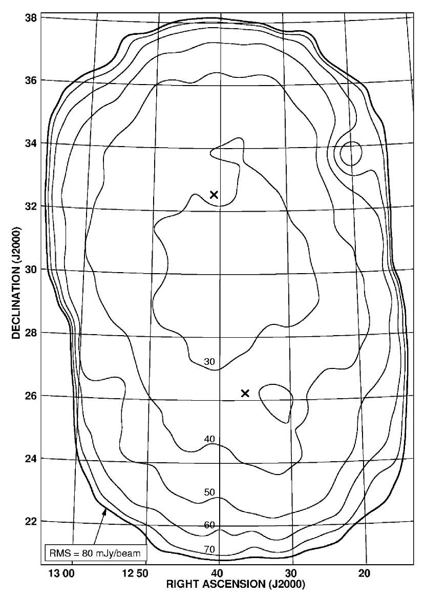
Figure 2: Noise levels in the 74 MHz survey area as determined by local measuments of the RMS noise in the image. The contours plotted are at 30, 40, 50, 60, 70 and 80 mJy/beam, with the outermost contour at 80 mJy/beam in bold defining the boundary of the survey. Each of the two field centers is marked with an “X”.

Our final image has a resolution of $25^{\prime\prime}$ and a minimum RMS noise level of 24 mJy/beam, a unique combination for such a low frequency survey (see Figure 1). However, the noise level varies over the image due to the primary beam sensitivity patterns for the two fields, the added sensitivity due to the two fields overlapping and occasional incompletely cleaned sidelobes from bright sources (Figure 2). The image has no real “edge”, just an increase in the noise level with distance from the pointing centers. If we define the survey area as the area in our map for which the RMS noise is lower than a set limit, then as this limit is increased the survey area increases. However, at points more than about $5^{\circ}$ from either pointing center the noise level begins to increase so rapidly that the benefits of increasing the survey area quickly diminish (see Table 1). We chose the field edge to be at the 80 mJy/beam noise level, which defines a total survey area of 165.1 square degrees, with almost half of this area having a sensitivity below 40 mJy/beam.

3.2 Source Extraction

The same algorithm which was written for use in the 1.4 GHz NVSS (Condon et al., 1998) was used to identify and characterize sources in this 74 MHz survey survey. This algorithm works by identifying “islands” of emission in the image above a set threshold and fitting each source to a model of up to four Gaussians. We set as our source detection threshold that sources must have both a peak and integrated flux level at least 5 times the local RMS noise level. Therefore, the source detection threshold varies over the image as the RMS noise varies.

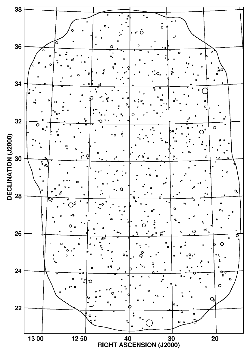
Figure 3: Location of all sources identified at the $5\sigma$ level within the survey region. The area of each circle is proportional to the integrated flux of that source. The weakest source is 146 mJy and the strongest is 39.9 Jy.

We combined into multiple sources (sources composed of more than one Gaussian component), those sources located within $120^{\prime\prime}$ of each other. This distance was chosen because it corresponds to the separation distance of radio sources for which doubles which are components of the same source (usually a radio galaxy) outnumber those that are actually two separate objects by a ratio of 10 to 1 as determined by a recent study of the clustering of radio sources in the NVSS (Overzier et al., 2003). In total, we detected 949 sources (Figure 3) with integrated fluxes ranging from 146 mJy to 39.9 Jy. Of these, 70 were multiple sources. Most sources were not much larger than the $25^{\prime\prime}$ beamsize, with only 75 sources (7.9%) measuring larger than two beamwidths across, either as the fitted size of a single source or the maximum separation within a multiple source. Most of the extended sources appear to be FRII type radio galaxies. Figure 4 shows contour maps of the 80 largest sources in the survey. The complete catalog of all sources is available in the electronic edition of the Astrophysical Journal in Table 2.

4 Source Statistics

4.1 Source Counts

We present Euclidean-normalized differential source counts in Figure 5. These were calculated within flux density bins of size $\pm 15\%$ from the central flux density. To ensure a true measure of source densities, for each flux density bin we only considered the region of the survey in which all sources in that flux density bin are detected with at least $7\sigma$ confidence, the canonical level of $2\sigma$ completeness for sources selected above a $5\sigma$ threshold. Thus, for each flux density bin we only selected sources from the region of the survey with a noise level lower than 1/7 of the lower flux density limit of that bin. The source density was calculated by dividing this source count by the area of that “$7\sigma$” region from which the sources were selected.

Also plotted in Figure 5 is a polynomial fit to the source count at 327 MHz (Wieringa, 1991) and its adjustments according to various spectral indices. The data at 74 MHz seems to correspond to an average spectral index of somewhere between $\alpha=-0.5$ and $\alpha=-0.75$, though there seems to be an overall trend of steeper corresponding spectral index at higher flux levels. We caution that this is not a direct measurement of the average spectral index as many compact sources seen at 327 MHz are not seen at 74 MHz due to synchrotron self-absorption.

We note that the differential source counts function depends to some degree on our choice of spatial cutoff for grouping sources. Though we grouped components closer than $120^{\prime\prime}$ into single sources, if larger physical sources were broken into multiple “sources”, the differential source counts function would be artificially increased for lower flux densities and decreased for the highest flux densities. However, this effect is likely to be minor. For example, if we double the spatial cutoff to $240^{\prime\prime}$, only 35 additional sources ($3.7\%$) are “grouped”. Further, it is unlikely that all of these new multiple sources are physical, with (Overzier et al., 2003) predicting near parity between physical and coincidental doubles at a spacing of $240^{\prime\prime}$.

4.2 Comparisons to Other Survey Catalogs

We compared our source catalog to the 1.4 GHz NVSS catalog (Condon et al., 1998) which, with its resolution of $45^{\prime\prime}$, is well enough matched to our resolution to provide accurate spectral index measurements. The long frequency interval between 74 MHz and 1.4 GHz also contributes to the accuracy of the spectral index measurements as a flux ratio error of 10% produces a spectral index error of only $\Delta\alpha=0.032$. We found NVSS matches within $60^{\prime\prime}$ for 947 out of our total of 949 sources. The two sources without NVSS matches were J1230.6+3247 and J1253.6+2509, implying very steep spectral index upper limits of $-1.47$ and $-1.78$ respectively. It is therefore reasonable to wonder if these are real detections. The peak flux density of J1230.6+3247 was measured to be 188 mJy/beam, which is a $6.3\sigma$ detection given the local noise level of 29.8 mJy/beam. This relatively strong detection and the fact that the spectral index necessary to explain the lack of detection is, though very steep, not even the steepest in the survey, lead us to conclude that this source is probably real. The peak flux density of J1253.6+2509 was measured to be 256 mJy/beam, which was just barely over our $5\sigma$ detection threshold for the local noise level of 50.4 mJy/beam. Because of this and the extraordinary steepness of its spectrum necessary to explain its lack of detection by NVSS, we conclude that it is a non-negligible possibility that this may be a false detection. However, as it meets our criteria for a source detection, we still include it in our source list.

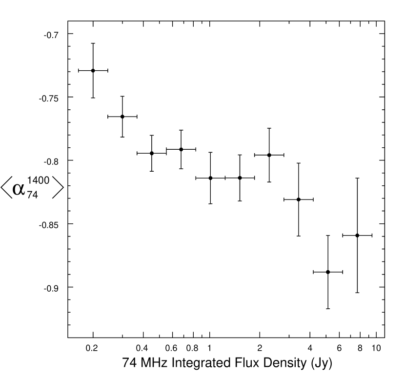
Figure 7: Mean spectral index versus 74 MHz flux density. The horizontal error bars correspond to the bin widths.

We present the spectral index measurements in Figure 6 plotted versus the integrated flux density at 74 MHz. The spectral indices of all sources with respect to their NVSS counterparts are included in the source catalog, available electronically. We find a median spectral index of $\alpha=-0.79$. Figure 7 shows the spectral index as a function of 74 MHz flux density, and it is clear that the average spectral index steepens with increasing flux density.

In addition to the spectral index between the widely spaced frequencies of 74 MHz and 1.4 GHz, it is of interest to investigate the actual shape of the spectrum within this interval. For this, we turn to the 327 MHz WENSS survey (Rengelink et al., 1997). Although the WENSS only covers the northern sky down to a declination of $+29^{\circ}$, which falls near the middle of our survey region, we find counterparts (within $60^{\prime\prime}$) to 545 sources. Figure 9 shows a comparison of the spectral indices for two frequency intervals in the form of a radio color-color plot. As this plot shows, most source spectra flatten considerably from the “low” frequency interval from 327 MHz to 1.4 GHz to the “very low” frequency interval from 74 MHz to 327 MHz. Quantitatively, we found a median change in the spectral index of $\Delta\alpha=0.24$.

We also compared our source catalog to the higher resolution ($5.4^{\prime\prime}$) 1.4 GHz FIRST survey (White et al., 1997). We found matches within $30^{\prime\prime}$ for 945 out of our total of 949 sources (including neither of the 2 sources without NVSS matches). This allowed a much better measurement of source sizes than was possible with the $25^{\prime\prime}$ resolution of the 74 MHz observations. We define the source size as either the deconvolved major axis for single sources in FIRST or as the maximum separation between components for the multiple sources. Overall, we find a median source size of $8.1^{\prime\prime}$, though we notice a strong correlation between source size and spectral index. Figure 8 shows the median source size as a function of spectral index along with a spectral index histogram. It is clear that the steeper the spectrum the larger the sources, which makes sense as one would expect compact sources to have flatter spectra on average due to synchrotron self-absorption, although this trend seems to stall if not reverse for the very steep spectrum objects ($\alpha<-1$).

5 Ultra Steep Spectrum Sources

5.1 Identification and Follow-up

To identify our sample of ultra-steep spectrum (USS) sources, we chose a spectral index cutoff of $\alpha_{74}^{325}<-1.2$. With this criterion, we identified 26 USS sources out of a total of 949 sources (2.7%). This included 24 sources with measured spectral indices and the 2 sources with no FIRST or NVSS counterparts which have spectral index upper limits which qualify them as USS as well.

This percentage of USS sources is much higher than that found in the previous USS searche by De Breuck et al. (2000) which found a USS fraction of only 0.5%. Even if we use their stricter USS criteria of $\alpha<-1.3$, we still have detected 18 USS sources, or 1.9%. It is unclear exactly what causes this difference, but it is possibly due to a combination of effects. First, by selecting sources at 74 MHz, rather than 325, we have eliminated virtually the entire population of flat spectrum objects from our sample. Second, as 74 MHz observations are less sensitive than those at higher frequencies, we have a brighter sample, and it is known that as the flux limit increases, the USS fraction increases.

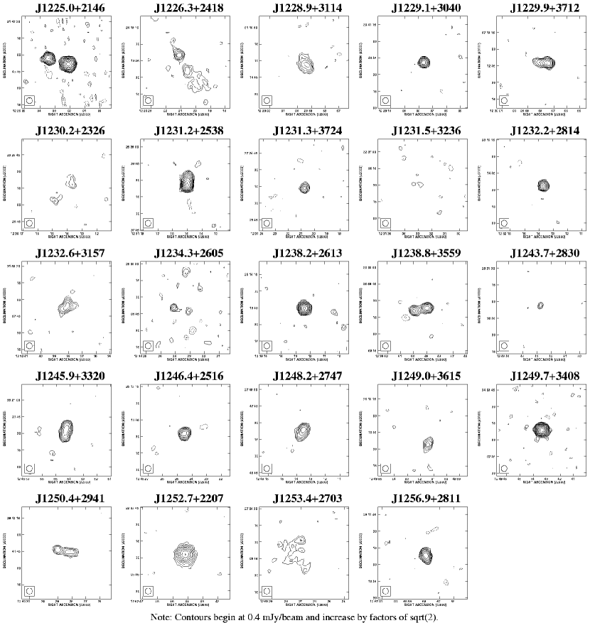
Figure 10: Images from the FIRST survey of the 24 out of 26 ultra-steep spectrum sources identified at 74 MHz, which had NVSS counterparts.

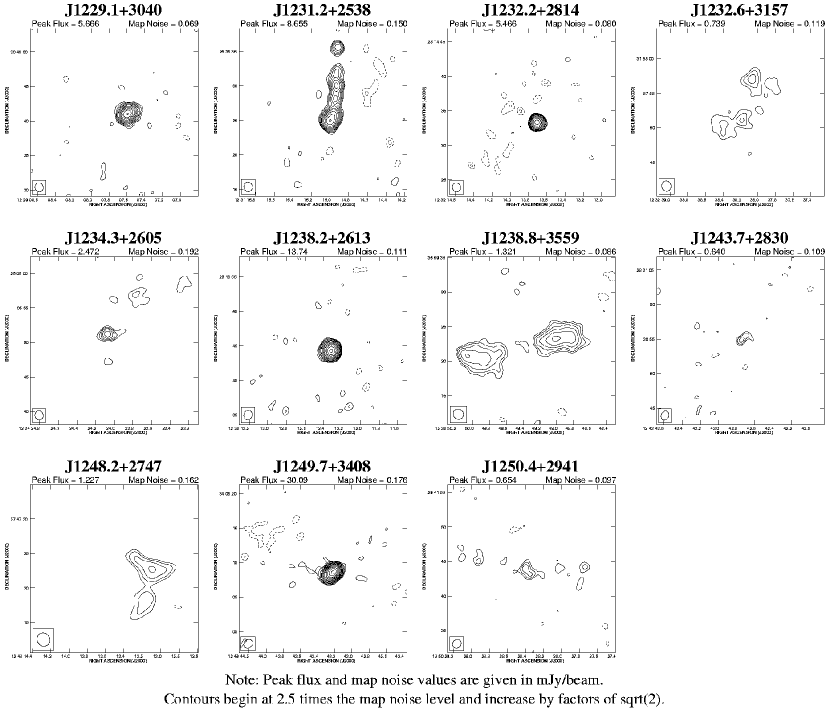
Figure 11: Images of the 11 detections from the 18 USS sources observed with the VLA A-configuration at 1.4 GHz. The remaining 7 are diffuse enough to be resolved out at this resolution of roughly $1.4^{\prime\prime}$.

There are four main possibilities for the identities of such USS sources: (1) pulsars, (2) high redshift radio galaxies (HzRGs: $z>2$), (3) cluster halos or relics (CHRs) and (4) fossil radio galaxies (FRGs: radio galaxies for which the energized particles have undergone significant spectral aging). As this survey is located near the north galactic pole, we expect very few if any pulsars. Using the most recent estimate for the radio luminosity function of CHRs (Enßlin & Röttgering, 2002), we predict that on the order of 1 CHR will be detectable in this region given our sensitivity limit, so this is a real possibility. HzRGs, cluster halos and fossil radio galaxies can be distinguished by their morphologies. We expect small ($\leq 30^{\prime\prime}$) FRII morphologies for HzRGs, while cluster halos or fossil radio galaxies will be much larger and more diffuse. It is difficult to qualify the morphology with the $25^{\prime\prime}$ resolution of our 74 MHz images, so again we turn to the 1.4 GHz FIRST survey (White et al., 1997) with its resolution of $5.4^{\prime\prime}$. In Figure 10 we present FIRST images of each of the 24 USS sources with an NVSS counterpart. Comparison with the POSS-II shows matches or possible matches to 4 out of 24 sources, roughly consistent with the 15% reported by De Breuck et al. (2000). We have also begun our own follow-up observations at 1.4 GHz with the VLA in A-configuration which provides roughly $1.4^{\prime\prime}$ resolution. So far we have so observed 18 of the 24 USS sources with NVSS counterparts and 11 of these were detected (Figure 11), with the remaining 7 likely resolved out. A list of all USS sources we found is provided in the print version of Table 2, and brief descriptions of each USS source follows below.

5.2 Brief Description of Individual USS Sources

The following are brief notes on each USS source. Source images at 1.4 GHz are described from FIRST ($5.4^{\prime\prime}$ resolution) and or VLA A-configuration follow-up ($1.4^{\prime\prime}$ resolution). We speculate on the identity of each source from the four main classes of USS objects: pulsar, cluster halo/relic (CHR), fossil radio galaxy (FRG) or high redshift radio galaxy (HzRG).

J1225.0$+$2146: The FIRST map shows a bright double lobed FRII with a separation of roughly $25^{\prime\prime}$. This is likely to be a HzRG or FRG.

J1226.3$+$2418: The FIRST map shows a $20^{\prime\prime}$ FRII with diffuse extension. A-configuration resolved out this source. It was identified in the POSS-II so it probably isn’t high redshift. This is likely to be a FRG.

J1228.9$+$3114: The FIRST map shows a diffuse blob of about $15^{\prime\prime}$ which is resolved out in A-configuration. This is likely to be a high-$z$ CHR, HzRG or FRG.

J1229.1$+$3040: Unresolved in FIRST but a fit to the A-configuration map shows a source size of about $1^{\prime\prime}$. This is likely a HzRG.

J1229.9$+$3712: Head-tail morphology in FIRST map. This is likely to be a HzRG or FRG.

J1230.2$+$2326: Faint double source in FIRST maps, resolved out in A-configuration. It was identified in the POSS-II so it probably isn’t high redshift. This is likely to be a FRG.

J1230.6$+$3247: No FIRST or NVSS counterpart.

J1231.2$+$2538: A-configuration shows core-jet morphology with an extent of $12^{\prime\prime}$. This is likely to be a HzRG or FRG.

J1231.3$+$3724: Unresolved in FIRST. This is likely to be a pulsar or HzRG.

J1231.5$+$3236: Resolved out in FIRST and A-configuration. This is likely to be a high-$z$ CHR or FRG.

J1232.2$+$2814: Unresolved in FIRST and A-configuration maps. This is likely to be a pulsar or HzRG.

J1232.6$+$3157: A-configuration shows a $7^{\prime\prime}$ FRII with much diffuse emission. This is likely to be a high-$z$ CHR, HzRG or FRG.

J1234.3$+$2605: Unresolved in FIRST but a fit to the A-configuration map shows a source size of about $1^{\prime\prime}$. This is likely a HzRG.

J1238.2$+$2613: Unresolved in FIRST but a fit to the A-configuration map shows a source size of about $0.5^{\prime\prime}$. This is likely a HzRG.

J1238.8$+$3559: FIRST and A-configuration show a well defined $17^{\prime\prime}$ FRII. This is likely to be a HzRG or FRG.

J1243.7$+$2830: FIRST and A-configuration show a faint $2^{\prime\prime}$ elongated object. This is likely to be a HzRG or FRG.

J1245.9$+$3320: FIRST shows a roughly $15^{\prime\prime}$ FRI morphology, which is resolved out in A-configuration. This is likely to be a high-$z$ CHR or FRG.

J1246.4$+$2516: FIRST shows a roughly $10^{\prime\prime}$ blob, which is resolved out in A-configuration. This is likely to be a high-$z$ CHR or FRG.

J1248.2$+$2747: FIRST and A-configuration show a faint $6^{\prime\prime}$ FRII morphology. This is likely to be a HzRG or FRG.

J1249.0$+$3615: FIRST shows a roughly $10^{\prime\prime}$ FRI morphology. This is likely to be a high-$z$ CHR or FRG.

J1249.7$+$3408: Unresolved in FIRST but a fit to the A-configuration map shows a source size of about $0.8^{\prime\prime}$. This is likely a HzRG.

J1250.4$+$2941: FIRST shows a $20^{\prime\prime}$ FRI morphology, which is mostly resolved out in A-configuration. This is likely to be a HzRG or FRG.

J1252.7$+$2207: FIRST shows a $20^{\prime\prime}$ diffuse blob. This is likely to be a high-$z$ CHR, HzRG or FRG.

J1253.4$+$2703: FIRST shows a very diffuse object of about $40^{\prime\prime}$ diameter which is resolved out in A-configuration. This is an ideal CHR candidate, though no nearby clusters are known.

J1253.6$+$2509: No FIRST or NVSS counterpart.

J1256.9$+$2811: FIRST shows a $15^{\prime\prime}$ FRI morphology. This is likely to be a high-$z$ CHR, HzRG or FRG.

6 Conclusions and Future Plans

We have completed a deep, high resolution survey at 74 MHz and identified 949 sources. We measured the differential source counts between roughly 0.22 and 11 Jy, and find them consistent with those found at 327 MHz (Wieringa, 1991) adjusted by a spectral index of roughly $-0.75<\alpha<-0.5$. Comparison with the 1.4 GHz surveys NVSS and FIRST shows that the average source in our survey is steeper than this. This could be explained if a significant fraction of sources become flat or inverted between 327 MHz and 74 MHz, and so are selected against by our flux limited survey. We find that fainter sources tend to have slightly flatter spectra. Source size studies with the FIRST survey indicate that the flat spectrum objects are much smaller than the steeper spectrum objects on average.

A small fraction of sources, 26 out of 949, qualify as USS sources with spectral indices steeper than $\alpha<-1.2$. We present a list of these sources, along with FIRST images of 24 of these and higher resolution A-configuration VLA images of 18 USS sources. We find that all but a few of these are good candidates for high redshift radio galaxies, while the others are probably fossil radio galaxies or cluster halo, relic systems. We plan optical and spectroscopic follow-up on the HzRG candidates to measure their redshifts.

Acknowledgements

We thank W. C. Erickson for providing us with the data used for this survey. The authors made use of the database CATS (Verkhodanov et al., 1997) of the Special Astrophysical Observatory. This research has made use of the NASA/IPAC Extragalactic Database (NED) which is operated by the Jet Propulsion Laboratory, Caltech, under contract with the national aeronautics and spece administration. The Second Palomar Observatory Sky Survey (POSS-II) was made by the California Institute of Technology with funds from the National Science Foundation, the National Geographic Society, the Sloan Foundation, the Samuel Oschin Foundation, and the Eastman Kodak Corporation. ASC acknowledges fellowship support from the National Reseach Council. Basic research in radio astronomy at the NRL is supported by the Office of Naval Research.

Figure 1: The sensivitiy ($5\sigma$) and resolution of our deep 74 MHz radio survey compared to that of the major low frequency radio surveys. The dotted line on the sensitivity plot (top) shows the flux density of a source at our sensitivity limit assuming a spectral index of $\alpha=-0.7$.

Figure 4: (page 1 of 4) Maps of the 80 largest objects detected at 74 MHz. These objects all have a fitted source size (for single sources) or maximum separation between components (for multiple sources) of at least $48.4^{\prime\prime}$.

Figure 4: (page 2 of 4) Maps of the 80 largest objects detected at 74 MHz. These objects all have a fitted source size (for single sources) or maximum separation between components (for multiple sources) of at least $48.4^{\prime\prime}$.

Figure 4: (page 3 of 4) Maps of the 80 largest objects detected at 74 MHz. These objects all have a fitted source size (for single sources) or maximum separation between components (for multiple sources) of at least $48.4^{\prime\prime}$.

Figure 4: (page 4 of 4) Maps of the 80 largest objects detected at 74 MHz. These objects all have a fitted source size (for single sources) or maximum separation between components (for multiple sources) of at least $48.4^{\prime\prime}$.

Figure 5: Euclidean-normalized differential source count. Also plotted are source counts at 327 MHz (Wieringa, 1991) adjusted for various spectral indices.

Figure 6: Spectral indices ($\alpha_{74}^{1400}$) versus 74 MHz integrated flux density. Spectral index upper limits are plotted for the two sources without NVSS detections.

Figure 8: Spectral histogram along with median sources sizes as a function of spectral index. Source sizes are determined with the FIRST images, while spectral indices are determined using the 74 MHz integrated flux density and the NVSS flux densities. Not enough sources were detected with $\alpha_{74}^{1400}<-1.45$ or $\alpha_{74}^{1400}>-0.25$ for meaningful statistics in those regions.

Figure 9: Radio color-color diagram of the 545 out of 949 sources with both an NVSS and a WENSS counterpart. The diagonal line represents the location of sources for which $\alpha_{74}^{325}=\alpha_{325}^{1400}$. For most sources, the spectum flattens considerably in the lower frequency interval.

Table 1: Survey Area

Noise Limit	Area	Source Count
(mJy/beam)	(deg.2)	(number)
25	2.5	23
27	8.6	62
30	22.4	158
35	50.0	356
40	78.2	535
50	119.1	765
60	142.7	873
70	156.9	924
80	165.1	949

Table 2: USS Source List

Source	$\alpha$ (J2000)	$\delta$ (J2000)	$S_{74,int}$	$\alpha_{74}^{1400}$	POSS-II ID
	(h m s)	(∘ ′ ′′)	Jy
J1225.0$+$2146	12 25 02.26	$+$21 46 52.5	2.213	-1.25	N
J1226.3$+$2418	12 26 20.65	$+$24 18 43.6	0.943	-1.36	Y
J1228.9$+$3114	12 28 59.58	$+$31 14 57.6	0.608	-1.36	N
J1229.1$+$3040	12 29 07.75	$+$30 40 41.2	0.356	-1.27	N
J1229.9$+$3712	12 29 58.03	$+$37 12 48.8	0.635	-1.25	N
J1230.2$+$2326	12 30 14.05	$+$23 26 17.2	0.968	-1.63	Y
J1230.6$+$3247	12 30 37.90	$+$32 47 21.9	0.188	$<-1.47$
J1231.2$+$2538	12 31 15.08	$+$25 38 26.3	1.064	-1.20	?
J1231.3$+$3724	12 31 20.77	$+$37 24 17.4	0.477	-1.51	N
J1231.5$+$3236	12 31 32.71	$+$32 36 30.1	0.311	-1.52	N
J1232.2$+$2814	12 32 13.76	$+$28 14 34.9	0.327	-1.36	N
J1232.6$+$3157	12 32 38.23	$+$31 57 52.1	0.359	-1.35	N
J1234.3$+$2605	12 34 23.25	$+$26 05 50.5	0.402	-1.61	N
J1238.2$+$2613	12 38 12.40	$+$26 13 45.8	0.728	-1.30	N
J1238.8$+$3559	12 38 49.30	$+$35 59 22.9	0.634	-1.33	N
J1243.7$+$2830	12 43 42.75	$+$28 30 55.5	0.712	-1.73	N
J1245.9$+$3320	12 45 54.20	$+$33 20 32.1	1.140	-1.40	N
J1246.4$+$2516	12 46 24.49	$+$25 16 35.1	0.347	-1.29	N
J1248.2$+$2747	12 48 13.51	$+$27 47 22.6	0.624	-1.31	N
J1249.0$+$3615	12 49 01.82	$+$36 15 46.8	0.440	-1.20	?
J1249.7$+$3408	12 49 43.34	$+$34 08 09.2	1.383	-1.23	N
J1250.4$+$2941	12 50 28.33	$+$29 41 43.8	0.395	-1.35	N
J1252.7$+$2207	12 52 44.13	$+$22 07 04.9	0.940	-1.22	N
J1253.4$+$2703	12 53 26.85	$+$27 03 50.0	0.838	-1.30	N
J1253.6$+$2509	12 53 39.24	$+$25 09 57.7	0.472	$<-1.78$
J1256.9$+$2811	12 56 58.15	$+$28 11 09.7	0.524	-1.32	N

Note. — The complete catalog is published in its entirety in the electronic edition of the Astrophysical Journal.

References

- Bettoni et al. (2003) Bettoni, D., Falomo, R., Fasano, G., & Govoni, F. 2003, A&A, 399, 869
- Blundell et al. (1998) Blundell K.M., Rawlings S., Eales S.A., Taylor G., Bradley A.D., 1998, MNRAS, 295, 265
- Blundell, Rawlings, & Willott (1999) Blundell, K. M., Rawlings, S., & Willott, C. J. 1999, AJ, 117, 677
- Carilli et al. (1997) Carilli, C. L., Roettgering, H. J. A., van Ojik, R., Miley, G. K., & van Breugel, W. J. M. 1997, ApJS, 109, 1
- Chambers et al. (1996) Chambers, K. C., Miley, G. K., van Breugel, W. J. M., & Huang, J.-S. 1996, ApJS, 106, 215
- Condon et al. (1998) Condon, J. J., Cotton, W. D., Greisen, E. W., Yin, Q. F., Perley, R. A., Taylor, G. B., & Broderick, J. J. 1998, AJ, 115, 1693
- Cornwell & Perley (1992) Cornwell, T. J. & Perley, R. A. 1992, A&A, 261, 353
- Cotton & Condon (2002) Cotton, W. D. & Condon, J. J. 2002, URSI General Assemply, 17-24 August, 2002, Maastricht, The Netherlands, paper 0944, pp 1-4.
- Cuby et al. (2003) Cuby, J.-G., Le Fèvre, O., McCracken, H., Cuillandre, J.-C., Magnier, E., & Meneux, B. 2003, A&A, 405, L19
- De Breuck et al. (2000) De Breuck, C., van Breugel, W., Röttgering, H. J. A., & Miley, G. 2000, A&AS, 143, 303
- De Breuck et al. (2002) De Breuck, C., van Breugel, W., Stanford, S. A., Röttgering, H., Miley, G., & Stern, D. 2002, AJ, 123, 637
- Dunlop et al. (2003) Dunlop, J. S., McLure, R. J., Kukula, M. J., Baum, S. A., O’Dea, C. P., & Hughes, D. H. 2003, MNRAS, 340, 1095
- Enßlin & Röttgering (2002) Enßlin, T. A. & Röttgering, H. 2002, A&A, 396, 83
- Gower, Scott, & Wills (1967) Gower, J. F. R., Scott, P. F., & Wills, D. 1967, MmRAS, 71, 49
- Hu et al. (2002) Hu, E. M., Cowie, L. L., McMahon, R. G., Capak, P., Iwamuro, F., Kneib, J.-P., Maihara, T., & Motohara, K. 2002, ApJ, 568, L75
- Jarvis et al. (2001) Jarvis, M. J., Rawlings, S., Eales, S., Blundell, K. M., Bunker, A. J., Croft, S., McLure, R. J., & Willott, C. J. 2001, MNRAS, 326, 1585
- Kassim et al. (1993) Kassim, N. E., Perley, R. A., Erickson, W. C., & Dwarakanath, K. S. 1993, AJ, 106, 2218
- Kassim et al. (2000) Kassim, N. E., Lazio, T. J. W., Erickson, W. C., Crane, P. C., Perley, R. A., & Hicks, B. 2000, Proc. SPIE, 4015, 328
- Kassim et al. (2003) Kassim, N. E., Lazio, T. J. W., Erickson, W. C., Perley, R. A., Cotton, W. D., Greisen, E. W, Hicks, B., Cohen, A. S., Lane, W. M., & Rickard, L. J. 2003,“The 74 MHz System on the Very Large Array”, (in prep)
- Kodaira et al. (2003) Kodaira, K. et al. 2003, PASJ, 55, L17
- Magorrian et al. (1998) Magorrian, J. et al. 1998, AJ, 115, 2285
- Overzier et al. (2003) Overzier, R. A., Röttgering, H. J. A., Rengelink, R. B., & Wilman, R. J. 2003, A&A, 405, 53
- Pilkington & Scott (1965) Pilkington, J. D. H. & Scott, P. F. 1965, MmRAS, 69, 183
- Rawlings et al. (1996) Rawlings, S., Lacy, M., Blundell, K. M., Eales, S. A., Bunker, A. J., & Garrington, S. T. 1996, Nature, 383, 502
- Rengelink et al. (1997) Rengelink, R. B., Tang, Y., de Bruyn, A. G., Miley, G. K., Bremer, M. N., Roettgering, H. J. A., & Bremer, M. A. R. 1997, A&AS, 124, 259
- Röttgering et al. (1994) Röttgering H. J. A., Lacy M., Miley G. K., Chambers K. C., Saunders R., 1994, A&AS, 108, 79
- Steidel et al. (1996) Steidel, C. C., Giavalisco, M., Pettini, M., Dickinson, M., & Adelberger, K. L. 1996, ApJ, 462, L17
- Steidel et al. (1999) Steidel, C. C., Adelberger, K. L., Giavalisco, M., Dickinson, M., & Pettini, M. 1999, ApJ, 519, 1
- van Breugel et al. (1999) van Breugel, W., De Breuck, C., Stanford, S. A., Stern, D., Röttgering, H., & Miley, G. 1999, ApJ, 518, L61
- Verkhodanov et al. (1997) Verkhodanov, O. V., Trushkin, S. A., Andernach, H., & Chernenkov, V. N. 1997, ASP Conf. Ser. 125: Astronomical Data Analysis Software and Systems VI, 6, 322
- Wall & Jackson (1997) Wall, J. V., & Jackson, C. A. 1997, MNRAS, 290, L17
- White et al. (1997) White, R. L., Becker, R. H., Helfand, D. J., & Gregg, M. D. 1997, ApJ, 475, 479
- Wieringa (1991) Wieringa, M. H. 1991, Ph.D. Thesis, Leiden University
- Willott et al. (2003) Willott, C. J., Rawlings, S., Jarvis, M. J., & Blundell, K. M. 2003, MNRAS, 339, 173