From the production of primordial perturbations to the end of inflation

Abstract

In addition to generating the appropriate perturbation power spectrum, an inflationary scenario must take into account the need for inflation to end subsequently. In the context of single-field inflation models where inflation ends by breaking of the slow-roll condition, we constrain the first and second derivatives of the inflaton potential using this additional requirement. We compare this with current observational constraints from the primordial spectrum and discuss several issues relating to our results.

I Introduction

With the increasing precision of cosmological observations, inflation has become the favored candidate for explaining the origin of perturbations in the Universe infrev . While some plausible scenarios have recently been introduced whereby adiabatic perturbations are generated after inflation from isocurvature perturbations laid down during inflation isoad , the generation of adiabatic density perturbations during inflation remains the simplest one. However, although inflationary models give an excellent fit to most recent data including that of the Wilkinson Microwave Anisotropy Probe (wmap) wmap ; Petal , the perturbations are observable only over a fairly narrow range of scales, corresponding to about four orders of magnitude in wavenumber, thus allowing us to constrain only a small segment of the inflationary potential. Nevertheless, there is one further piece of information that can be brought into play infend , which is that we know that inflation must come to an end soon after the observable perturbations are generated.

The literature describes three ways in which inflation might end. In the simplest scenario, requiring just a single scalar field, the logarithm of the potential driving inflation becomes too steep to sustain inflation, leading to the end of the slow-roll regime and usually giving way to a series of oscillations about a minimum in the potential. A second popular possibility is an instability, associated with a second scalar field, which removes the potential energy driving inflation; this is the key idea of the hybrid inflation paradigm hyb , where inflation ends by a phase transition. Much less discussed is a third possibility, that at some energy scale the underlying equations of motion are modified, an example being the steep inflation model steep where inflation is sustained only by corrections to the Friedman equation at high energies in a braneworld model, with inflation ending as the energy scale drops and these corrections become unimportant.

In the hybrid inflation case, the inflaton field is normally unaware of the existence of the instability until its onset, and the inflaton dynamics gives no clue as to when it might happen. In that case, we can expect no useful extra information from the need to end inflation. If the underlying equations can be modified, as in the steep inflation case, there are many ways in which this could happen and it is unlikely that any useful model-independent statements can be made. In this paper, we therefore restrict our attention to models with a single scalar field, in which inflation ends by breaking of the slow-roll condition. Our aim is to assess whether the requirement to end inflation imposes useful additional constraints on the inflaton potential, and to discover whether there are regions of parameter space permitted by the perturbation data which are ill-suited to a satisfactory end to inflation in this manner.

It was recently shown that there is a firm upper limit $N_{\mathrm{max}}$ to the number of $e$-foldings $N_{\mathrm{inf}}$ before the end of inflation at which observable perturbations were generated Ninf . In this work, we aim to use the value of $N_{\mathrm{max}}$ to set some conservative constraints on the first two derivatives of the inflaton potential in the context of single-field inflation, which can be compared to the region permitted by the observed perturbations. In other words we want to look at the generic predictions of single-field inflation by defining a region in the primordial power spectrum parameter space compatible with the paradigm. This goal is similar to that of analyses using the inflationary flow equations flow , such as Peiris et al. Petal and Kinney et al. KKMR which are based on the method of Easther and Kinney EK , but as we will discuss our approach is different in its physical content and makes more restrictive assumptions about the shape of the potential.

The paper is organized as follows: Section II is devoted to stating our assumptions and explaining our methodology, Section III gives the results and analysis, and Section IV is a general discussion on related issues. We assume $m_{\mathrm{Pl}}=1$ throughout.

II Methodology

In this section we explain how we constrain the inflaton potential in the context of single-field inflation. The main idea is to test whether it is possible to build a reasonable model which takes into account the upper limit on the number of $e$-foldings $N_{\mathrm{inf}}$ before the end of inflation, given the shape of the potential in the range probed by observations.

Given an inflationary potential $V(\phi)$ and an initial value of the field $\phi_{*}$ (corresponding to the horizon crossing of a pivot scale $k_{*}$) we can compute a Taylor expansion of $V(\phi)$ around $\phi_{*}$. In the context of slow-roll and in the face of the current observational data, one does not expect more than the first two or three derivatives to play an important role in the range of scales probed by cmb observations and galaxy distribution surveys. Before going into more details, it is useful to note that the evolution of the field as a function of the number of $e$-foldings does not depend on the normalization of the potential. Therefore, throughout the paper we use the parameters $V^{\prime}/V$, $V^{\prime\prime}/V$, $V^{\prime\prime\prime}/V$, etc. which are evaluated at $\phi_{*}$. Also, by convention we take the first derivative to be negative.

Now, let us introduce the set of slow-roll parameters STEG ; LLMS

$$\varepsilon_{0} = \frac{H(0)}{H(N)}\,\mathrm{,}$$ (1)

$$\varepsilon_{n+1} = \frac{\mathrm{d}\ln\left|\varepsilon_{n}\right|}{\mathrm{d}N}\qquad\mathrm{for}\quad n\geq 0\,\mathrm{,}$$ (2)

where $H$ is the Hubble parameter and $N$ is the number of $e$-foldings since the crossing of the horizon by the pivot scale $k_{*}$. This particular choice of definition is known as the horizon-flow parameters. We can compute (to first-order) $V^{\prime}/V$ and $V^{\prime\prime}/V$ as functions of $\varepsilon_{1}$ and $\varepsilon_{2}$

$$\frac{V^{\prime}}{V} \simeq -4\sqrt{\pi\varepsilon_{1}}\,\mathrm{,}$$ (3)

$$\frac{V^{\prime\prime}}{V} \simeq 4\pi(4\varepsilon_{1}-\varepsilon_{2})\,\mathrm{,}$$ (4)

which relates the shape of the potential with the inflationary dynamics. Conversely, we can recover the slow-roll parameters from the derivatives of the potential

$$\varepsilon_{1} \simeq \frac{1}{16\pi}\left(\frac{V^{\prime}}{V}\right)^{2}\,\mathrm{,}$$ (5)

$$\varepsilon_{2} \simeq \frac{1}{4\pi}\left[\left(\frac{V^{\prime}}{V}\right)^{2}-\frac{V^{\prime\prime}}{V}\right]\,\mathrm{.}$$ (6)

These slow-roll parameters can then be related to primordial power spectrum parameters such as the scalar and tensor spectral indices $n_{\mathrm{S}}-1\simeq-2\varepsilon_{1}-\varepsilon_{2}$ and $n_{\mathrm{T}}\simeq-2\varepsilon_{1}$, the tensor to scalar ratio $R\simeq 16\varepsilon_{1}$, etc. Therefore, we will interchangeably use any independent pair of these parameters. Note that since the constraint on the running $\alpha_{\mathrm{S}}\simeq-2\varepsilon_{1}\varepsilon_{2}-\varepsilon_{2}\varepsilon_{3}$ is too weak at the moment (see Ref. LL03 for comments on this issue), we will assume some theoretical prior on this parameter. It is important to stress that in this work we do not want to constrain higher derivatives; rather, we are trying to find a region of the $V^{\prime}/V$–$V^{\prime\prime}/V$ space that is compatible with a large class of single-field inflation models.

Now, as explained above, our aim is to try to build a working single-field inflation model (i.e. an inflaton potential) by expanding the potential as a Taylor series, fixing the first two derivatives to reasonable values, and then varying the higher-order derivatives using a random process. We set the following rules to define a working model:

1. The shape of the potential should be consistent with the constraints on the primordial perturbation power spectrum, as well as with the prior on the running $\alpha_{\mathrm{S}}$.

2. The potential should either be convex ($V^{\prime\prime}/V>0$) throughout the evolution (large-field inflation) or at first concave ($V^{\prime\prime}/V<0$) and eventually convex (small-field inflation).

3. The number of $e$-foldings between the time the scale $k_{*}$ leaves the horizon and the end of inflation ($\varepsilon_{1}=1$) should be less than $N_{\mathrm{max}}$.

Concerning the first rule, we look at a region of the parameter space $V^{\prime}/V$–$V^{\prime\prime}/V$ approximately consistent with observations of $n_{\mathrm{S}}-1$ and $R$ — we will later contrast our results with actual constraints from wmap and 2df. We initially impose the theoretical prior $-0.04<\alpha_{\mathrm{S}}<0.02$. In anticipation that future observations will pin down the running more precisely, we then go on to examine successively the following subcases: (i) $-0.04<\alpha_{\mathrm{S}}<-0.02$, (ii) $-0.02<\alpha_{\mathrm{S}}<0$, and (iii) $0<\alpha_{\mathrm{S}}<0.02$, so as to investigate how future constraints may affect the overall picture. As

$$\begin{split}\frac{V^{\prime\prime\prime}}{V}&\simeq\sqrt{\frac{\pi}{\varepsilon_{1}}}\left(-24\varepsilon_{1}^{2}+18\varepsilon_{1}\varepsilon_{2}-3\varepsilon_{2}\varepsilon_{3}\right)\\ &\simeq\sqrt{\frac{\pi}{\varepsilon_{1}}}\left(-24(\varepsilon_{1}^{2}-\varepsilon_{1}\varepsilon_{2})+3\alpha_{\mathrm{S}}\right)\,\mathrm{,}\end{split}$$ (7)

these constraints on the running impose constraints on the third derivative of the potential. Then, we assume that higher derivatives are negligible in the range of values of the field corresponding to observed scales. Specifically, we impose

$$\left|\frac{1}{4!}\frac{V^{(4)}}{V}\Delta\phi^{4}\right|<\left|\frac{1}{3!}\frac{V^{\prime\prime\prime}}{V}\Delta\phi^{3}\right|\,\mathrm{,}$$ (8)

where $\Delta\phi$ is the distance run by the field when producing the observed perturbations (corresponding to roughly 7 $e$-foldings, 3.5 on each side of $\phi_{*}$). This means that the fourth-order term in the Taylor expansion is assumed not to overtake the third-order term until the field runs about twice the distance to the edge of the observed region. Note that as a result, the fourth derivative term cannot contribute significantly to the curvature of the potential inside the observed region. In addition, in order to find working models more easily, we use the practical recipe

$$\left|\frac{1}{5!}\frac{V^{(5)}}{V}\Delta\phi_{3,4}^{5}\right|<\left|\frac{1}{4!}\frac{V^{(4)}}{V}\Delta\phi_{3,4}^{4}\right|\,\mathrm{,}$$ (9)

where $\Delta\phi_{3,4}$ is the value of the field for which the fourth order term equals the third order term in the Taylor expansion. Note that if $V^{\prime}/V$ and $V^{\prime\prime}/V$ are fixed, the uncertainty on $\alpha_{\mathrm{S}}$ still allows $V^{\prime\prime\prime}/V$ to vary and therefore the possibility of having $V^{\prime\prime\prime}/V\simeq 0$ (and hence Eqs. (8) and (9) being too strong constraints) is avoided.

The second rule is assumed in order to maintain the simplicity of the model, as this is the main reason for considering single-field inflation. Also, most models in the literature are of this form. We consider Taylor expansions of third, fourth and fifth order. It is important to note that our class of models is broader than a set of polynomial potentials, since the expansion need only approximate the true potential over a limited range, with the order of the expansion reflecting the number of degrees of freedom we have to shape the potential in order to fulfil our set of rules. We checked that a fifth degree polynomial can fit a wide range of potentials from $\phi_{*}$ to the value of the field corresponding to the end of inflation.

We also investigated the effect of imposing the constraint that $V=0$ at the minimum of the potential. However we found that this condition complicates the analysis without adding anything useful, since after inflation ends it is usually not hard for the potential to then shape itself to form a satisfactory minimum. In any case it is not our intention to address the post-inflationary dynamics.

Finally, concerning the third rule, inflation must end by breaking of the slow-roll condition ($\varepsilon_{1}=1$) and this should happen within a certain number of $e$-foldings $N_{\mathrm{inf}}<N_{\mathrm{max}}$ after the scale $k_{*}$ crosses the horizon. The uncertainty on $N_{\mathrm{inf}}$ comes mainly from the reheating process, which can be very brief or alternatively can last until nucleosynthesis. Assuming instantaneous reheating and with $h\simeq 0.72$, $\Omega_{\mathrm{m}}\simeq 0.27$, the amplitude of scalar perturbations $A_{\mathrm{S}}\simeq 2.3\times 10^{-9}$ and the pivot scale $k_{*}\simeq 0.01$Mpc^-1 (see Ref. LL03 ) we have

$$N_{\mathrm{max}} \simeq 60+\frac{1}{4}\ln(\epsilon_{1})-\frac{1}{4}\ln(\mathcal{D})\,\mathrm{,}$$ (10)

where $\mathcal{D}$ is the drop in the energy density between the time the scale $k_{*}$ crosses the horizon and the time inflation ends. The discrepancy between this equation and the results given in Ref. Ninf comes from choosing a different scale as a starting point.

Our procedure is as follows: We fix the pair $V^{\prime}/V$ and $V^{\prime\prime}/V$, randomly choose the higher derivatives, and then test the resulting potential against our set of rules. We repeat this step until we find a working model. If we cannot build a potential fulfilling the three rules stated above after a certain number of tries $n_{\mathrm{tries}}$, then we say that this pair of parameters is not consistent with single-field inflation, and move onto the next values of $V^{\prime}/V$ and $V^{\prime\prime}/V$. We took $n_{\mathrm{tries}}=300^{\nu}$, where $\nu$ is the number of degrees of freedom describing the potential after the first two derivatives have been chosen (i.e. $\nu=1$, $2$ or $3$), and tested other values to ensure that our results do not depend on this choice.

III Results

Figure 1: Boundaries between the regions where it is possible to build a working model (shaded) and regions where single-field inflation is excluded. We assume $-0.04<\alpha_{\mathrm{S}}<0.02$. The black line at $V^{\prime\prime}=0$ separates small-field and large-field models, and the dashed line shows $\varepsilon_{2}=0$. The other lines show the different orders in the expansion of the potential, with the labels always placed outside the allowed region. The dots show models from the Monte-Carlo Markov chain fitting the perturbation data.

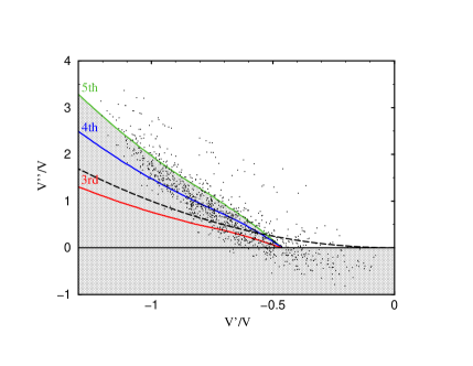
In this section we present our results as boundaries between allowed and excluded regions in the $V^{\prime}/V$–$V^{\prime\prime}/V$ space and in the $(n_{\mathrm{S}}-1)$–$R$ space. In other words, we are seeking to make some falsifiable predictions for our class of single-field inflation models.

Figure 2: Same as Fig. 1 but with more restrictive assumptions on the running: (i) $-0.04<\alpha_{\mathrm{S}}<-0.02$, (ii) $-0.02<\alpha_{\mathrm{S}}<0$ and (iii) $0<\alpha_{\mathrm{S}}<0.02$.

The main result is displayed in Fig. 1, for which we assume $-0.04<\alpha_{\mathrm{S}}<0.02$. For each order in the expansion of the potential there is a line which represents the boundary between the region where it is possible to build a working model (shaded) and the region where single-field inflation is excluded. The dots are independent samples from the Monte-Carlo Markov chain used in Ref. LL03 to fit wmap and 2df, and thus represent models providing a good fit to the perturbation data. We also plot the line $\varepsilon_{2}=0$ to compare with the naive expectation that only models with $\epsilon_{2}>0$ are suitable candidates for violating slow-roll (since by definition $\mathrm{d}\varepsilon_{1}/\mathrm{d}N=\varepsilon_{1}\varepsilon_{2}$).

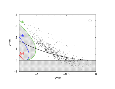
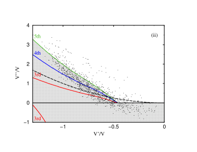
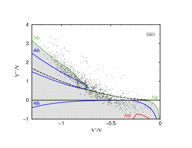
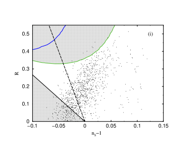
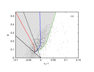
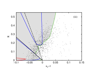
In Fig. 2 we make more restrictive assumptions on the running, with the three graphs showing the cases (i), (ii) and (iii) as described in Section II. Figure 3 shows the same information but displayed in the space of observable parameters, that is $n_{\mathrm{S}}-1$ and $R$. We comment on small-field and large-field inflation separately.

III.1 Small-field inflation

First, let us consider potentials with a negative second derivative $V^{\prime\prime}<0$, which are found in the lower part of each of the panels in Fig. 1 and Fig. 2, and at the left lower corner of the panels in Fig. 3. We can see in Fig. 1 that these models are currently not constrained by the upper bound $N_{\mathrm{max}}$. Indeed, it is always possible to build a working model even when considering only a third-order expansion. This is because as long as its slope is not bounded outside the region probed by observations, nothing prevents the potential from steepening enough in order to violate slow-roll before the number of $e$-foldings reaches $N_{\mathrm{max}}$.

Even when tightening our assumptions on the running (see Fig. 2), models which fit the perturbation data remain almost unconstrained as long as the running is negative. However if the running is positive, panel (iii), the third derivative prevents inflation from ending in time, and unless we use at least a fourth-order expansion, it is difficult to build a working model consistent with observations. Nevertheless, it is fair to say that so far small-field inflation is consistent with observations even when taking into account the constraint on $N_{\mathrm{max}}$.

III.2 Large-field inflation

Figure 3: Same as Fig. 2 but in the $(n_{\mathrm{S}}-1)$–$R$ plane.

In the case of potentials with a positive curvature, the situation is very different. The modulus of the slope of the potential is bounded from above (because of the second rule) and the quickest, and therefore somewhat unrealistic, way to end inflation would be for the potential to become a linear potential as soon as the field leaves the observable region. We studied this kind of potential but it did not lead to any interesting constraint. Now, it is clear that the more derivatives we take into account, the more degrees of freedom we have available to shape the potential into a linear-like potential, and the extra degrees of freedom can conspire to build an extreme model in order to end inflation as quickly as possible. If such a model does not end inflation in time for given values of $V^{\prime}/V$ and $V^{\prime\prime}/V$, then we can be sure that this pair of parameters is inconsistent with our class of single-field inflation models. Note that the allowed models lying close to the fifth-order boundary already require a certain amount of fine tuning between the different derivatives. One could of course expand the potential to sixth-order, but the resulting enlargement of the allowed region would be due to potentials that are even more linear-like and fine-tuned.

Figure 1 shows that a significant fraction (around 30%) of large-field models which fit the wmap and 2df data sets are excluded by the need to end inflation in time. This proportion increases even more (to around 60%) when considering only fourth-order expansion potentials and in the third-order case almost all of them (around 90%) are excluded. It is somewhat unfortunate that the constraints coming from observations and from the need to end inflation lie in the same direction, but it is fair to say that large-field inflation models are under pressure.

This becomes clearer when we consider tighter constraints on the running. We can see in Fig. 2 that a large negative running ($\alpha_{\mathrm{S}}<-0.02$, panel (i)) is almost inconsistent with large-field inflation. This can be easily understood by looking at Eq. (7); rule 2 plays a major role by preventing the curvature of the potential from changing sign, and it will be difficult to build a working model unless $\varepsilon_{1}$ is large ($V^{\prime}/V$ very negative). In the case of a positive running the possibility of a third-order working model is excluded and fourth-order models are difficult to achieve.

On the other hand, panel (ii) in Fig. 2 ($-0.02<\alpha_{\mathrm{S}}<0$) is exactly the same as Fig. 1. This means that it is much easier to end inflation if the running is between $-0.02$ and $0$ than if it is positive or more negative. In other words, for large-field inflation models, the running is tightly constrained by the need to end inflation. As a result, forthcoming surveys may rule out this class of inflation models.

From an observational point of view, when looking at Fig. 3 we see that our conditions clearly favor models with $n_{\mathrm{S}}<1$, and in particular we find that even $n_{\mathrm{S}}=1$ is hard to achieve unless $R$ is large.

IV Discussion

We have been motivated by the flow-equation formalism of Easther and Kinney EK to study the idea of randomly generating a large class of slow-roll inflation models in order to make a comparison with the increasingly restrictive observational constraints. However, as explained in Ref. L03 , the flow equation formalism does not incorporate the underlying inflationary physics via the Euler-Lagrange equation. In our procedure this has been essential since we wanted to place a constraint on the qualitative shape of the inflation potential (via our rule 2).

Nevertheless, it is worth comparing with the results of Refs. Petal ; KKMR which used the flow-equation formalism. First of all, both of those papers have included the running as a parameter when generating their observational constraints. As a result, the observationally favored region in the $(n_{\mathrm{S}}-1)$–$R$ plane is enlarged, giving the effect that the flow-equation formalism currently picks out a small preferred region. Compared with observational constraints with no running, the flow-equation formalism actually generates a large class of models covering almost all of the observably favored region. Our method has generated a more restricted ensemble of inflation models, and from this perspective it can be considered a small step forward. Moreover, we have not tried to display any distribution of models, but instead just defined regions compatible with our class of single-field inflation models, arguing that the models near the edges of these regions are in some sense already fine tuned. This presentation has also allowed us to clarify the effect of adding further derivatives to our expansion of the potential.

Broadly speaking, we found it very easy to construct working models with $V^{\prime\prime}/V<0$, whereas for models with $V^{\prime\prime}/V>0$ the situation is more complex. Specifically, we showed that a lower limit on the amplitude of the slope of the potential does persist in the region classified as large-field inflation, analogous to the lower limit recently used to put pressure on the $\phi^{\alpha}$ inflation models LL03 . This means that the upper limit on $N_{\mathrm{inf}}$ does exert some pressure on inflation model building efforts. In addition, we showed that our constraints have a strong dependence on the running of the spectral index as it determines the value of the third derivative. From an observational point of view, we found that single-field inflation models can give $n_{\mathrm{S}}>1$, but only with a large value of $R$, which is expected to be constrained by upcoming observations.

To summarize, while small-field models are poorly constrained by the maximum number of $e$-foldings, we can see a certain tension against our large-field models and forthcoming observations may actually rule them out. Obviously some fundamental theory could be responsible for a potential with an unexpected shape, but for studying phenomenological models our assumptions seem reasonable. Finally we must stress that $N_{\mathrm{max}}$ is an upper bound and knowing details about the reheating process may lower that bound and lead to even more constraining results.