The evolution of the C/O ratio in metal-poor halo stars

We report new measurements of carbon and oxygen abundances in 34 F and G dwarf and subgiant stars belonging to the halo population and spanning a range of metallicity from [Fe/H] $=-0.7$ to $-3.2$ . The survey is based on observations of four permitted lines of C i near 9100 Å and the O i $\lambda 7774$ triplet, all recorded at high signal-to-noise ratios with the UVES echelle spectrograph on the ESO VLT. The line equivalent widths were analysed with the 1D, LTE, MARCS model atmosphere code to deduce C and O abundances; corrections due to non-LTE and 3D effects are discussed. When combined with similar published data for disk stars, our results confirm the metallicity dependence of the C/O ratio known from previous stellar and interstellar studies: C/O drops by a factor of $\sim 3-4$ as O/H decreases from solar to $\sim 1/10$ solar. Analysed within the context of standard models for the chemical evolution of the solar vicinity, this drop results from the metallicity dependence of the C yields from massive stars with mass loss, augmented by the delayed release of C from stars of low and intermediate mass. The former is, however, always the dominant factor. Our survey has also uncovered tentative evidence to suggest that, as the oxygen abundance decreases below [O/H] $=-1$, [C/O] may not remain constant at [C/O] $=-0.5$, as previously thought, but increase again, possibly approaching near-solar values at the lowest metallicities ([O/H] $\lower 2.15277pt\hbox{$\;\buildrel<\over{\sim}\;$}-3$). With the current dataset this is no more than a $3\sigma$ effect and it may be due to metallicity-dependent non-LTE corrections to the [C/O] ratio which have not been taken into account. However, its potential importance as a window on the nucleosynthesis by Population III stars is a strong incentive for future work, both observational and theoretical, to verify its reality.

1 Introduction

Since Eggen, Lynden-Bell, & Sandage (eggen62 (1962)) showed that it is possible to study the formation history of the Galaxy using stellar abundances, such studies have become an integral part of our understanding of how galaxies evolve. During the Galaxy’s evolution, nucleosynthesis by successive generations of stars proceeded along with dynamical processes. A fossil record of the state of the Galaxy at various epochs in its past is preserved in stars surviving from earlier times to the present; their chemical composition plays an important role in identifying different stages in the formation of the Milky Way (Freeman & Bland-Hawthorn 2002). Furthermore, the relative abundances of pairs of elements—examined as a function of metallicity—can provide clues to the main channels for their nucleosynthesis.

Prime examples are carbon and oxygen, the two most abundant elements after hydrogen and helium and the first to be produced (after He) in the chain of stellar nucleosynthesis which enriched the universe from its primordial mix of light elements to its composition today. The current thinking is that oxygen is synthesised in massive stars and dispersed into the interstellar medium (ISM) by Type II supernovae. Carbon, on the other hand, is produced during helium burning in stars of all masses, but the dependence of its yield on stellar mass and initial composition is not well known.

Clues are provided by the behaviour of C/O vs. O/H. Measurements of carbon and oxygen abundances in Galactic stars (Nissen & Edvardsson 1992; Andersson & Edvardsson andersson94 (1994); Gustafsson et al. gustafsson99 (1999)) and H ii regions in spiral and irregular galaxies (reviewed by Garnett 2003) show a decrease in C/O by a factor of about three as the oxygen abundance decreases from solar to [O/H] $\simeq-1$. This has been interpreted as resulting from the combination of the metallicity dependence of the C yield from the winds of massive stars on the one hand, and the time delay in the release of C from intermediate and low mass stars relative to the prompt enrichment of O from Type II supernovae on the other (Henry, Edmunds, & Köppen 2000; Goswami & Prantzos 2000; Carigi 2000; Chiappini, Romano, & Matteucci 2003b).

The measurements of carbon and oxygen abundances in disk stars cited above used the forbidden [C i] $\lambda 8727.13$ and [O i] $\lambda 6300.30$ lines. However, in halo main sequence stars with [Fe/H] $<-1$ these lines become too weak to be measured reliably. Tomkin et al. (1992) showed that this low metallicity regime can be probed with four stronger high excitation C i lines near 9100 Å together with the oxygen triplet at $\lambda\lambda 7771.94$, 7774.17, 7775.39 . The results of Tomkin et al. hint at interesting features in the behaviour of the [C/O] ratio at low oxygen abundances, but the sample was small because of the practical difficulties of conducting high precision spectroscopy in the far red with the instrumentation available ten years ago. With the advent of large telescopes, equipped with efficient echelle spectrographs and modern detectors, the time is now ripe to re-examine the abundances of carbon and oxygen over the full range of metallicities spanned by Galactic halo stars. We address this topic in the present paper with new observations of 34 halo stars obtained with the Ultraviolet and Visual Echelle Spectrograph (UVES; Dekker et al. 2000) on the European Southern Observatory Very Large Telescope (VLT). The paper is arranged as follows. In Section 2 we give a brief description of the observations and data reduction. The properties of the 34 stars that make up our sample are summarised in Section 3, while Section 4 presents the derivation of the abundances of C and O, together with an assessment of the likely errors. In Section 5 we discuss our findings in the context of chemical evolution models of the solar vicinity. Finally we summarise our main results and conclusions in Section 6.

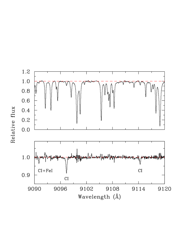
Figure 1: The spectrum of CD$-35\degr 14849$, before (top) and after (bottom) division by the spectrum of a B-type star. The only remnant of the telluric water vapour lines which mar this region of the optical spectrum is a higher level of noise at the wavelengths of the H₂O lines.

2 Observations and data reduction

Our sample consists of 34 F and G-type stars close to the main sequence turn-off in the HR diagram. The stars, all with halo kinematics, were selected mostly from the Strömgren photometric catalogue of Schuster & Nissen (schuster88 (1988)) supplemented with a few very metal-poor stars from Ryan, Norris, & Beers (ryan99 (1999)). The selection criteria were: $5600<\mbox{$T_{\rm eff}$}<6500$ K, $3.7<\mbox{{\rm log}\,$g$}<4.4$, and a smooth distribution of metallicities from [Fe/H] = $-3.2$ to $-0.7$. The stellar visual magnitudes are between $V=7.2$ and 11.5 .

High resolution and signal-to-noise (S/N) spectra of the 34 stars were recorded with UVES in service mode between March and June 2001. The total integration time was typically one hour per star, divided between three 20 minute exposures to facilitate the identification and removal of pixels affected by cosmic-ray events. We used image slicer #1, which gives a resolving power $R\simeq 60\,000$, together with the DIC2 dichroic which divides the spectrum into the blue and red arms with central wavelengths of 4370 Å and 8600 Å respectively. All the C i ($\lambda\lambda 9061.44,9078.29$ and $\lambda\lambda 9094.83,9111.81$) and O i ($\lambda\lambda 7771.94,7774.17,7775.39$) lines of interest fall in the red portion of the spectrum.

Figure 2: Sample portions of the UVES spectra, showing the C i $\lambda 9094.83$ line (left) and the O i $\lambda\lambda 7771.94,7774.17,7775.39$ triplet (right) in three stars with the metallicities indicated. Arrows in the left-hand panels indicate where telluric water vapour lines were divided out. Note that in the star with the lowest metallicity in the present sample, G64–12, the C i and O i lines can still be easily detected at [Fe/H] $=-3.17$ .

The spectra were reduced with the standard echelle data reduction package in IRAF, following the usual steps of bias and scattered light subtraction, flat-fielding, order definition, wavelength calibration (by reference to the emission lines spectrum of the internal Th-Ar lamp) and cosmic ray rejection (by comparing the three individual exposures of each star). The far red portion of the optical spectrum where the C i lines are located is affected by the presence of several, strong, telluric water vapour lines. They can, however, be removed effectively by division by the spectrum of a hot star (usually of B spectral type), as shown in Figure 1. This process also served to remove any residual fringing which remained after flat-fielding. At the shorter wavelengths of the O i triplet telluric absorption is not a problem, but the spectra of B stars show some intrinsic absorption lines and could therefore not be used to remove the residual fringing. This was accomplished by fitting a high-order spline function to the spectra; with an amplitude of only a few percent and a period of $\sim 2$ Å, the fringing can be distinguished from the narrower stellar absorption lines. The final step in the data reduction consisted of correcting for the stellar radial velocities. Representative portions of the spectra are reproduced in Figure 2. The typical signal-to-noise ratios per pixel near the spectral features of interest are S/N $=200-300$, measured from the rms deviations from the continuum level.

Equivalent widths ($W_{\lambda}$) of the C i and O i lines were measured by direct integration. We can estimate the errors in these values empirically, by comparing (a) two independent spectra available for nine stars which were observed twice for operational reasons, and (b) the equivalent widths of the O i triplet lines which are recorded in two adjacent echelle orders (orders 13 and 14). The first comparison is shown in Figure 3; there is no systematic difference between the two sets of data and the standard deviations about the one-to-one relation are 3.0 mÅ and 2.9 mÅ for the C i and O i lines respectively. Similarly, Figure 4 shows no systematic difference between equivalent width measurements from the 13th and 14th echelle orders and a standard deviation of 2.6 mÅ. From these comparisons we estimate that the typical error applicable to our equivalent width measurements is $\Delta W_{\lambda}\simeq 2$ mÅ ($1/\sqrt{2}$ of the standard deviations indicated by the above comparisons between two sets of independent measurements). This is confirmed by the comparison of our O i equivalent widths with the values published by Nissen et al. (2002) for the seven stars which are in common between the two surveys; again we find no systematic offset and a standard deviation of 1.3 mÅ.

Figure 3: A comparison of the equivalent width measurements of C i (open circles) and O i (filled circles) lines between two separate observations of nine stars in our sample. The first set of observations was obtained on 9 and 10 March 2001; their values are plotted on the $y$-axis. The second set was acquired later on in the semester, between 12 March and 17 June and their values are plotted on the $x$-axis. The dotted line indicates the one-to-one relation.

Figure 4: Comparison of O i line equivalent width measurements from the 13th and 14th orders of the echelle spectrum of each star. The dotted line shows the one-to-one relation.

3 Stellar parameters

Table 1: The derived values of effective temperature, surface gravity, microturbulence, absolute magnitude, mass and metal abundance.

Star	$T_{\rm eff}$	$\log g$	$\xi_{\rm turb}$	$M_{V}$	Mass	[Fe/H]
	(K)	(cgs)	(km s-1)		($\cal{M}_{\odot}$)
BD$-13\degr 3442$	6500	4.16	1.5	4.03	0.75	$-$2.61
CD$-30\degr 18140$	6272	4.13	1.5	4.06	0.75	$-$1.88
CD$-35\degr 14849$	6125	4.11	1.5	4.24	0.70	$-$2.41
CD$-42\degr 14278$	5812	4.25	1.5	4.83	0.70	$-$2.12
HD 103723	6040	4.26	1.3	4.36	0.87	$-$0.82
HD 105004	5919	4.36	1.2	4.78	0.83	$-$0.86
HD 106038	5919	4.30	1.2	4.84	0.70	$-$1.42
HD 108177	6034	4.25	1.5	4.61	0.70	$-$1.74
HD 110621	5989	3.99	1.5	3.95	0.75	$-$1.66
HD 121004	5595	4.31	1.0	5.02	0.76	$-$0.77
HD 140283	5690	3.69	1.5	3.47	0.75	$-$2.42
HD 146296	5671	4.17	1.2	4.57	0.80	$-$0.74
HD 148816	5823	4.14	1.2	4.21	0.89	$-$0.73
HD 160617	5931	3.77	1.5	3.35	0.82	$-$1.79
HD 179626	5699	3.92	1.2	3.92	0.80	$-$1.14
HD 181743	5863	4.32	1.5	4.96	0.70	$-$1.93
HD 188031	6054	4.03	1.5	4.02	0.72	$-$1.79
HD 193901	5672	4.38	1.0	5.31	0.66	$-$1.12
HD 194598	5906	4.25	1.3	4.63	0.75	$-$1.17
HD 215801	6005	3.81	1.5	3.47	0.76	$-$2.29
LP 815$-$43	6533	4.25	1.5	4.17	0.76	$-$2.67
G 011$-$044	5995	4.29	1.5	4.80	0.70	$-$2.09
G 013$-$009	6360	4.01	1.5	3.70	0.76	$-$2.27
G 016$-$013	5602	4.17	1.0	4.60	0.80	$-$0.76
G 018$-$039	5910	4.09	1.5	4.32	0.70	$-$1.52
G 020$-$008	5855	4.16	1.5	4.57	0.70	$-$2.28
G 024$-$003	5910	4.16	1.5	4.51	0.70	$-$1.67
G 029$-$023	5966	3.82	1.5	3.49	0.79	$-$1.80
G 053$-$041	5829	4.15	1.3	4.54	0.70	$-$1.34
G 064$-$012	6511	4.39	1.5	4.54	0.76	$-$3.17
G 064$-$037	6318	4.16	1.5	4.21	0.71	$-$3.12
G 066$-$030	6346	4.24	1.5	4.25	0.78	$-$1.52
G 126$-$062	5943	3.97	1.5	3.93	0.75	$-$1.64
G 186$-$026	6273	4.25	1.5	4.47	0.70	$-$2.62

Table 1 lists relevant parameters of the stars observed. A full description of the derivation of these parameters is given in a companion paper (Nissen et al. 2003) which reports measurements of the abundances of sulphur and zinc in the same stars. Here we summarise the most important points.

Values of $T_{\rm eff}$ were determined from the $b-y$ and $V-K$ colour indices using the IRFM calibrations of Alonso et al. (alonso96 (1996)) as modified by Nissen et al. (nissen02 (2002)). The source of Strömgren $uvby$-$\beta$ photometry was Schuster & Nissen (schuster88 (1988)) for the large majority of the stars, supplemented with unpublished photometry by Schuster et al. (schuster03 (2003)) for the remaining stars. Reddening corrections were included if $E$($b-y$) was greater than 0.015 magnitudes. The typical observational errors are 0.007 mag in $b-y$ and 0.05 mag in $V-K$, which correspond to an error of $\pm 50$ K in $T_{\rm eff}$ in either case. Taking into account the uncertainty in the reddening, Nissen et al. (2003) estimate the 1 $\sigma$ statistical error of $T_{\rm eff}$ to be around 70 K.

Surface gravities were derived from the fundamental relation

$$\log\frac{g}{g_{\sun}} = \log\frac{\cal{M}}{\cal{M}_{\sun}}+4\log\frac{\mbox{$T_{\rm eff}$}}{T_{\rm eff,\sun}}+$$

$$0.4(M_{bol}-M_{bol,\sun})$$

where $\cal{M}$ is the mass of the star and $M_{bol}$ the absolute bolometric magnitude. The absolute visual magnitude $M_{V}$ was determined from a new calibration of the Strömgren indices derived by Schuster et al. (schuster03 (2003)) on the basis of Hipparcos parallaxes, and also directly from the Hipparcos parallax (ESA esa97 (1997)) if available with an error $\sigma(\pi)/\pi<0.3$. The bolometric correction was adopted from the work of Alonso et al. (alonso95 (1995)), and the stellar mass was obtained by interpolating in the $M_{V}$– ${\rm log}\,T_{\rm eff}$ diagram between the $\alpha$-element enhanced evolutionary tracks of VandenBerg et al. (vandenberg00 (2000)). The combined effect of errors in $M_{V}$, bolometric correction, and stellar mass introduces an uncertainty of $\pm 0.15$ dex in log $g$.

Iron abundances were determined from 19 unblended Fe ii lines in the blue portion of the UVES spectra as described by Nissen et al. (2003). In the more metal-poor stars ($\mbox{\rm[Fe/H]}<-1.5$) the blue Fe ii lines are so weak that the derived metallicity is practically independent of the microturbulence. For such stars $\xi_{\rm micro}=1.5$ km s^-1 was assumed. For the more metal-rich stars, $\xi_{\rm micro}$ was determined by requiring that the derived [Fe/H] values should be independent of equivalent width.

4 Carbon and oxygen abundances

4.1 Method

The determination of abundances is based on $\alpha$-element enhanced ([$\alpha$/Fe]= +0.4, $\alpha$ = O, Ne, Mg, Si, S, Ca, and Ti) 1D model atmospheres with the $T_{\rm eff}$, log $g$, and [Fe/H] values given in Table 1. The models were computed with the MARCS code using updated continuous opacities (Asplund et al. asplund97 (1997)) and including UV line blanketing by millions of absorption lines. Local thermodynamical equilibrium (LTE) is assumed both in constructing the models and in deriving abundances. The Uppsala abundance analysis program, EQWIDTH, was used to calculate theoretical equivalent widths from the models. An elemental abundance was then determined by requiring that the calculated equivalent width match the observed value.

Table 2 lists the values of equivalent width used in the abundance determinations. Where no entry is given, it is either because the line is too strong or too weak to provide a reliable abundance, or, in the case of C i, is affected by residuals from the removal of strong telluric water vapour lines. When more than one measurement of the same line is available (for the reasons explained in Section 2), the values of $W_{\lambda}$ given in Table 2 are averages of the individual measurements weighted by their respective S/N ratios. For the C i $\lambda\lambda 9061.44,9078.29$ and $\lambda\lambda 9094.83,9111.81$ lines we adopted values of $\log gf=-0.35,-0.58,+0.15,-0.30$ respectively, from the atomic spectra database maintained by the National Institute of Standards and Technology. For the O i $\lambda\lambda 7771.94$, 7774.17, 7775.39 triplet we adopted $\log gf=+0.37,+0.22,0.00$ respectively, from Wiese, Fuhr, & Deterset (1996). The C and O abundances derived from each absorption line were finally averaged, giving to each line a weight proportional to the strength ($gf$) of the transition. The maximum deviation from the unweighted mean is less than 0.05 dex (usually in the most metal-poor stars).

Table 2: Measured equivalent widths of the four C i lines near 9100 Å and the O i $\lambda 7774$ triplet, together with the derived oxygen and carbon abundances. The third and fifth columns of the right-hand panel list abundances relative to the 1D, LTE, MARCS solar atmospheric values $\log\epsilon\rm{(O)_{\odot}=8.74}$ (Nissen et al. nissen02 (2002)) and $\log\epsilon\rm{(C)_{\odot}}=8.41$ (Allende Prieto, Lambert, & Asplund prieto02 (2002)).

Star	C i $W_{\lambda}$ (mÅ)				O i $W_{\lambda}$ (mÅ)			$\log\epsilon$(O)	Non-LTE	[O/H]	$\log\epsilon$(C)	[C/O]
	$\lambda 9061.4$	$\lambda 9078.3$	$\lambda 9094.8$	$\lambda 9111.8$	$\lambda 7771.9$	$\lambda 7774.2$	$\lambda 7775.4$	(LTE)	correctiona	(non-LTE)	(LTE)	(LTE)
BD$-13\degr 3442$				10.4	9.8	6.0	5.1	6.85	$-$0.10	$-$1.99	6.13	$-$0.39
CD$-30\degr 18140$	24.6	17.5	50.8	29.3	25.4	23.0	14.5	7.55	$-$0.13	$-$1.32	6.72	$-$0.50
CD$-35\degr 14849$		9.4	26.8	12.5	10.6	8.1	4.1	7.12	$-$0.11	$-$1.73	6.40	$-$0.39
CD$-42\degr 14278$	9.9		34.1	15.8	11.5	8.2	5.1	7.42	$-$0.13	$-$1.45	6.62	$-$0.47
HD 103723	72.6	58.5		74.1	57.8	49.7	37.9	8.34	$-$0.20	$-$0.60	7.63	$-$0.38
HD 105004	69.0	60.7		78.3	45.9	37.2	28.8	8.26	$-$0.19	$-$0.67	7.75	$-$0.18
HD 106038	47.5		94.0	58.1	37.0	30.9	22.8	8.08	$-$0.18	$-$0.84	7.40	$-$0.35
HD 108177	32.9	18.5	56.2	30.4	31.6	23.3	14.4	7.80	$-$0.15	$-$1.09	6.94	$-$0.53
HD 110621	37.2	26.6	76.2		40.0	27.8	25.1	7.95	$-$0.17	$-$0.96	7.06	$-$0.56
HD 121004	70.9	60.1			53.7	48.7	34.5	8.71	$-$0.23	$-$0.26	8.05	$-$0.33
HD 140283	8.6	5.6	24.8	9.2	7.5	5.0	3.1	7.11	$-$0.11	$-$1.74	6.34	$-$0.44
HD 146296				81.9	53.9	42.8	31.7	8.53	$-$0.22	$-$0.43	7.96	$-$0.24
HD 148816	90.6	78.0			67.6	59.3	44.7	8.65	$-$0.22	$-$0.31	8.02	$-$0.30
HD 160617	22.3		56.4	25.2	17.9	13.4	10.4	7.42	$-$0.13	$-$1.45	6.74	$-$0.35
HD 179626	66.0	45.0		67.3	54.4	50.1	33.3	8.46	$-$0.22	$-$0.50	7.62	$-$0.51
HD 181743	20.8	11.2	44.6	19.4	18.7	13.6	9.2	7.66	$-$0.14	$-$1.22	6.82	$-$0.51
HD 188031	28.8	17.7	60.0	35.0	30.8	23.0	17.9	7.75	$-$0.15	$-$1.14	6.87	$-$0.55
HD 193901	36.2		72.1	45.5	31.8	24.0	17.3	8.16	$-$0.18	$-$0.76	7.41	$-$0.42
HD 194598	50.4	44.1		63.6	42.6	35.6	28.6	8.19	$-$0.19	$-$0.74	7.48	$-$0.38
HD 215801	10.0	9.2	27.7		12.9	10.7	7.2	7.22	$-$0.12	$-$1.64	6.34	$-$0.55
LP 815$-$43			25.6	9.7	7.0	2.7		6.61	$-$0.10	$-$2.23	6.14	$-$0.14
G 011$-$044	15.4			16.5	15.6	12.1	6.6	7.47	$-$0.13	$-$1.40	6.63	$-$0.51
G 013$-$009			42.1	20.1	15.4	12.5	8.4	7.15	$-$0.11	$-$1.70	6.47	$-$0.35
G 016$-$013	72.0	60.7		85.5	60.0	51.3	40.3	8.35	$-$0.20	$-$0.59	7.60	$-$0.42
G 018$-$039	46.9	30.8		56.8	41.8	36.9	25.7	8.12	$-$0.18	$-$0.80	7.29	$-$0.50
G 020$-$008	16.3	8.8	36.9	15.4	15.8	12.0	5.1	7.53	$-$0.13	$-$1.34	6.66	$-$0.54
G 024$-$003	19.3	7.9	48.9	19.5	18.5	16.8	11.3	7.62	$-$0.14	$-$1.26	6.71	$-$0.58
G 029$-$023	28.3	19.3	62.7	31.3	32.3	25.9	17.1	7.79	$-$0.15	$-$1.10	6.85	$-$0.61
G 053$-$041			65.4	30.9		21.8	14.1	7.86	$-$0.16	$-$1.04	7.07	$-$0.46
G 064$-$012			8.7		3.1	3.2	1.2	6.44	$-$0.10	$-$2.40	5.68	$-$0.43
G 064$-$037			9.5		3.0	2.5		6.44	$-$0.10	$-$2.40	5.72	$-$0.39
G 066$-$030	36.6	25.6	75.4	35.4	46.4	38.1	28.2	7.93	$-$0.13	$-$0.97	6.93	$-$0.67
G 126$-$062	27.9	24.5	73.3	43.3	37.7	31.0	24.3	7.98	$-$0.17	$-$0.93	7.02	$-$0.63
G 186$-$026		4.2	19.2	9.1	4.5	3.8	3.4	6.71	$-$0.10	$-$2.13	6.14	$-$0.24

^a $\log\epsilon({\rm O})_{\rm non-LTE}-\log\epsilon({\rm O})_{\rm LTE}$ correction factors calculated by interpolating between the values given in Nissen et al. (2002).

4.2 Statistical abundance errors

The main contributions to the random errors in the abundances arise from the errors in the equivalent width measurements and from the uncertainties in the model atmosphere parameters. With typical values of $\Delta W_{\lambda}=2$ mÅ (Section 2), the former dominate at low metallicities, while the latter are proportionally more important in the more metal-rich stars. Specifically, the $\pm 2$ mÅ uncertainty in $W_{\lambda}$ translates to abundance errors of only $\sim 5$% in stars with [O/H] $\lower 2.15277pt\hbox{$\;\buildrel>\over{\sim}\;$}-1.5$, but as high as 25% in the most metal-poor stars. (These values were obtained by appropriately varying the values of $W_{\lambda}$ supplied to the EQWIDTH program). Abundance errors resulting from uncertainties in the model atmospheres were estimated by changing $T_{\rm eff}$ of the stellar models by 70 K, log $g$ by 0.15 dex, $\xi_{\rm turb}$ by $\pm 0.3$ km s^-1 and [Fe/H] by 0.2 dex. In general we found that these changes had relatively small effects on the derived carbon and oxygen abundances. The oxygen abundance changed by about 0.04 dex with either $T_{\rm eff}$ or log $g$, by $<0.02$ dex with $\xi_{\rm turb}$, and by $<0.01$ dex with [Fe/H]. The C/O ratio is essentially insensitive to all of these changes, since they affect the C and O abundances similarly.

4.3 Systematic abundance errors

As in most abundance analyses, the uncertainties are likely to be dominated by systematic rather than statistical errors. Of particular concern are the limitations and approximations inherent in our use of 1D hydrostatic model atmospheres and the assumption of LTE for the line formation process. The fact that the C i and O i lines used in this study arise from levels with similar excitation potentials (7.48 and 9.14 eV respectively) may lead one to think that such non-LTE and 3D effects may be comparable—and therefore may have a relatively minor impact on the derived C/O ratios. However, such an assumption clearly needs to be examined carefully.

4.3.1 Non-LTE effects

The O i $\lambda 7774$ triplet is known to be susceptible to departures from LTE due to photon losses in the lines (Sedlmayr 1974; Kiselman 1991). In terms of abundance, the impact of these non-LTE effects depends on what is assumed for inelastic hydrogen collisions, which can help thermalise the levels if the collision rates are sufficiently high. Unfortunately, accurate laboratory or theoretical data for such collisions are scarce or, in case of C and O, non-existent to our knowledge. Often, the classical Drawin (1968) formula for H+H collisions is extrapolated to H collisions with other elements to provide at least order-of-magnitude estimates. The available data, however, suggest that the Drawin formula over-estimates the collisional cross-sections by some three orders of magnitude (Fleck et al. 1991; Belyaev et al. 1999; Barklem, Belyaev & Asplund 2003; see also discussion in Kiselman 2001). Partly guided by these results, Kiselman (1991, 1993) and Nissen et al. (2002) ignored H collisions altogether and only treated electron collisions. Depending on the stellar parameters, they obtained typical non-LTE corrections of $-0.1$ to $-0.2$ dex to the abundances derived from the O i triplet lines. Here, we adopt the same approach and apply corresponding non-LTE corrections to our O abundances by interpolating between the values given in Nissen et al. (2002). These corrections are listed in the second column of the right-hand panel of Table 2.

While oxygen has been the subject of several non-LTE investigations, the situation is significantly worse for carbon. In their study of metal-poor stars, Tomkin et al. (1992) carried out non-LTE calculations for the same C i and O i lines used here. These authors derived generally small correction factors: typically $\sim-0.03$ dex for O i and $\sim-0.06$ dex for C i (although their sample included a few cases with much larger corrections), and naturally concluded that the C/O ratio would be minimally affected by departures from LTE. Their calculations, however, assumed very large values of the cross-sections for H collisions; with smaller cross-sections their conclusion may no longer hold. In a preliminary analysis of the problem, we found that non-LTE effects on the C i lines near 9100 Å may well be significantly larger than those for the O i triplet, although firm conclusions will only be reached when a proper study is carried out. It is difficult to estimate by how much the C/O ratios may have been overestimated under the assumption of LTE, but factors of $\sim 0.2$  dex cannot be excluded at this stage. Furthermore, such non-LTE effects may have a metallicity dependence in the sense of being more pronounced at lower metallicities, thus complicating the interpretation of any trends of [C/O] vs [O/H]. Clearly, new non-LTE calculations for C i are urgently needed to shed light on this important issue; all we can do here is highlight the uncertainties introduced by our current lack of knowledge of such effects and warn the reader that any conclusions reached below are dependent upon this unresolved issue.

Figure 5: [C/O] vs [O/H] in Milky Way stars. Squares: data for halo stars from the VLT/UVES survey presented here. Circles: data for disk stars from Nissen & Edvardsson (1992); Andersson & Edvardsson (1994); and Gustafsson et al. (1999). The values of [O/H] have been corrected for non-LTE effects (typically between 0 and $-0.2$ dex—see Table 2 and text), but the values of [C/O] have not, because the non-LTE corrections to the permitted C i lines near 9100 Å used in this study have not yet been reliably determined (see discussion in Section 4.3.1).

4.3.2 3D effects

Recently, a new generation of 3D hydrodynamical model atmospheres for late-type stars has become available and applied to the derivation of element abundance (e.g. Stein & Nordlund 1998; Asplund et al. 1999; 2000). Here we follow the same procedure as in Asplund & García Pérez (2001) and Nissen et al. (2002, 2003) to investigate the effects due to stellar granulation on the C i and O i lines using 3D models with metallicities $-3.0\leq{\rm[Fe/H]}\leq 0.0$. Under the assumption of LTE, the C i and O i lines show small 3D effects and, importantly, of the same sign: typically $<+0.05$ dex. The similarity of the 3D effects is a consequence of the similarly large line formation depths of these high-excitation lines. It is important to remember, however, that significant non-LTE effects found in 1D model atmospheres, as apparently is the case for the O i and C i lines, tend to be aggravated by the large temperature inhomogeneities in the 3D models. Thus, ultimately it may be necessary to perform full 3D non-LTE calculations, particularly if 1D non-LTE studies of C i indeed show large non-LTE effects.

4.4 Results

Having considered the statistical and systematic uncertainties which may affect our abundance determinations, we now focus on our main results. In the third and fifth columns of the right-hand panel in Table 2 we have listed, respectively, the oxygen and carbon abundances referred to the solar values obtained from the 1D, LTE, MARCS model atmosphere analyses by Nissen et al. (nissen02 (2002)) [$\log\epsilon\rm{(O)_{\odot}=8.74}$] and Allende Prieto, Lambert, & Asplund (prieto02 (2002)) [$\log\epsilon\rm{(C)_{\odot}}=8.41$]. For comparison, the most recent determinations of the O and C abundances using a full 3D solar model are $\log\epsilon\rm{(O)_{\odot}=8.66\pm 0.05}$ (Asplund et al. 2003b) and $\log\epsilon\rm{(C)_{\odot}}=8.41\pm 0.05$ (Asplund et al. 2003a); thus, the values of [O/H] in Table 2 may be too low—and the values of [C/O] too high—by 0.08 dex. In Figure 5 we plot [C/O] as a function of the oxygen abundance (the latter corrected for non-LTE effects); the errors shown are the sum (in quadrature) of the different sources of random error discussed in Section 4.2 .

We have included in Figure 5 earlier data for disk stars by combining measurements of [C/H] by Andersson & Edvardsson (andersson94 (1994)) and Gustafsson et al. (gustafsson99 (1999)), based on the forbidden [C i] $\lambda 8727.13$ line, with [O/H] determinations by Nissen & Edvardsson (nissen92 (1992)) using [O i] $\lambda 6300.30$ corrected for the Ni i blend as discussed by Nissen et al. (2002). Both forbidden lines arise from low excitation levels and are formed in the same layers of the stellar atmospheres. Hence, the derived C/O ratio is insensitive to errors in $T_{\rm eff}$ and surface gravity. Corrections for 3D effects are expected to be nearly the same for C and O. Non-LTE effects on the forbidden lines are also negligible; see Kiselman (2001) for the case of [O i] $\lambda 6300.30$ and Stürenberg & Holweger (1990) for the [C i] $\lambda 8727.13$ line. For these disk stars [O/H] and [C/H] were obtained by a differential analysis with respect to the Sun, using the same forbidden lines in the solar and stellar spectra. Hence the adopted values of the absolute solar C and O abundances do not affect the derived [C/O] ratio in the same way as for the halo stars (where, as discussed above, there may be an offset of 0.08 dex).

Figure 5 confirms the known drop in [C/O] by a factor of $\sim 3-4$ as [O/H] decreases from solar to [O/H] $\simeq-1$ revealed by previous studies of carbon and oxygen abundances in Galactic stars (e.g. Tomkin et al 1992) and in H ii regions of spiral and irregular galaxies (e.g. Garnett 2003). The new data, however, also suggest the intriguing possibility that the [C/O] ratio may rise again at metallicities lower than [O/H] $=-1$. Such a trend has not been recognised before and, as discussed in Section 5 below, is not anticipated by most Galactic chemical evolution models—in all published models [C/O] remains approximately flat for [O/H] $<-1$. Its reality is far from secure, given the limited number of stars with [O/H] $<-2$ in our sample and the large errors, both random and systematic, in the abundance determinations at such low metallicities. In order to assess its statistical significance in the present data set, we have performed a weighted least-squares fit to the data in Figure 5 with [O/H] $<-1$, taking into account the random errors in both [C/O] and [O/H]. The slope of the [C/O] vs. [O/H] relation in this metallicity regime is $-0.21\pm 0.06$, which is different from a flat relationship at the $3.5\sigma$ level. If we consider only stars with [O/H] $<-1.25$, the trend is still significant at the $3\sigma$ level (the slope is $-0.25\pm 0.08$). However, if we limit ourselves to stars with [O/H] $<-1.5$, the data are consistent with a flat relationship (with slope of $-0.18\pm 0.18$). Note that in the first case the solar [C/O] ratio would be recovered at [O/H] $\simeq-3.7$, if the trend continued beyond [O/H] $=-2.40$ .

On the basis of such limited statistics it is not possible to come to firm conclusions as to the behaviour of carbon at low oxygen abundances. Rather, our results re-emphasise the importance of continuing to survey these two important elements in halo stars, particularly in the poorly explored regime [O/H] $<-2$, where the traces left by the first generations of stars in the Galaxy should be easiest to recognise. Such surveys are well within the capabilities of current astronomical instrumentation.

5 Chemical evolution models

Table 3:  Observational constraints and results of chemical evolution models of the solar neighbourhood.

Quantity	Observed Present Day	‘Standard’ Model
	Valuea	Value
Total surface density $\sigma_{\rm gas+stars}$ ($M_{\odot}$ pc-2)	$51\pm 6$	55
Gas surface density $\sigma_{\rm gas}$ ($M_{\odot}$ pc-2)	$13\pm 3$	12.4
Infall rate $\dot{\sigma}_{\rm infall}$ ($M_{\odot}$ pc-2 Gyr-1)	$0.9\pm 0.6$	1.2
Star formation rate
surface density $\Psi$ ($M_{\odot}$ pc-2 Gyr-1)	$3.5\pm 1.5$	3.6
Carbon abundance $12+\log{\rm(C/H)}$	$8.39\pm 0.06^{b}$	8.53
Oxygen abundance $12+\log{\rm(O/H)}$	$8.64\pm 0.06^{b}$	8.99
Solar carbon abundance $12+\log{\rm(C/H)}_{\odot}$	$8.41\pm 0.05^{c}$	8.35
Solar oxygen abundance $12+\log{\rm(O/H)}_{\odot}$	$8.66\pm 0.05^{d}$	8.77

^a As compiled by Matteucci (2003).
^b Orion nebula values (gas+dust) from Esteban et al. (1998, 2002).
^c Allende Prieto, Lambert & Asplund (2002); Asplund et al. (2003a).
^d Allende Prieto, Lambert & Asplund (2001); Asplund et al. (2003b).

In this Section we attempt to interpret the pattern in the abundances of carbon and oxygen shown in Figure 5 using chemical evolution models for the solar neighbourhood. The basic principles underlying this approach have been discussed extensively in the literature (see, for example, Matteucci 2003 for a recent review) so that here we only need to summarise the most important aspects. A number of (generally poorly known) parameters describe the evolution of chemical elements (in this case C and O) through time, from the initial stages in the formation of the Milky Way to the present. The most important ingredients are the history of star formation in the Galaxy, the initial mass function (IMF) of successive stellar populations, and the chemical yields of stars of different masses. With chemical evolution models we try to learn about all of these aspects from the observed abundances of elements, while reproducing other available observational constraints. Here we take the approach of adopting established ideas about the past history of star formation in the solar neighbourhood and a conventional form of the IMF, and then consider what can be deduced about the yields of carbon and oxygen as a function of metallicity from the behaviour of [C/O] vs. [O/H]. The solar neighbourhood is defined as a cylinder, centred on the Sun, of 1 kpc radius and height. Within this volume, the observational constraints which must be met by any chemical evolution model are collected in Table 3. We now discuss the model parameters in more detail.

5.1 Star formation history

Several previous works (e.g. Goswami & Prantzos 2000; Chiappini, Matteucci, & Romano 2001; Fenner & Gibson 2003; Prantzos 2003a) have successfully modelled the evolution of the Milky Way with two infall episodes (and no outflows); the first gives rise to the halo over a short time scale, while the disk is built more gradually during a second, protracted, period of accretion. Thus, the total surface mass density as a function of time is given by

$$\frac{d\sigma_{\rm gas+stars}}{dt}=Ae^{-t/\tau_{\rm halo}}+Be^{-(t-t_{\rm delay})/\tau_{\rm disk}}$$ (2)

where the formation timescales $\tau_{\rm halo}$ and $\tau_{\rm disk}$ are taken to be 0.5 and 6 Gyr respectively, $t_{\rm delay}=1$ Gyr, and the constants $A$ and $B$ are chosen so that the integral of equation (2) over 13 Gyr (taken to be the age of the Milky Way) matches the present-day mass surface densities of the halo and disk (10 and 45 $M_{\odot}$ pc^-2 respectively). As discussed in the references given above, a dual infall model with these parameters reproduces the metallicity distributions of local K and G dwarf stars and estimates of the present-day infall rate onto the disk.

In our models we assume that the infalling gas has primordial composition. The star formation rate per unit area $\Psi$, in units $M_{\odot}$ pc^-2 Gyr^-1, is proportional to the gas surface density, $\Psi=\nu\times\sigma_{\rm gas}$. The constant of proportionality $\nu$ measures the efficiency with which gas is converted into stars; as in previous work we assume a higher efficiency during the halo formation than for the disk with $\nu_{\rm halo}=0.6$ Gyr^-1 and $\nu_{\rm disk}=0.3$ Gyr^-1. These are the values which best reproduce the present-day values of $\sigma_{\rm gas}$ and $\Psi$ (Table 3), and the transition from halo to disk at a metallicity [O/H] $\simeq-0.5$ .

5.2 Initial mass function

Not surprisingly, the choice of IMF can alter significantly the outputs of chemical evolution models. Here we adopt the three power-law approximation proposed by Kroupa, Tout, & Gilmore (1993, KTG) and apply it in the mass range $0.1\leq m\leq 80\,M_{\odot}$. Other options are of course available. The KTG formulation tends to be favoured in chemical evolution models because of its relatively steep slope at the high mass end [$\Phi(m)\propto m^{-\alpha}$ with $\alpha=1.7$ for $m>1\,M_{\odot}$]. Since oxygen is produced primarily by massive stars, the value of $\alpha$ has a direct bearing on the oxygen abundance reached after a given fraction of the gas has been turned into stars. It is a well known fact that IMFs with a flatter slope—such as that originally proposed by Salpeter (1955), with $\alpha=1.35$ for stars with masses $m\geq 10M_{\odot}$—tend to overproduce the present-day oxygen abundance when combined with standard stellar yields (discussed in Section 5.3). The problem is mitigated by the choice of the KTG IMF; as can be seen from Table 3, our models come close to reproducing the most recent estimates of (O/H)_⊙, although they still overpredict somewhat the present-day values measured in the Orion nebula (Esteban et al. 1998, 2002) and in diffuse interstellar clouds (Oliveira et al. 2003 and references therein).

5.3 Stellar yields

The stellar yields are another key ingredient of chemical evolution models. Uncertainties can arise because even the most comprehensive sets of published yields provide only a patchy coverage of the numerous combinations of stellar masses, metallicities, mass-loss rates and other stellar properties, such as rotation and binary fraction, which can affect the returned fraction of heavy elements. For this reason, it is generally necessary to combine different sets of yields within any chemical evolution model.

In the present study we have adopted the yields of Meynet & Maeder (2002) and Meynet (2003, private communication) for massive stars in the range $8\leavevmode\nobreak\ \leq\leavevmode\nobreak\ m\leavevmode\nobreak\ \leq\leavevmode\nobreak\ 80$ $M_{\odot}$. We use these massive star yields in preference to others (e.g. Woosley & Weaver 1995) because they take into account two important physical parameters, stellar rotation and mass loss through winds. Three sets of yields were calculated by Meynet & Maeder (2002) for initial metallicities (by mass) $Z=0.02$, 0.004, and $1\times 10^{-5}$ (respectively solar, 1/5 solar, and 1/2000 of solar); for each set the following elements were considered: He, C, N, O, and the total metal yield $Z$. Iron yields were not calculated explicitly, so that for this element we use the yields by Woosley & Weaver (1995). In these authors’ calculations, stars with masses of $40M_{\odot}$ produce no iron; thus we have assumed the iron yield to be zero for all stars with $m\geq 40M_{\odot}$.

For stars in the mass range $0.8\leq m\leq 8$ $M_{\odot}$ (generally referred to as low- and intermediate-mass stars) we use the comprehensive set of yields published by van den Hoek & Groenewegen (1997) for metallicities 0.04, 0.02, 0.008, 0.004, and 0.001 (from twice solar to 1/20 solar). We kept these authors’ mass loss scaling parameter $\eta_{\rm AGB}$ constant. In our models 4% of the stars with masses between 3 and 16 $M_{\odot}$ are binary systems which explode as Type Ia supernovae with the yields calculated by Thielemann, Nomoto, & Hashimoto (1993).

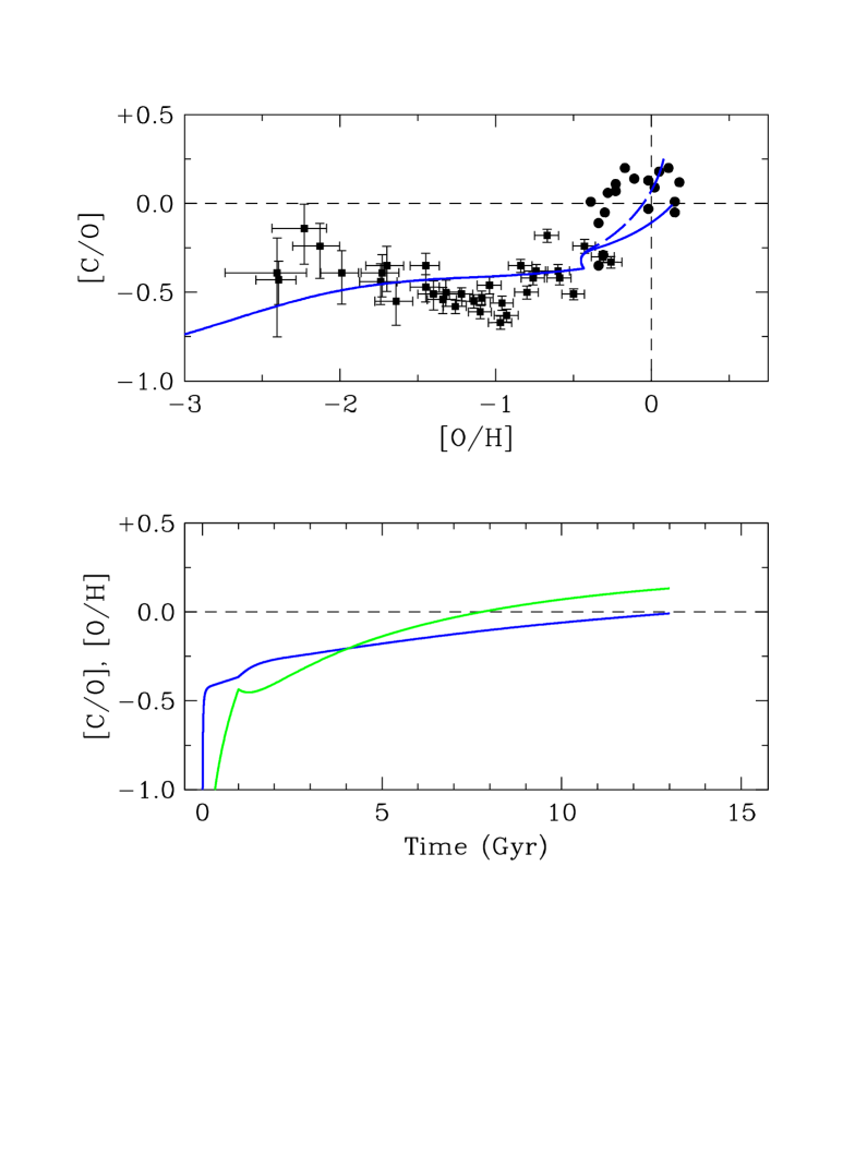
Figure 6: The outputs of our chemical evolution models are compared with the observed abundances of carbon and oxygen (dots). In the upper panel, the continuous line shows the behaviour of [C/O] vs. [O/H] produced by our ‘standard’ model, while the long-dash line shows the effect of replacing the massive star yields of Meynet & Maeder (2002) with those of Maeder (1992). In the lower panel, the black line shows the rise in [C/O] with time in the ‘standard’ model; the light grey line shows the same for [O/H].

5.4 Outputs of chemical evolution models

With the parameters described in Sections 5.1, 5.2, and 5.3 above, and interpolating the yields linearly in metallicity and stellar mass, we can follow the evolution of carbon and oxygen in the solar vicinity from 13 Gyr ago to the present. In principle, it is possible to optimise the agreement between models and observations by appropriately adjusting some of the many ingredients of the models. However, we feel that such an approach is of limited use, unless the changes involved are physically motivated. For example, it is obvious that if one were free to make ad hoc adjustments to the IMF, a better fit to the data may result. However, given the lack of empirical evidence for variations in the IMF, there is little justification for introducing this additional variable. Thus, rather than striving to obtain the best fit to the data, we are more interested in considering general trends in the behaviour of the carbon and oxygen abundances, and in what such trends can tell us about the production of these two elements.

Figure 6 shows, as a function of [O/H] and time, the [C/O] ratio computed with our ‘standard’ model which, to recap, uses the yields of Meynet & Maeder (2002) for massive stars, and those of van den Hoek & Groenewegen (1997) for low and intermediate mass stars. During the first Gyr, which in our model corresponds to the formation of the halo (Section 5.1), the oxygen abundance reaches [O/H] $\simeq-0.5$ and the [C/O] ratio grows quickly to a plateau at [C/O] $\simeq-0.5$, a value which is in approximate agreement with the ratio measured in most halo stars. At the onset of disk formation (recognisable in Figure 6 from the discontinuity in the model lines), [C/O] grows over a period of 12 Gyr by a factor of $\sim 3$ to reach solar proportions today. The agreement between the model and the measurements in disk stars can be improved if we adopt the earlier work by Maeder (1992; long-dash line in Figure 6), which used higher mass loss rates for massive stars (by factors of 2–3; see Meynet & Maeder 2000) and thus resulted in higher carbon yields than the later calculations by Meynet & Maeder (2002). This gives an indication of the uncertainties associated with theoretical yields (rather than implying that stellar rotation should not be taken into account).

Figure 7: The relative contributions to carbon enrichment from stars of different masses in our models. Left-hand panels: massive stars ($8\leq m\leq 80$ $M_{\odot}$); middle panels: low and intermediate mass stars ($0.8\leq m\leq 8$ $M_{\odot}$); right-hand panels: Type Ia supernovae (4% of stars with masses in the range $3\leq m\leq 16$ $M_{\odot}$).

The rise in [C/O] over the lifetime of the disk is due to two effects, both working in the same direction. One is the metallicity dependence of the carbon yield from massive stars. At higher metallicity, massive stars undergo greater mass loss rates with the net result that more carbon is ejected into the interstellar medium during the pre-supernova stage, before being converted into oxygen. The second is the delayed contribution to the carbon yield by low and intermediate mass stars, which take longer to evolve than massive stars. In our models, the former is always more important than the latter, as can be appreciated from inspection of Figure 7.

The question of whether massive stars, or stars of intermediate and low mass, are the major sources of carbon is still the subject of some debate. Our conclusion that the former dominate is in line with those reached in similar studies by Henry et al. (2000), Prantzos (2003b), and Carigi (2003). It contrasts, however, with the work of Chiappini et al. (2003a,b) who can reproduce the rise of [C/O] in the disk entirely with intermediate mass stars by appropriately varying the mass-loss parameter $\eta_{\rm AGB}$ in the yields by van den Hoek & Groenewegen (1997). Dray & Tout (2003) have recently published theoretical models of Wolf-Rayet stars over a range of metallicities and found comparable carbon enrichment from single WR stars and from asymptotic giant branch (AGB) stars. They concluded that whether the former or the latter are the dominant source of carbon depends strongly on the set of AGB yields adopted and on the assumed IMF.

A dominant contribution from massive stars, as illustrated in Figure 7, seems to us to be more consistent with the near-universal metallicity dependence of the [C/O] ratio, as we now explain. Essentially the same rise by a factor of $\sim 3$ exhibited by Milky Way stars when the metallicity grows from $\sim 1/10$ solar to solar is also seen in H ii regions of nearby spiral and irregular galaxies (see Figure 16 of Garnett 2003). Even in the Ly$\alpha$ forest at high redshift ($z\simeq 2-3$) there is evidence for a substantial deficiency of carbon relative to oxygen (Telfer et al. 2002). In general, other spiral galaxies, irregular galaxies, and the sources responsible for seeding the Ly$\alpha$ forest with metals will have experienced different star formation histories from that of the Milky Way. Thus, the fact that the [C/O] ratio shows approximately the same metallicity dependence in all of these different environments favours a general explanation—such as the metallicity dependence of the carbon yields via massive star winds—rather than an explanation based on time delay arguments whose effects on the trend of [C/O] with [O/H] are contingent on the details of the previous history of star formation.

5.5 Population III stars

As explained above, the rise in the [C/O] ratio with metallicity from the halo to the disk has been known for several years and has been successfully modelled by a number of previous studies (e.g. Henry et al. 2000; Carigi 2003; Chiappini et al. 2003a,b; Prantzos 2003b). None of these models, however, produces high values of [C/O] at the lowest metallicities; in all of them the general behaviour is similar to that of our ‘standard model’ in Figure 6, with [C/O] initially at very low levels and then quickly increasing to a plateau at [C/O] $\simeq-0.5$. As explained in Section 4, the new measurements presented in this paper may indicate a different scenario, with [C/O] starting at near-solar values at the lowest metallicities, and decreasing to [C/O] $\simeq-0.5$ as [O/H] grows to 1/10 of solar. At the moment, the data provide no more than a hint that this may be the case; the trend we see at low metallicities may be an artifact of small-number statistics, or a reflection of metallicity-dependent non-LTE corrections which we have not taken into account in our derivation of the C/O ratios. Nevertheless, it is instructive to consider possible explanations of this trend, should its reality be confirmed by future observations of metal-poor halo stars and theoretical calculations of the C i line formation.

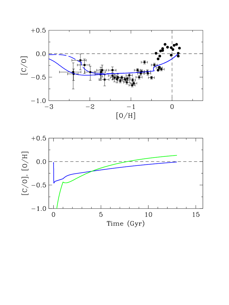
Figure 8: The outputs of our chemical evolution models obtained by adding to our ‘standard’ model yields (applicable to stars with metallicities $Z\geq 10^{-5}$) the yields by Chieffi & Limongi (2002) for metal-free stars. Continuous lines: Population III yields by Chieffi & Limongi (2002) and normal (KTG) IMF. Long-dash line: same as the continuous line, but for a top-heavy IMF ($M\geq 10M_{\odot}$). In the lower panel, the black line shows the rise in [C/O] with time for the KTG IMF case; the light grey line shows the same for [O/H].

Referring to Figure 6, it is evident that the sources of the relatively high carbon abundance must be associated with the first episodes of star formation in the Milky Way, perhaps within the first few hundred million years, when the metallicity was still very low (recall that [O/H] $=-0.5$ is reached at the end of the halo formation, after just 1 Gyr). None of the published yields for stars with metallicities $Z>0$ can reproduce [C/O] $>-0.4$ when [O/H] $<-2$, even allowing for (plausible) changes in the IMF. We are thus drawn to consider zero metallicity stars. Commonly referred to as Population III, such stars have attracted considerable attention in recent years, mostly for their cosmological importance as the first objects to form in the universe and as the sources of reionisation at $z>6$. However, their masses and chemical yields are still a matter of considerable speculation (e.g. Woosley & Weaver 1995; Heger & Woosley 2002; Chieffi & Limongi 2002; Limongi & Chieffi 2002; Umeda & Nomoto 2002).

In Figure 8 we show the results of adding to our ‘standard’ model the C and O yields by Chieffi & Limongi (2002) for metallicities in the range $0\leq Z\leq 10^{-5}$. Among the published Population III yields these are the only ones which produce the desired effect; in the combined model shown in Figure 8 the first generation of stars enriches the gas with carbon and oxygen in solar proportions and the [C/O] ratio subsequently falls as nucleosynthesis by Population II stars takes over. The nominal agreement with the observations (given the uncertainties in the current limited dataset) is improved if we assume that the IMF of Population III stars was top-heavy; as an example we show (long-dash line in Figure 8) a model with the IMF truncated at $M_{\rm low}=10M_{\odot}$ (e.g. Hernandez & Ferrara 2001; Mackey, Bromm, & Hernquist 2003; Clarke & Bromm 2003).

Chieffi & Limongi (2002) have argued on different grounds for a high carbon abundance at the end of He core burning in metal-free stars and, by inference, favour the low rate for the ¹²C ($\alpha,\gamma$) ¹⁶O reaction used in their set of nucleosynthesis calculations. Possibly, the higher temperatures reached in the cores of metal-free stars shift the balance between the ⁴He ($2\alpha,\gamma$) ¹²C and ¹²C ($\alpha,\gamma$) ¹⁶O reactions in favour of a higher carbon yield. Or perhaps the processes responsible are related to the mixing and fallback models proposed by Umeda & Nomoto (2002, 2003) to explain the abundance pattern of extremely metal-poor stars with high energy supernova explosions of massive Population III stars. In any case it is clear that, if further observations were to confirm that [C/O] really was at near-solar values in the earliest stages of the chemical evolution of the Milky Way, it would be of great interest to investigate further the physical reasons behind this effect as they would provide a much needed window into the nucleosynthesis by the first generation of stars.

6 Summary and Conclusions

We have used UVES on the VLT to measure the abundances of carbon and oxygen in 34 F and G dwarf and subgiant stars with halo kinematics and with metallicities in the range from [Fe/H] $=-0.7$ to $-3.2$ . In our study we have targeted permitted, high excitation absorption lines of C i near 9100 Å and of O i near 7774 Å which are still detectable (with equivalent widths of a few mÅ) down to the lowest metallicities in our sample. Line equivalent widths have been analysed with 1D LTE model atmospheres generated by the MARCS code to deduce values of the C/O ratio. We show that this ratio is probably insensitive to 3D effects because the lines are formed at similar deep levels within the stellar atmospheres. However, we question the suggestion by Tomkin et al. (1992) that corrections for departures from LTE are similar for the two sets of lines and the C/O ratio is therefore relatively insensitive to non-LTE effects. With more realistic estimates of the cross-sections for inelastic hydrogen collisions, differential non-LTE effects may be important (at the $\sim 0.2$ dex level) and metallicity dependent. Firm conclusions on this important point await a full study of the structure of the C i atom.

We consider our results together with those of similar studies in disk stars to investigate how the [C/O] ratio varies as a function of [O/H]. Carbon becomes proportionally less abundant than oxygen as the oxygen abundance decreases from solar; at [O/H] $\simeq-1$, [C/O] $\simeq-0.5$. This metallicity dependence of the C/O ratio is not confined to Galactic stars; a similar drop in [C/O] with [O/H] has been revealed by emission line studies of H ii regions in spiral and irregular galaxies, and by analyses of C and O absorption lines in the Ly$\alpha$ forest at high redshift. It thus appears to be a universal effect which probably reflects the metallicity dependence of the yields of carbon by massive stars with mass loss. In the Milky Way, delayed release of C by intermediate and low mass stars also contributes. We can reproduce the behaviour of [C/O] vs. [O/H] with a ‘standard’ Galactic chemical evolution model, and find that the relative contribution to carbon enrichment from stars with masses $m>8M_{\odot}$ is $\lower 2.15277pt\hbox{$\;\buildrel>\over{\sim}\;$}60$% throughout the lifetime of the Galaxy.

Our survey also provides tentative evidence for an intriguing new trend which had not been recognised before: [C/O] may rise again in halo stars with [O/H] $\lower 2.15277pt\hbox{$\;\buildrel<\over{\sim}\;$}-1$. If real, such an effect may indicate that the C/O ratio started at near-solar levels in the earliest stages of the chemical evolution of the Milky Way. Among published work on the nucleosynthesis by metal-free stars, the calculations by Chieffi & Limongi (2002) can reproduce the observed behaviour, particularly if the IMF of Population III stars was top-heavy. With the current limited statistics this is no more than a $\sim 3\sigma$ effect; it also remains to be established to what extent it is affected by systematic errors in the C/O ratios. Thus, it is now a matter of priority to confirm, or refute, the reality of such a trend, both with further observations of metal-poor halo stars and sophisticated assessment of non-LTE effects. Such tasks are well within current observational and computational capabilities; we thus look forward to a time in the relatively near future when the evolution of the C/O ratio in the Galaxy will finally be clarified.

- (1) Allende Prieto C., Lambert D. L., & Asplund M. 2001, ApJ, 556, L36
- (2) Allende Prieto, C., Lambert, D. L., & Asplund, M. 2002, ApJ, 573, L137
- (3) Alonso, A., Arribas, S., & Martínez-Roger, C. 1995, A&A, 297, 197
- (4) Alonso, A., Arribas, S., & Martínez-Roger, C. 1996, A&A, 313, 873
- (5) Andersson, H., & Edvardsson, B. 1994, A&A, 290, 590
- (6) Asplund, M., & García Pérez, A.E. 2001, A&A, 372, 601
- (7) Asplund, M., Grevesse, N., Sauval, A. J., & Allende Prieto, C. 2003a, A&A, in preparation
- (8) Asplund, M., Grevesse, N., Sauval, A. J., Allende Prieto, C., & Kiselman, D. 2003b, A&A, submitted
- (9) Asplund, M., Gustafsson, B., Kiselman, D., & Eriksson, K. 1997, A&A, 318, 521
- (10) Asplund, M., Nordlund, Å., Trampedach, R., Allende Prieto, C., & Stein, R.F. 2000, A&A, 359, 729
- (11) Asplund, M., Nordlund, Å., Trampedach, R., & Stein, R.F. 1999, A&A, 346, L17
- (12) Barklem, P.S., Belyaev, A., & Asplund, M. 2003, A&A, in press
- (13) Belyaev, A., Grosser, J.J.H., & Menzel, T. 1999, Phys. Rev. A, 60, 2151
- (14) Carigi, L. 2000, Revista Mexicana de Astronomía y Astrofísica, 36, 171
- (15) Carigi, L. 2003, MNRAS, 339, 825
- (16) Chiappini, C., Matteucci, F., & Meynet, G. 2003a, A&A, in press (astro-ph/0308067)
- (17) Chiappini, C., Matteucci, F., & Romano, D. 2001, ApJ, 554, 1044
- (18) Chiappini, C., Romano, D., & Matteucci, F. 2003b, MNRAS, 339, 63
- (19) Chieffi, A., & Limongi, M. 2002, ApJ, 577, 281
- (20) Clarke, C. J., & Bromm, V. 2003, MNRAS, in press (astro-ph/0305178)
- (21) Dekker, H., D’Odorico, S., Kaufer, A., Delabre, B., & Kotzlowski, H. 2000, in SPIE Proc. 4008, 534
- (22) Drawin, H.W. 1968, Z. Phys., 211, 404
- (23) Dray, L. M. & Tout, C. A. 2003, MNRAS, 341, 299
- (24) Eggen, O. J., Lynden-Bell, D., & Sandage, A. R. 1962, ApJ, 136, 748
- (25) ESA 1997, The Hipparcos and Tycho Catalogues, ESA SP-1200
- (26) Esteban C., Peimbert M., Torres-Peimbert S., & Escalante V. 1998, MNRAS, 295, 401
- (27) Esteban, C., Peimbert, M., Torres-Peimbert, S., & Rodríguez, M. 2002, ApJ, 581, 241
- (28) Fenner, Y., & Gibson, B. K. 2003, Publications of the Astronomical Society of Australia, in press (astro-ph/0304320)
- (29) Fleck, I., Grosser, J., Schnecke, A., Steen, W., & Voigt H. 1991, J. Phys. B, 24, 4017
- (30) Freeman, K. & Bland-Hawthorn, J. 2002, ARAA, 40, 487
- (31) Garnett, D. R. 2003, in Cosmochemistry: The Melting Pot of Elements, (Cambridge: Cambridge University Press), in press (astro-ph/0211148)
- (32) Goswami, A., & Prantzos, N. 2000, A&A, 359, 191
- (33) Gustafsson, B., Karlsson, T., Olsson, E., Edvardsson, B., & Ryde, N. 1999, A&A, 342, 426
- (34) Heger, A., & Woosley, S. E. 2002, ApJ, 567, 532
- (35) Henry, R. B. C., Edmunds, M. G., & Köppen, J. 2000, ApJ, 541, 660
- (36) Hernandez, X., & Ferrara, A. 2001, MNRAS, 324, 484
- (37) Kiselman, D. 1991, A&A, 245, L9
- (38) Kiselman, D. 1993, A&A, 275, 269
- (39) Kiselman, D. 2001, New Astron. Rev., 45, 559
- (40) Kroupa, P., Tout, C. A., & Gilmore, G. 1993, MNRAS, 262, 545 (KTG)
- (41) Limongi, M. & Chieffi, A. 2002, Publications of the Astronomical Society of Australia, 19, 246
- (42) Mackey, J., Bromm, V., & Hernquist, L. 2003, ApJ, 586, 1
- (43) Maeder, A. 1992, A&A, 264, 105
- (44) Matteucci F. 2003, Carnegie Observatories Astrophysics Series, Vol 4: Origin and Evolution of the Elements, ed. A. McWilliam & M. Rauch (Pasadena: Carnegie Observatories), in press (astro-ph/0306034)
- (45) Meynet, G. & Maeder, A. 2000, A&A, 361, 101
- (46) Meynet G., & Maeder A. 2002, A&A, 390, 561
- (47) Nissen, P. E., Chen, Y. Q., Asplund, M., & Pettini, M. 2003, A&A, submitted
- (48) Nissen, P. E., & Edvardsson, B. 1992, A&A, 261, 255
- (49) Nissen, P. E., Primas, F., Asplund, M., & Lambert, D. L. 2002, A&A, 390, 235
- (50) Oliveira, C. M., Hébrard, G., Howk, J. C., Kruk, J. W., Chayer, P., & Moos, H. W. 2003, ApJ, 587, 235
- (51) Prantzos, N. 2003a, A&A, 404, 211
- (52) Prantzos, N. 2003b, CNO in the Universe, ASP Conf. Series, eds. C. Charbonnel, D. Schaerer, & G. Meynet, in press (astro-ph/0301043)
- (53) Ryan S.G., Norris J.E., Beers T.C. 1999, ApJ, 523, 654
- (54) Salpeter, E. E. 1955, ApJ, 121, 161
- (55) Schuster, W.J., Moitinho, A., Parrao, L., & Covarrubias, E. 2003, in preparation
- (56) Schuster, W.J., & Nissen P.E. 1988, A&AS 73, 225
- (57) Sedlmayr, E. 1974, A&A, 31, 23
- (58) Stein, R.F., & Nordlund, Å. 1998, ApJ, 499, 914
- (59) Stürenburg, S., & Holweger, H. 1990, A&A, 237, 125
- (60) Telfer, R. C., Kriss, G. A., Zheng, W., Davidsen, A. F., & Tytler, D. 2002, ApJ, 579, 500
- (61) Thielemann F. K., Nomoto K., & Hashimoto M. 1993, in Origin and Evolution of the Elements, eds. N. Prantzos et al., (Cambridge: Cambridge University Press), 297
- (62) Tomkin, J., Lemke, M., Lambert, D. L., & Sneden, C. 1992, AJ, 104, 1568
- (63) Umeda, H. & Nomoto, K. 2002, ApJ, 565, 385
- (64) Umeda, H. & Nomoto, K. 2003, ApJ, submitted (astro-ph/0308029)
- (65) VandenBerg, D.A., Swenson, F.J., Rogers, F.J., Iglesias, C.A., & Alexander, D.R. 2000, ApJ, 532, 430
- (66) van den Hoek L. B., & Groenewegen M. A. T. 1997, A&AS, 123, 305
- (67) Wiese, W.L., Fuhr, J.R., & Deters, T.M. 1996, J. Phys. Chem. Ref.Data, Monograph No. 7
- (68) Woosley S. E., & Weaver T. A. 1995, ApJS, 101, 181