Relationship between environment and the broad-band optical properties of galaxies in the SDSS

Abstract

We examine the relationship between environment and the luminosities, surface brightnesses, colors, and profile shapes of luminous galaxies in the Sloan Digital Sky Survey (SDSS). For the SDSS sample, galaxy color is the galaxy property most predictive of the local environment. Galaxy color and luminosity jointly comprise the most predictive pair of properties. At fixed luminosity and color, density is not closely related to surface brightness or to Sérsic index — the parameter in this study that astronomers most often associate with morphology. In the text, we discuss what measureable residual relationships exist, generally finding that at red colors and fixed luminosity, the mean density decreases at the highest surface brightnesses and Sérsic indices. In general, these results suggest that the morphological properties of galaxies are less closely related to galaxy environment than are their masses and star-formation histories.

1 Motivation

While galaxy formation theory has had remarkable success in predicting certain properties of galaxies (their clustering, for example), it does not yet successfully predict the detailed joint distribution of galaxy properties, such as their luminosities, colors, surface brightnesses, and profile shapes. Thus, we do not have a complete understanding of the physical processes associated with galaxy formation, such as gas infall, disk dynamics, galaxy mergers, star formation, and feedback from supernovae and central black holes. However, from observations we do know that galaxy properties correlate with galaxy environment and therefore that one physical parameter of importance is the local density. A more detailed understanding of the relationship of galaxy properties to that physical parameter may therefore shed light on galaxy formation.

Much work on this subject focuses on the relationship between galaxy morphology and environment (e.g. Hubble 1936; Oemler 1974; Dressler 1980, or the more recent work of Hermit et al. 1996; Guzzo et al. 1997; Giuricin et al. 2001). These works all find that earlier type (elliptical) galaxies are more strongly clustered than later type (spiral) galaxies. Another approach is to consider clustering as a function of more objective (though not necessarily more relevant) quantities such as spectral type (Norberg et al. 2002) or photometric color, surface brightness, luminosity, or profile shape (e.g. Hashimoto & Oemler 1999; Zehavi et al. 2002). Since all the properties mentioned above (morphology, spectroscopic properties, and photometric properties) are highly correlated, it is not surprising that clustering is a function of all of them. The question naturally arises as to which properties are correlated with environment independently of the others. Norberg et al. (2002), Zehavi et al. (2002), Budavari et al. (2003), and Hogg et al. (2003) have begun this process by measuring the clustering of galaxies as a function of luminosity and other properties jointly.

In this paper we systematically explore the local environments of luminous galaxies as a function of their colors, luminosities, surface brightnesses and radial profile shapes, using the Sloan Digital Sky Survey (SDSS; York et al. 2000). Where necessary, we have assumed cosmological parameters $\Omega_{0}=0.3$, $\Omega_{\Lambda}=0.7$, and $H_{0}=100h$ km s^-1 Mpc^-1.

2 Data

The SDSS is taking $ugriz$ CCD imaging of $10^{4}~{}\mathrm{deg^{2}}$ of the Northern Galactic sky, and, from that imaging, selecting $10^{6}$ targets for spectroscopy, most of them galaxies with $r<17.77~{}\mathrm{mag}$ (e.g., Gunn et al., 1998; York et al., 2000; Abazajian et al., 2003). Automated software performs all of the data processing: astrometry (Pier et al., 2003); source identification, deblending and photometry (Lupton et al., 2001); photometricity determination (Hogg et al., 2001); calibration (Fukugita et al., 1996; Smith et al., 2002); spectroscopic target selection (Eisenstein et al., 2001; Strauss et al., 2002; Richards et al., 2002); spectroscopic fiber placement (Blanton et al., 2003c); and spectroscopic data reduction. An automated pipeline measures the redshifts and classifies the reduced spectra, modeling each galaxy spectrum as a linear combination of stellar populations (Schlegel et al., in preparation).

The sample is statistically complete, with small incompletenesses coming primarily from (1) galaxies missed because of mechanical spectrograph constraints (6 percent; Blanton et al., 2003c), which does lead to a slight under-representation of high-density regions, and (2) spectra in which the redshift is either incorrect or impossible to determine ($<1$ percent). In addition, there are some galaxies ($\sim 1$ percent) blotted out by bright Galactic stars, but this incompleteness should be uncorrelated with galaxy properties.

Galaxy luminosities and colors (measured by the standard SDSS petrosian technique; Petrosian, 1976; Strauss et al., 2002) are computed in fixed bandpasses, using Galactic extinction corrections (Schlegel et al., 1998) and $K$-corrections (computed with kcorrect v1_16; Blanton et al., 2003). They are $K$-corrected not to the redshift $z=0$ observed bandpasses but to bluer bandpasses ${}^{0.1}\!{g}$, ${}^{0.1}\!{r}$ and ${}^{0.1}\!{i}$ “made” by shifting the SDSS $g$, $r$, and $i$ bandpasses to shorter wavelengths by a factor of 1.1 (c.f., Blanton et al., 2003, 2003a). This means that galaxies at exactly redshift $z=0.1$ (typical of the SDSS sample used here) all have the trivial $K$-correction $K(z=0.1)=-2.5\log_{10}(1.1)$ regardless of their spectral energy distribution.

To determine the galaxy profile shape, we fit the radial galaxy profile using a simple Sérsic measurement (Sérsic 1968), accounting for seeing. The form of the Sérsic profile is:

$$I(r)=A\exp\left[-(r/r_{0})^{1/n}\right].$$ (1)

From a fit of the radial profile to this form, we derive a Sérsic index $n$ (which takes a value of 1 for exponential galaxies and 4 for de Vaucouleurs galaxies), half-light sizes $r_{50}$ in kpc, and surface-brightnesses of galaxies $\mu_{50}$. As described in the Appendix, our Sérsic measurements here are an updated version of those in Blanton et al. (2003a), for which there was a bias in the Sérsic indices of concentrated galaxies. From tests of simulated data processed with the SDSS photometric pipelines plus our Sérsic fitting procedure, we find that our Sérsic indices are underestimates at high Sérsic index (we measure about $n=3.5$ for input galaxies with $n=4$).

For the purposes of computing large-scale structure statistics, we have assembled a subsample of SDSS galaxies known as the NYU LSS sample10. This sample is a superset of the recent Data Release One (Abazajian et al. 2003). For each galaxy in sample10, we have computed a volume $V_{\mathrm{max}}$ representing the total volume of the Universe (in $h^{-3}~{}\mathrm{Mpc^{3}}$) in which the galaxy could have resided and still made it into the sample. The calculation of these volumes is described elsewhere (Blanton et al., 2003a).

We estimate the overdensity on $1\,h^{-1}~{}\mathrm{Mpc}$ scales from a deprojected angular correlation function. Around each spectroscopic target galaxy, galaxies are counted in the SDSS imaging in the magnitude range corresponding to $M^{\ast}\pm 1~{}\mathrm{mag}$ (passively-evolved and $K$-corrected as for an early-type galaxy) and within $5h^{-1}~{}\mathrm{Mpc}$ (transverse, proper; e.g., Hogg, 1999) at the spectroscopic galaxy redshift. We weight the count to recover the estimated overdensity averaged over a spherical three-dimensional Gaussian window $e^{-r^{2}/2a^{2}}$ with a radius of $a=1h^{-1}~{}\mathrm{Mpc}$ (proper). Eisenstein (2003) give the details of the weighting and the method for correcting for the survey mask. The results do not depend on an assumed model of the correlation function but do depend inversely on the normalization of the luminosity function at the redshift in question. One advantage of this method is that the density can be estimated with a volume-limited and yet reasonably dense set of galaxies, even at the furthest reaches of the spectroscopic catalog. Another advantage is that the estimator is not affected by redshift distortions. If the spatial correlation function $\xi(r)$ has the form $r^{-\gamma}$, then the mean overdensity around galaxies $\left<\delta_{1}\right>$ is $(2/\sqrt{\pi})\,\Gamma([3-\gamma]/2)\,\xi(1\,h^{-1}~{}\mathrm{Mpc})$, where $\Gamma(x)$ is the standard gamma function.

In what follows, the mean overdensities of a range of galaxy subsamples are presented. The mean has the advantage that it recovers a true three-dimensional overdensity, smoothed with a well-defined filter. While it is also interesting to study the properties of galaxies selected to be in environments of different overdensity (as in, e.g. Hogg et al. in preparation), the overdensity estimators used here have signal-to-noise too low for use in galaxy selection. This density estimator is generally only informative in the mean.

We selected the sample of galaxies used here to have apparent magnitude in the range $14.5<r<17.77~{}\mathrm{mag}$, redshift in the range $0.05<z<0.22$, fixed-frame absolute magnitude in the range $M_{{}^{0.1}i}>-24.0~{}\mathrm{mag}$, and enough surrounding sky area to reliably measure overdensities. These cuts left 114994 galaxies.

3 Dependence of overdensity on galaxy properties

3.1 What pair of galaxy properties is most closely related to overdensity?

In this section we demonstrate that the pair of galaxy properties (among the four we consider here) most predictive of local overdensity is color and luminosity.

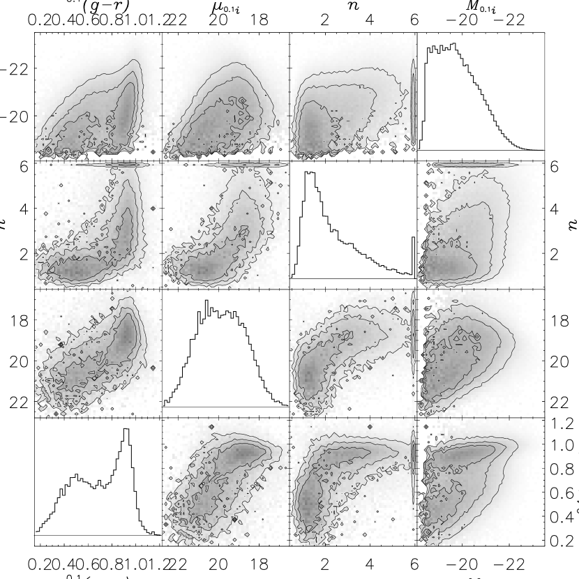
Figure 1 shows for our sample the $1/V_{\mathrm{max}}$-weighted distribution of ${}^{0.1}\!{(g-r)}$ color, half-light surface brightness $\mu_{{}^{0.1}\!{i}}$, Sérsic index $n$, and absolute magnitude $M_{{}^{0.1}\!{i}}$. The diagonal plots show the distribution of each property individually as a histogram on a linear scale; the off-diagonal plots show it as a two-dimensional histogram expressed as a grey scale. The contours on the greyscale indicate the areas containing 97%, 84% and 52% of the distribution (from the outer contours to the inner contours). This figure repeats the results of Blanton et al. (2003b) but for the more restrictive set of luminosities we consider here, and as discussed above including improved estimates of the Sérsic indices. A small number of galaxies ($<1\%$) have a best-fit Sérsic index $n=6$, corresponding to the largest value we allow.

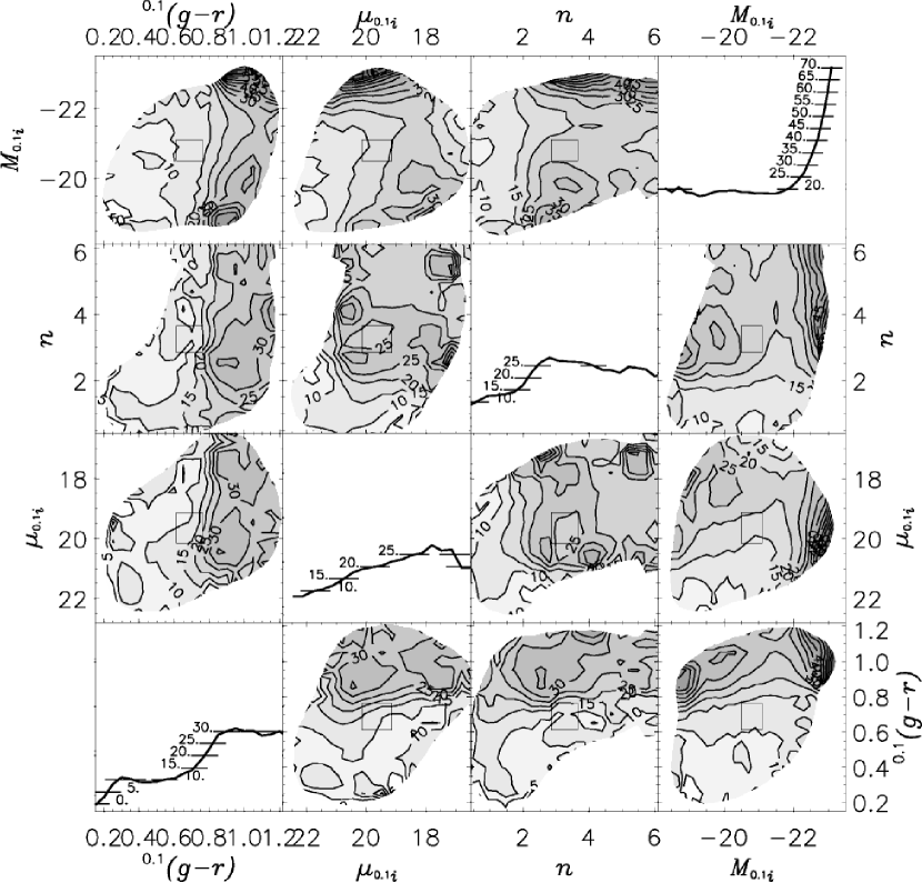
Figure 2 shows a contour plot of the mean overdensity around galaxies as a function of each property and each pair of properties. The mean is calculated in a sliding box with width $(0.15,1.0,0.8,0.6)$ in color, surface brightness, Sérsic index, and absolute magnitude respectively. The diagonal panels show the plot using a one-dimensional analog of the contour plot; the lines indicate the mean and the labeled cross bars (designed to be the width of the sliding box) indicate where the mean crosses various thresholds. In the off diagonal plots, regions colored dark indicate higher density. If the sliding box contains fewer than 200 galaxies, the result is ignored and colored pure white.

We evaluate the uncertainties in these results using the jackknife technique, dividing the survey area into ten roughly contiguous, roughly equal area sections. We then recalculate our results ten times, each time leaving out one section. The jackknife estimate of the standard deviation in the mean overdensity is the square root of the second moment of this set of results around the original result (Lupton 1993):

$${\left\langle{\Delta x^{2}}\right\rangle}^{1/2}=\left[\frac{N-1}{N}\sum_{i}(x_{i}-{\bar{x}}_{i})^{2}\right]^{1/2}$$ (2)

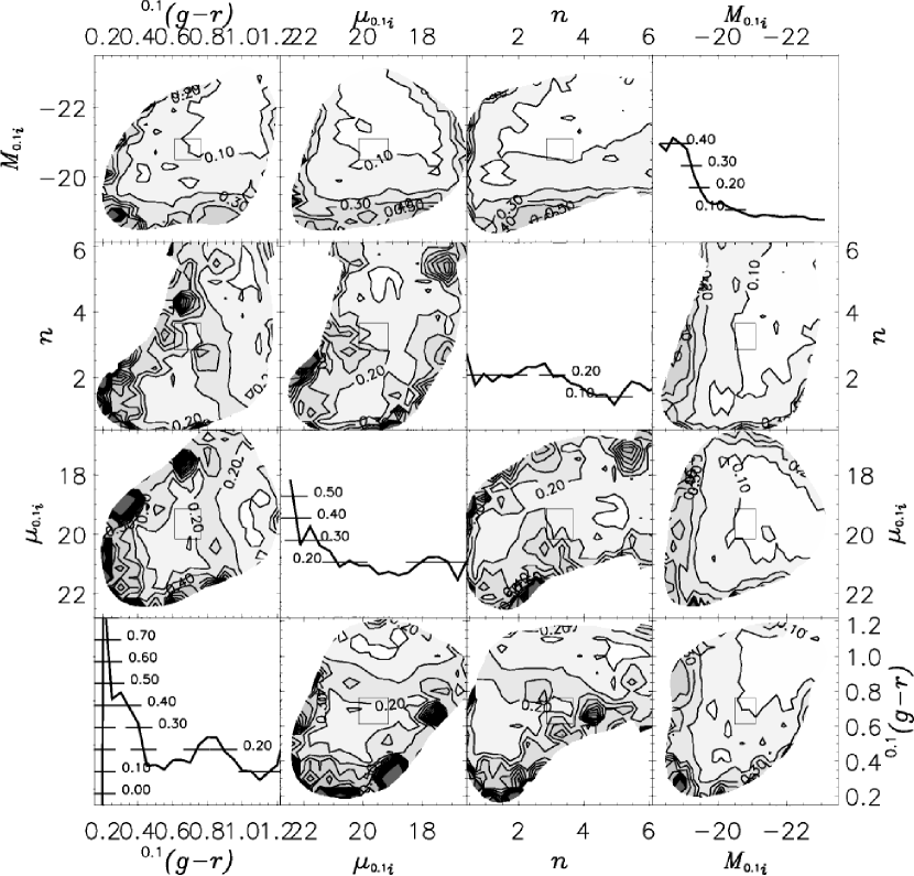
This method thus includes the effects of cosmic variance in the uncertainty budget. Figure 3 shows the standard deviation as a fraction of the mean overdensity calculated in this way. Over most of the plots the uncertainty is of order 10–30%.

What properties or pair of properties are most closely related to overdensity? This question is not completely well-defined. For example, even if the dependence of mean overdensity on galaxy properties were purely linear, the slopes of those linear relations would be impossible to compare in a meaningful way — what relates the units of Sérsic index $n$ to those of absolute magnitude $M$? One way of expressing the question that is at least independent of metric choices is to ask what property or pair of properties is most predictive of an object’s local density. That is, take the number density weighted variance of the $\delta_{1}$ measurements $\sigma^{2}\equiv{\langle{(\delta_{1,i}-{{\bar{\delta}}_{1}})^{2}}\rangle}$. Now measure ${\bar{\delta}}_{1}(X,Y,\ldots)$ as a function of one or more galaxy properties, as in Figure 2. It must be the case that

$$\sigma_{X}^{2}\equiv{\left\langle{(\delta_{1,i}-{\bar{\delta}}_{1}(X_{i}))^{2}}\right\rangle}\leq\sigma^{2}$$ (3)

As stated above, this statistic is independent of the units of the quantities $X$. It is dependent on one’s choice of binning for these quantities, but the binning we use is reasonable in the sense that each bin contains a large number of galaxies, is somewhat bigger than the errors in each parameter, and is smaller than any features in the actual distribution of the given parameter. Note that when we perform this calculation, we in fact weight each galaxy by $1/V_{\mathrm{max}}$; weighting by number density rather than luminosity density (or some other weighting) is an arbitrary choice. What parameter $X$ or pair of parameters $X$ and $Y$, minimizes this variance? Table 1 lists the values of $\sigma_{XY}-\sigma^{2}$ for each pair $X$ and $Y$.

For galaxies in the range of luminosities considered here, ${}^{0.1}\!{(g-r)}$ color is the most predictive of overdensity in this sense. In Figure 2, the dependence on luminosity appears more impressive, but this dependence only affects a small fraction of the total number density of galaxies in this sample.

The most predictive pair of properties is ${}^{0.1}\!{(g-r)}$ and $M_{{}^{0.1}\!{i}}$ taken together. The dependence of overdensity on color and luminosity takes an interesting form, as noted previously by Hogg et al. (2003). At high luminosity clustering is a strong function of luminosity. At low luminosity it is a strong function of color. Red galaxies around $M_{{}^{0.1}\!{i}\ast}\sim-21$ are less clustered in general than red galaxies of higher or lower luminosity.

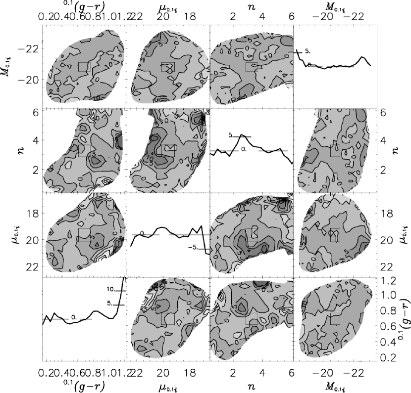
Sérsic index $n$ and surface brightness $\mu_{{}^{0.1}\!{i}}$ are both correlated with luminosity and color. Therefore, one should ask whether the remaining dependence of mean overdensity on these two parameters in Figure 2 are really independent of the dependence on luminosity and color or whether we can express the former as a consequence of the latter. To do so, we assign each galaxy in our sample a “fake” overdensity based on the mean overdensity and its variance given its luminosity and color, using the lower right panel of Figure 2. In Figure 4 we show the dependence of the mean of this fake overdensity as a function of all parameters. The form of the lower right panel is reproduced, although the dependence is slightly smeared because of the finite resolution of the grid we use to assign the fake overdensity. Figure 5 shows the difference between the actual mean overdensity in Figure 2 and the “fake” mean overdensity in Figure 4.

From Figures 4 and 5 we see that we can express some of the dependence of overdensity on Sérsic index and surface brightness in terms of the dependence on color and luminosity. For example, at low luminosity there is a dependence of overdensity on increasing Sérsic index and increasing surface brightness apparent in Figure 4, indicating that the similar dependence seen in Figure 2 is not independent of color and luminosity.

However, Figures 4 and 5 make it clear that some features of Figure 2 are independent of color and luminosity. At high luminosity, overdensity increases in Figure 2 towards lower surface brightness while overdensity remains constant in Figure 4. In Figure 5, this result appears as an increase in density towards low surface brightness at high luminosity.

We have looked at corresponding plots using all the other pairs of properties on which to base the “fake” overdensities. Unless luminosity is included explicitly as a member of the pair, the strong luminosity dependence for galaxies more luminous than $L_{\ast}$ and the lack of dependence on luminosity for less luminous galaxies cannot be replicated. Thus, this luminosity dependence is fundamental — not a derivative of the dependence on any other property. The combination of surface brightness and luminosity fails to reproduce the color and Sérsic index dependence or to reproduce the high overdensities of the red, low luminosity galaxies. The combination of Sérsic index and luminosity reproduces the dependence on surface brightness but fails to reproduce the strong dependence of density on color or (again) the high overdensities of red, low luminosity galaxies.

3.2 What is the residual dependence on the other properties?

The previous subsection shows that color and luminosity are most predictive of a galaxy’s overdensity. However, it also suggests that there is a residual dependence on Sérsic index and surface brightness. Here we explore this residual dependence in more detail.

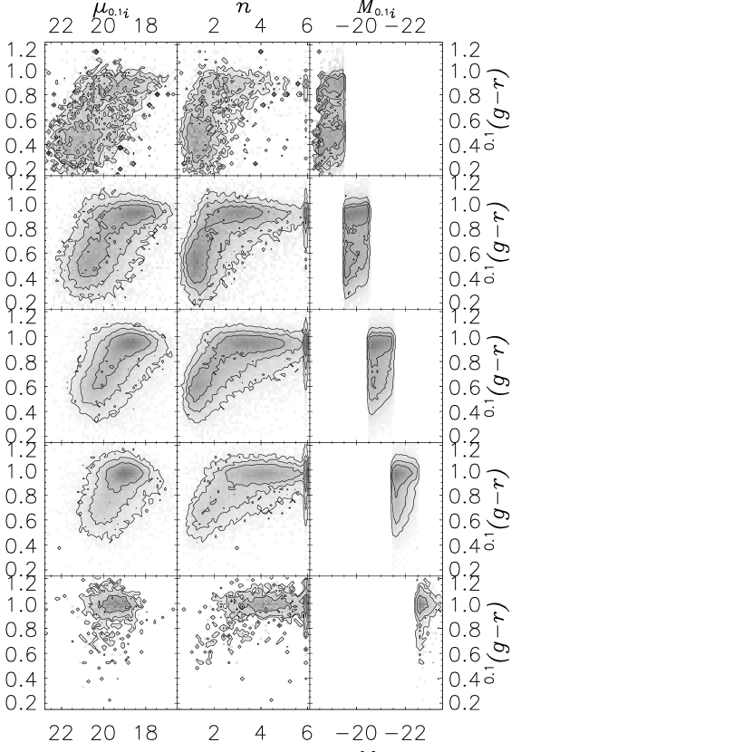
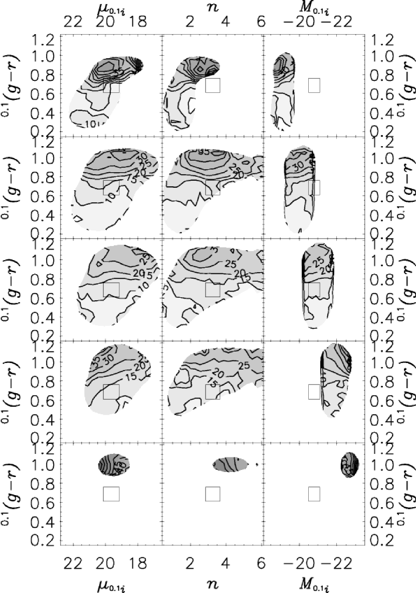
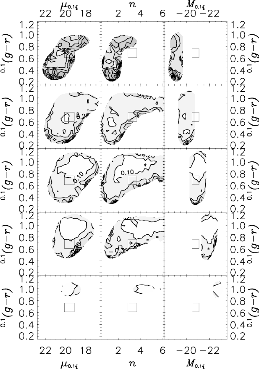
Figure 6 shows the number density distribution of galaxies as a function of color, surface brightness, and Sérsic index, for five ranges of absolute magnitude (analogously to Figure 1). Figure 7 shows the mean local overdensity for these sets of galaxies (analogously to Figure 2). The right column consists simply of slices of the lower right panel of Figure 2. However, the left two columns now show the dependence of overdensity on color and surface brightness and Sérsic index for fixed absolute magnitude. In Figure 8 we show the fractional standard deviation estimated from jackknife (analogous to Figure 3).

At high luminosity, there is dependence of overdensity on surface brightness and Sérsic index — lower surface brightness and less concentrated galaxies are in denser regions. The surface brightness dependence persists to luminosities just above $L_{\ast}$ and exists even for blue (${}^{0.1}\!{(g-r)}\sim 0.6$) galaxies.

At luminosities less than $L_{\ast}$ there is no dependence on surface brightness for blue galaxies but for red galaxies higher surface brightness galaxies exist in denser environments. Meanwhile, there is also little dependence on Sérsic index for blue galaxies of these luminosities, but for red galaxies a middle value $n=3$ of the Sérsic index indicates denser regions.

In order to test the significance of this effect, we selected galaxies with ${}^{0.1}\!{(g-r)}>0.9$, $-21.8<M_{i}<-20.2$, and $2<n<4$, regressed the overdensities of these galaxies against Sérsic index $n$, and evaluated the uncertainties in the measured slope using the jackknife samples. We found that in this range $\delta_{1}\approx 41-4.3n$, where the 1$\sigma$ uncertainties on the slope were $\sigma\sim 1.1$. Thus, this result appears significant. On the other hand, it is worth noting the caveat that this statistical measurement is a posteriori selected as interesting, out of a large number of possible measurements.

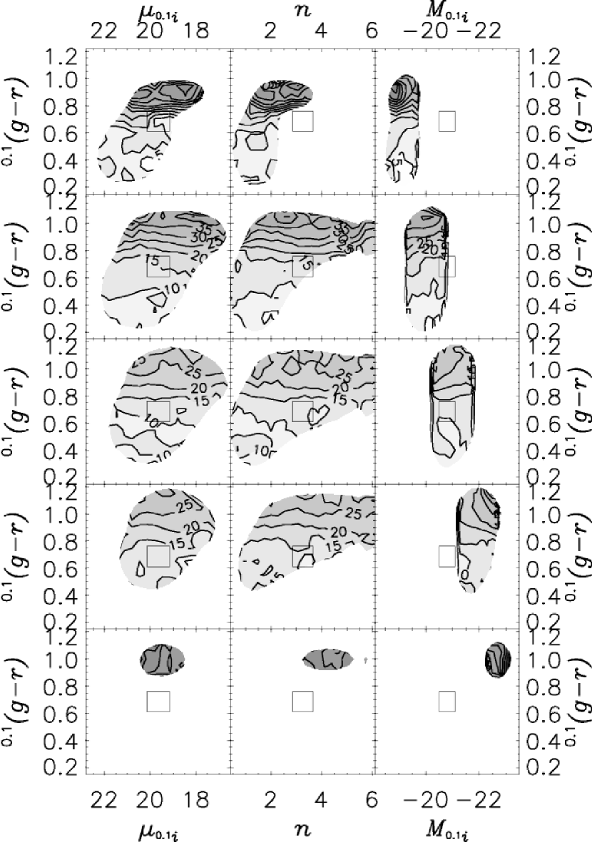
One might worry that because the slices in absolute magnitude in Figure 7 are not infinitely thin, some of the dependence on Sérsic index and surface brightness in Figure 7 is simply a result of the absolute magnitude dependence combined with the correlation of absolute magnitude with Sérsic index and surface brightness. Using the same technique as for Figure 4, we show in Figure 9 the results using the fake overdensities based on the color and absolute magnitude of each galaxy. It is clear from this figure that little of the dependence in Figure 7 results from this effect. In addition, we have repeated the test described in the last paragraph using narrower ranges of absolute magnitude and found consistent results.

4 Summary and Discussion

We have found here that the dependence of environment on color and luminosity has a nontrivial form and captures much of the interesting dependence of environment on galaxy properties. In particular, the measurement we make which is most closely related to morphology, the Sérsic index, appears to be less related to environment than is color. This result does not exclude the possibility that more detailed measurements of morphology may have a closer link with environment.

The form of our measured dependence of density on galaxy properties is likely related to phenomena already noted in the literature. The preponderance of giant ellipticals in clusters (Dressler 1980) is clearly related to the strong dependence on luminosity for red, luminous galaxies. The denseness of the environments of the lower luminosity red galaxies may be a signature of the luminous end of the dwarf elliptical population which also reside in clusters (Ferguson & Sandage 1989; de Propris et al. 1995; Mobasher et al. 2003). The strong dependence of environment on color for bluer galaxies is clearly related to the lack of star forming galaxies in clusters. In short, these results are clearly related in some way to the classical density-morphology relation. However, in our results the parameter most closely related to classical morphology (Sérsic index $n$) appears to have a relatively weak relationship with density independent of color and luminosity.

While color and luminosity are the properties most closely related to overdensity, there are some residual dependences with respect to surface brightness and Sérsic index. In particular, at high luminosity lower Sérsic index and lower surface brightness galaxies are more strongly clustered. At least part of this effect must be related to the existence of the cD galaxies at the centers of clusters, known to be less concentrated and lower surface brightness than typical giant ellipticals (Schombert 1986). However, the dependence on surface brightness persists even for blue galaxies, which cannot be caused by classical cD galaxies.

At lower luminosity, less concentrated red galaxies are more highly clustered than more concentrated red galaxies. We do not believe that this effect is related to any previously described morphology-density relationship. Nor do we believe that this result contradicts any previous investigations, none of which accounted for the interdependence of galaxy properties as systematically and completely as we have here. It is worth noting that it is possible that our photometric measurements of the Sérsic profile are being affected by nearby neighbors in such a way as to make galaxies with many neighbors appear less concentrated than the average red galaxy.

5 Future Work

The measurements we make here may be improved in two significant ways. First, we can make more detailed morphological measurements. We are currently working on more detailed morphological measurements for a nearby set of the galaxies. Second, we can push the sample to lower luminosity. Both of these efforts require considering a lower redshift sample. Unfortunately, in the current configuration of the SDSS survey it is difficult to evaluate the environments of galaxies at low redshift because of the edge effects of the survey. Nevertheless, with the Northern Galactic Cap section of the SDSS being steadily filled in, we will have a much larger contiguous data set to work on.

Here we have considered the environments of galaxies as a function of their properties, because the environmental measures we use are low signal-to-noise. However, we are working in parallel on environmental measures which are higher precision and looking at the dependence of galaxy properties as a function of their environment (Hogg et al. in preparation).

Finally, as acknowledged in Section 4, it is possible that our photometric measurements have systematic biases which are a function of environment. Although we do not believe that these effects have greatly affected our main result here that density is not strongly dependent on Sérsic index at fixed luminosity and color, we will be checking for these biases as part of a larger program of testing the photometric results of the SDSS using simulated data.

Appendix A Tests of the Sérsic Measurements

The Sérsic model fits we use here are different than those that Blanton et al. (2003b) use. We have slightly improved the Sérsic fitting code and removed a major bug. Here we describe in full the fitting method, its performance on simulated SDSS data, and the differences from the previous version.

First, we fit a model consisting of three axisymmetric gaussians to a 31x31 pixel (non-axisymmetric) image of the seeing at the center of each field determined by the SDSS Postage Stamp Pipeline (PSP; described in Stoughton et al. 2002). We equal weight the pixels in the fit and minimize the squared residuals with respect to the model parameters using the IDL routine mpfitfun, an implementation of the Levenberg-Marquardt method written by C. Markwardt. The radial profile of the fit is typically within a fraction $10^{-3}$ of the actual radial profile of the seeing image at all radii.

For each galaxy, we fit the axisymmetric Sérsic model of Equation (1) to the mean fluxes in annuli output by the SDSS photometric pipeline photo in the quantities profMean and profErr (Stoughton et al. 2002 list the radii of these annuli). photo outputs these quantities only out to the annulus which extends beyond twice the Petrosian radius, or to the first negative value of the mean flux, whichever is largest. In any case, we never consider data past the 12th annulus, whose outer radius is $68.3^{\prime\prime}$. We define:

$$\chi^{2}=\sum_{i}[(\mathtt{profMean}_{i}-\mathtt{sersicMean}_{i}(A,n,r0))/\mathtt{profErr}_{i}]^{2}$$ (A1)

where sersicMean${}_{i}(A,n,r0)$ is the mean flux in annulus $i$ for the Sérsic model convolved with the three-gaussian seeing model for the given field. We do not perform this convolution on the pixel grid, so while the seeing model includes the pixel convolution, it does not include it exactly. In practice we evaluate model annuli on a large grid of Sérsic radii, Sérsic indices, and Gaussian seeing widths, and when fitting interpolate off the grid. We again use mpfitfun for the minimization.

We have evaluated the performance of this algorithm in the following way. Taking a sampling of the parameters of our fits from the Main galaxy sample, we have generated about 1200 axisymmetric fake galaxy images, which we refer to as “fake stamps.” There are some subtleties to producing correct fake stamps, in particular with integrating the central few pixels. We first evaluate the Sérsic profile at the center of each pixel; then we sort the pixels by that intensity, and perform a full integration for the 36 pixels with the largest fluxes.

In order to simulate the performance of photo, we have distributed the fake stamps among SDSS fields. For each band, we convert the fake stamps to SDSS raw data units, convolve with the estimated seeing from PSP, and add Poisson noise using the estimates of the gain. We add the resulting image to the SDSS raw data at a random location on the frame, including the tiny effects of nonlinearity in the response and the less tiny flat-field variation as a function of column on the chip. We run photo on the resulting set of images to extract and measure objects and then run our Sérsic fitting code. This procedure thus includes the effects of seeing, noise, and sky subtraction. We have tested that our results remain the same if we insert images using an alternative estimate of the seeing based simply on stacking nearby stars (still fitting using our three-gaussian fit to the PSP seeing estimate).

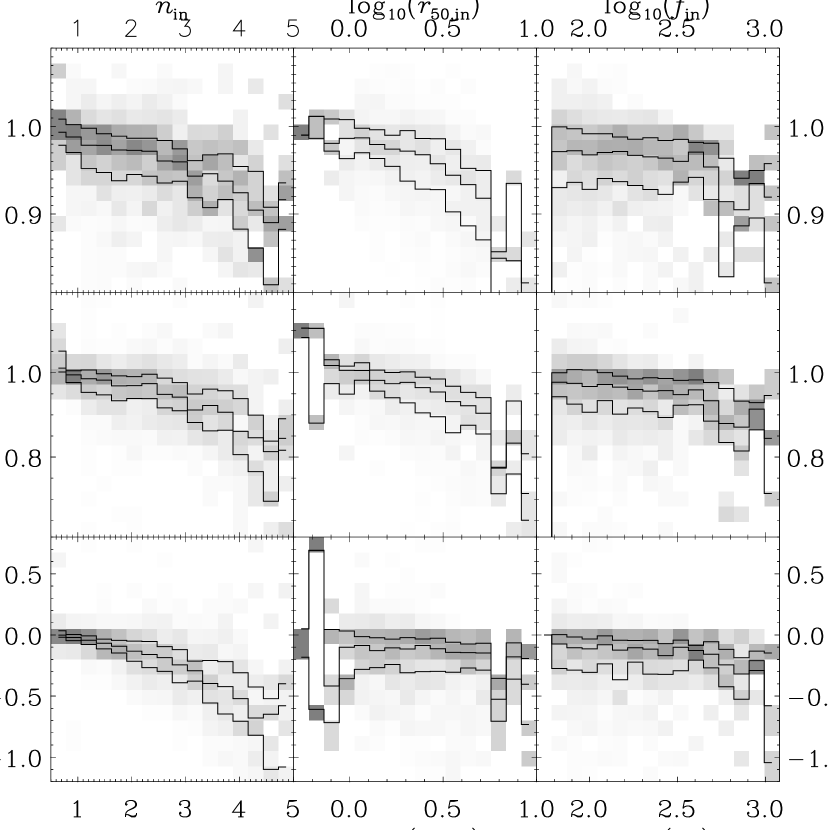
Figure 10 displays the distribution of fit parameters in the $r$-band (converting $A$ and $r_{0}$ to total flux $f$ and half-light radius of the profile $r_{50}$), as a function of the input parameters. Each panel shows the conditional distribution of the quantity on the $y$-axis as a function of quantity on the $x$-axis. The fluxes $f$ are expressed in nanomaggies, such that $f=100$ corresponds to $m=17.5$, near the flux limit of the Main galaxy sample (the general conversion of nanomaggies to magnitudes is $m=22.5-2.5\log_{10}(f)$). The lines show the quartiles of the distribution. At all Sérsic indices, sizes, and fluxes, the performance is good.

For larger sizes, sizes and fluxes are underestimated by about 10% and 15% respectively, while the Sérsic index is constant over a factor of ten in size. For high Sérsic indices, the sizes and fluxes are slightly underestimated (again by about 10% and 15%) while the Sérsic index itself is underestimated by (typically) -0.5 for a de Vaucouleurs galaxy — meaning that a true de Vaucouleurs galaxy yields $n\sim 3.5$ in our fits. This remaining bias is not much larger than the uncertainty itself and is comparable to the bias one expects (in the opposite direction) from neglecting non-axisymmetry.

The bias is partly due to our approximate treatment of the seeing, but mostly due to small errors in the sky level (at the level of 1% or less of the sky surface brightness) determined by the photometric software. If one fits for the sky level, one can recover the Sérsic indices (and fluxes and sizes) of the fake galaxies far more accurately. However, because the Sérsic model is not a good model for galaxy profiles, for real data the fits apply unrealistically high changes to the sky level to attain slight decreases in $\chi^{2}$. The resulting sizes and fluxes of the largest and brightest galaxies are obviously wrong. Thus, we satisfy ourselves that the measurements we obtain with the fixed sky level yield approximately the right answer for galaxies which are actually Sérsic models, and for other galaxies merely supply a seeing-corrected estimate of size and concentration.

When we ran this test on the original version of our code that Blanton et al. (2003b) used, we found that the Sérsic fits to de Vaucouleurs galaxies were underestimating the Sérsic index by about 1.3. This error occurred partly because we incorrectly interpreted parameters for a double Gaussian fit to the seeing produced by PSP, and somewhat less importantly, because we were not fitting explicitly for the sky level. These errors caused (relative to the fits using the new version) an underestimate in the Sérsic index for concentrated galaxies by about 0.8, and an overestimate (by up to 40%) of the galaxy size for small galaxies. Relative to the new version, the flux of the old version was underestimated by only a tiny amount ($\sim 2\%$) for concentrated galaxies and hardly at all for exponential galaxies. The old version still measured $n=1$ galaxies correctly, and for higher Sérsic indices had the property that measured Sérsic indices ran monotonically with the concentration of the galaxies.

Figure 1: Bivariate number density distributions (that is, $1/V_{\mathrm{max}}$ weighted) of properties of galaxies in our sample. All off-diagonal images have a square root stretch. Contours indicate the regions containing 52%, 84%, and 97% of the number density. The upper and lower triangles are mirror images of each other. The histograms along the diagonal show the distribution of galaxies with each property on a linear scale.

Figure 2: Mean local overdensity as a function of pairs of galaxy properties. Off-diagonals show the mean overdensity as a color-coded contour plot in which darker areas indicate galaxies in denser environments. For example, in the lower right corner, the blue, low luminosity galaxies are on average in the least dense environments and red, high luminosity galaxies are on average in the most dense environments. Plots along the diagonal show the mean overdensity as a function of each property on a linear scale. Labeled cross bars indicate where the mean crosses various thresholds.

Figure 3: Fractional uncertainties (from jackknife resampling) in the average density as a function of pairs of galaxy properties.

Figure 4: Same as Figure 2, but instead of using the actual overdensity of each galaxy, we replace it with the mean overdensity for a galaxy of that color and absolute magnitude. Thus, this figure reproduces the color and absolute magnitude dependence (slightly smeared) by design but not necessarily the other dependencies. Comparing this figure with Figure 2 reveals that the dependence on surface brightness and concentration at low luminosity is at least partly a by-product of the dependence on color at those luminosities, but that the dependence on surface brightness and concentration at high luminosity is not.

Figure 5: The difference between Figures 2 and 4, shown in the same manner as those figures.

Figure 6: Similar to Figure 1, for five ranges of absolute magnitude, as shown. Here we show only the number density as a function of color and other properties.

Figure 7: Similar to Figure 2, for the five ranges of absolute magnitude used in Figure 6. At fixed color and luminosity there exists dependencies on surface brightness and concentration. In particular, at high luminosity there is a strong dependence of clustering on surface brightness and concentration, in the sense that lower surface brightness and lower Sérsic index galaxies are in denser regions. At lower luminosity, the higher surface brightness galaxies lower Sérsic index galaxies are in denser regions.

Figure 8: Similar to Figure 3, showing fractional uncertainties in the mean overdensities plotted in Figure 7.

Figure 9: Similar to Figure 4, showing the same plot as Figure 7 but replacing the overdensity for each galaxy with the mean overdensity for its absolute magnitude and color. The correlations between density and luminosity within each luminosity slice clearly do not result in artificial features in the dependence of density on Sérsic index and surface brightness.

Figure 10: Residuals of the fit Sérsic parameters as a function of the input Sérsic parameters for a set of 1200 simulated galaxies inserted into raw data and processed with the SDSS photometric pipeline plus the Sérsic fitting procedure in Appendix A. The fluxes and sizes are those associated with the Sérsic fit. The greyscale represents the conditional probability of the $y$-axis measurement given the $x$-axis input; the lines show the quartiles of that distribution.

Table 1: Explanatory power of pairs of galaxy properties

				Property Y
Property X	$\sigma_{X}^{2}-\sigma^{2}$		${}^{0.1}\!{(g-r)}$	$\mu_{{}^{0.1}\!{i}}$	$n$	$M_{{}^{0.1}\!{i}}$
${}^{0.1}\!{(g-r)}$	-82.0		$\cdots$	-88.8	-93.3	-116.2
$\mu_{{}^{0.1}\!{i}}$	-23.8		-88.8	$\cdots$	-48.4	-46.6
$n$	-37.0		-93.3	-48.4	$\cdots$	-55.3
$M_{{}^{0.1}\!{i}}$	-4.0		-116.2	-46.6	-55.3	$\cdots$

Note. — The second column gives $\sigma_{X}^{2}-\sigma^{2}$, where $\sigma^{2}$ is the variance in the estimates of the density and $\sigma_{X}^{2}$ is the variance around the mean relations on the diagonal panels of Figure 2 for each property $X$. Each entry of the right four columns is $\sigma_{XY}^{2}-\sigma^{2}$, where $\sigma^{2}$ is the variance in the estimates of the density and $\sigma_{XY}^{2}$ is the variance around the mean relations in Figure 2 for each pair of properties $X$ and $Y$. Lower values indicate that the properties have more explanatory power; that is, that they are in this sense more related to the local overdensity. Color is the single most explanatory parameter, while color and luminosity comprise the most explanatory pair of parameters.

References

- Abazajian et al. (2003) Abazajian, K. et al. 2003, AJ, in press, (astro-ph/0305492) (Data Release One)
- Blanton et al. (2003) Blanton, M. R., Brinkmann, J., Csabai, I., Doi, M., Eisenstein, D. J., Fukugita, M., Gunn, J. E., Hogg, D. W., & Schlegel, D. J. 2003, AJ, 125, 2348
- Blanton et al. (2003a) Blanton, M. R., Hogg, D. W., Bahcall, N. A., Baldry, I. K., Brinkmann, J., Csabai, I., Eisenstein, D., Fukugita, M., Gunn, J. E., Ivezić, Ž., Lamb, D. Q., Lupton, R. H., Loveday, J., Munn, J. A., Nichol, R. C., Okamura, S., Schlegel, D. J., Shimasaku, K., Strauss, M. A., Vogeley, M. S., & Weinberg, D. H. 2003a, ApJ, 594, 186
- Blanton et al. (2003b) Blanton, M. R., Hogg, D. W., Bahcall, N. A., Brinkmann, J., Britton, M., Connolly, A. J., Csabai, I., Fukugita, M., Loveday, J., Meiksin, A., Munn, J. A., Nichol, R. C., Okamura, S., Quinn, T., Schneider, D. P., Shimasaku, K., Strauss, M. A., Tegmark, M., Vogeley, M. S., & Weinberg, D. H. 2003b, ApJ, 592, 819
- Blanton et al. (2003c) Blanton, M. R., Lin, H., Lupton, R. H., Maley, F. M., Young, N., Zehavi, I., & Loveday, J. 2003c, AJ, 125, 2276
- Budavari et al. (2003) Budavari, T. et al. 2003, ApJ, in press (astro-ph/0305063)
- de Propris et al. (1995) de Propris, R., Pritchet, C. J., Harris, W. E., & McClure, R. D. 1995, ApJ, 450, 534
- Dressler (1980) Dressler, A. 1980, ApJ, 236, 351
- Eisenstein (2003) Eisenstein, D. J. 2003, ApJ, 586, 718
- Eisenstein et al. (2001) Eisenstein, D. J. et al. 2001, AJ, 122, 2267
- Ferguson & Sandage (1989) Ferguson, H. C. & Sandage, A. 1989, ApJ, 346, L53
- Fukugita et al. (1996) Fukugita, M., Ichikawa, T., Gunn, J. E., Doi, M., Shimasaku, K., & Schneider, D. P. 1996, AJ, 111, 1748
- Giuricin et al. (2001) Giuricin, G., Samurović, S., Girardi, M., Mezzetti, M., & Marinoni, C. 2001, ApJ, 554, 857
- Gunn et al. (1998) Gunn, J. E., Carr, M. A., Rockosi, C. M., Sekiguchi, M., et al. 1998, AJ, 116, 3040
- Guzzo et al. (1997) Guzzo, L., Strauss, M. A., Fisher, K. B., Giovanelli, R., & Haynes, M. P. 1997, ApJ, 489, 37
- Hashimoto & Oemler (1999) Hashimoto, Y. & Oemler, A. J. 1999, ApJ, 510, 609
- Hermit et al. (1996) Hermit, S., Santiago, B. X., Lahav, O., Strauss, M. A., Davis, M., Dressler, A., & Huchra, J. P. 1996, MNRAS, 283, 709
- Hogg (1999) Hogg, D. W. 1999, astro-ph/9905116
- Hogg et al. (2001) Hogg, D. W., Finkbeiner, D. P., Schlegel, D. J., & Gunn, J. E. 2001, AJ, 122, 2129
- Hogg et al. (2003) Hogg, D. W. et al. 2003, ApJ, 585, L5
- Hubble (1936) Hubble, E. P. 1936, The Realm of the Nebulae (New Haven: Yale University Press)
- Lupton (1993) Lupton, R. 1993, Statistics in theory and practice (Princeton, N.J.: Princeton University Press, —c1993)
- Lupton et al. (2001) Lupton, R. H., Gunn, J. E., Ivezić, Z., Knapp, G. R., Kent, S., & Yasuda, N. 2001, in ASP Conf. Ser. 238: Astronomical Data Analysis Software and Systems X, Vol. 10, 269–??
- Mobasher et al. (2003) Mobasher, B., Colless, M., Carter, D., Poggianti, B. M., Bridges, T. J., Kranz, K., Komiyama, Y., Kashikawa, N., Yagi, M., & Okamura, S. 2003, ApJ, 587, 605
- Norberg et al. (2002) Norberg, P. et al. 2002, MNRAS, 332, 827
- Oemler (1974) Oemler, A. 1974, ApJ, 194, 1
- Petrosian (1976) Petrosian, V. 1976, ApJ, 209, L1
- Pier et al. (2003) Pier, J. R., Munn, J. A., Hindsley, R. B., Hennessy, G. S., Kent, S. M., Lupton, R. H., & Ivezić, Ž. 2003, AJ, 125, 1559
- Richards et al. (2002) Richards, G. et al. 2002, AJ, 123, 2945
- Schlegel et al. (1998) Schlegel, D. J., Finkbeiner, D. P., & Davis, M. 1998, ApJ, 500, 525
- Schombert (1986) Schombert, J. M. 1986, ApJS, 60, 603
- Sérsic (1968) Sérsic, J. L. 1968, Atlas de Galaxias Australes (Cordoba: Obs. Astronómico)
- Smith et al. (2002) Smith, J. A., Tucker, D. L., et al. 2002, AJ, 123, 2121
- Stoughton et al. (2002) Stoughton, C. et al. 2002, AJ, 123, 485
- Strauss et al. (2002) Strauss, M. A. et al. 2002, AJ, 124, 1810
- York et al. (2000) York, D. et al. 2000, AJ, 120, 1579
- Zehavi et al. (2002) Zehavi, I. et al. 2002, ApJ, 571, 172