The impact of unresolved binaries on searches for white dwarfs in open clusters

Abstract

Many open clusters have a deficit of observed white dwarfs (WDs) compared with predictions of the number of stars to have evolved into WDs. We evaluate the number of WDs produced in open clusters and the number of those WDS detectable using photometric selection techniques. This calculation includes the effects of varying the initial-mass function (IMF), the maximum progenitor masses of WDs, and the binary fraction. Differences between the calculated number of observable WDs and the actual number of WDs observed in a specific cluster then indicate the true deficit of WDs that must be explained through effects such as dynamical evolution of the cluster or close binary evolution. Observations of WDs in three open clusters, the Hyades, Pleiades, and Praesepe, are compared to the calculated observable populations in those clusters. The results suggest that a large portion of the white dwarf deficit may be explained by the presence of WDs in unresolved binary systems. However, the calculated WD populations still over-predict the number of observable WDs in each cluster. While these calculations cannot determine the cause of this residual white dwarf deficit, potential explanations include a steep high-mass IMF, dynamical evolution of the cluster, or an increased likelihood of equal-mass components in a binary system. Observations of complete WD samples in open clusters covering a range of ages and mass can help to distinguish between these possibilities.

1. Introduction

White dwarfs (WDs) are the final endpoint of stellar evolution for the vast majority of stars. WDs are gaining importance in tracing the history of stellar populations in the galaxy, including the galactic disk (e.g. Winget et al., 1987), open star clusters (e.g. Richer et al., 1998), and globular star clusters (Hansen et al., 2002). WDs are also useful in studies of supernova physics, as the upper mass of WD progenitors represents the critical progenitor mass ($M_{crit}$) for core-collapse supernovae. The value of $M_{crit}$ is relatively uncertain, with the best estimates of $5.5M_{\sun}\lesssim M_{crit}\lesssim 10M_{\sun}$.

The first significant population of white dwarfs (WDs) in open clusters was identified by Eggen & Greenstein (1965) in the Hyades (catalog ), Praesepe (catalog ), and the Pleiades (catalog ). Tinsley (1974) compared the number of Hyades WDs to the estimated number of Hyades stars having completed their lifetimes. Her work found that the WD numbers are compatible with $M_{crit}\sim 4M_{\sun}$, though this determination depends sensitively on the assumed initial-mass function (IMF), the turnoff mass of the Hyades, and the Hyades distance modulus. This value of $M_{crit}$ is lower than current lower limits ($M_{crit}\gtrsim 6M_{\sun}$), set in large part by the existence of LB 1497 (catalog ), the lone WD in the Pleiades (catalog ) (turnoff mass $\sim 5.4M_{\sun}$).

Weidemann et al. (1992) discuss the Hyades WD population and determine a deficit of 21 WDs (28 WDs predicted versus 7 observed WDs) for $M_{crit}=8M_{\sun}$ and ascribe this white dwarf deficit to dynamical evaporation of WDs from the Hyades. Similar deficits of WDs have since been observed in other open clusters, including M67 (catalog ) (Richer et al., 1998), Praesepe (catalog ) (Claver et al. 2001, hereafter CLBK ), and NGC 2099 (catalog ) (Kalirai et al., 2001c). The existence of the white dwarf deficit is still debatable, as discussed by von Hippel (1998).

Three explanations for the white dwarf deficit in open clusters readily come to mind. First, WDs may evaporate from open clusters due to dynamical evolution. Mass segregation and galactic tidal fields alone are not sufficient to remove WDs from open clusters, as a 0.6$M_{\sun}$ WD is still more massive than typical cluster stars and thus unlikely to suffer preferential evaporation. This is borne out by modern $N$-body simulations of open clusters, such as those of Portegies Zwart et al. (2001); Baumgardt & Makino (2003) and Hurley & Shara (2003), which find that WDs remain bound in open clusters. However, if a WD receives a sufficient velocity kick from asymmetric mass loss during its post-main sequence evolution, the WD may become unbound from the open cluster. This scenario was first suggested by Weidemann et al. (1992) to explain the WD deficit in the Hyades (catalog ). Recent, simple $N$-body simulations by Fellhauer et al. (2003) confirm that this mechanism can preferentially remove WDs from an open cluster, though scant observational evidence exists.

A second explanation for the white dwarf deficit, though not exclusive of the dynamical evolutionary argument, is that the WDs may be hidden in binary systems in which the intrinsically faint WDs are not detected due to the overwhelming light of brighter companion (e.g. Kalirai et al., 2001c). Searches for WDs in binaries have been undertaken in the Hyades. Two of the known Hyades WDs, EGGR 38 (catalog ) and V471 Tau (catalog ), are in binary systems. More recently, additional Hyades WDs have been discovered hidden in unresolved binaries, including HD 27483 (catalog ) (Böhm-Vitense, 1993), VA351 (catalog ) (Franz et al., 1998), and four potential WDs in Am binary star systems (Debernardi et al., 2000). Clearly some WDs lie hidden in unresolved binary systems, but the exact numbers are not known.

The third explanation for the small number of white dwarfs seen in the Hyades and other well studied young clusters could be that our expectations of WD numbers are incorrect. The deficit discussed for the Hyades would go away if $M_{crit}$ is low ($\sim 4M_{\sun}$), if the IMF for masses above the cluster turnoff mass is steeper than the present-day mass function around the turnoff mass, or a combination of these two effects. The low value of $M_{crit}$ seems unlikely, given that WDs have been observed in clusters with turnoff masses higher than 4$M_{\sun}$, including the Pleiades, NGC 2516 (catalog ) (Koester & Reimers, 1996) and NGC 2168 (catalog ) (Reimers & Koester, 1988).

We have developed a Monte Carlo method of calculating the number of WDs detectable in observations of specific open clusters, a calculation designed to aid in the interpretation of data from the Lick-Arizona White Dwarf Survey (LAWDS, Williams & Bolte, 2003) and could be used in conjunction with other ongoing cluster WD surveys, such as the CFHT Open Cluster Survey (Kalirai et al., 2001a) and the WIYN Open Cluster Study (von Hippel & Sarajedini, 1998). This calculation utilizes the observed characteristics of specific open clusters, including the cluster age, distance and reddening, and determines how many WDs would be detected given photometric WD selection criteria. The structure of this calculation, its limitations, and tests of the calculation are presented in §2. In §3 we present the results of the calculations for the Hyades, Praesepe, and the Pleiades and compare these results to the observed WD populations. In §4 we discuss the results and discuss the usefulness of these calculations in regard to current searches for WDs in open clusters.

2. Calculating the WD populations in open clusters

The number of WDs detectable by photometric observations of open clusters can be calculated by appropriate modeling of the cluster, including the effects of unresolved binary stars, choice of IMF, WD detection criteria, $M_{crit}$, metallicity and cluster age. Assuming that such an open cluster model is sufficiently realistic, any significant difference between the calculated numbers of observable WDs and the actual numbers of observed WDs represents the “true” white dwarf deficit that must be explained by other means, such as evaporation or other dynamical evolution.

Monte Carlo techniques are used to calculate the observable WD population. Stars are randomly drawn from an input IMF. For this work, four input IMFs $\xi(M)\propto M^{-(1+\Gamma)}$ were considered: a Salpeter IMF with $\Gamma=1.35$ (Salpeter, 1955), a steeper power law that accounts for unresolved binary systems with $\Gamma=2$ (Naylor et al., 2002), and a broken power law with a flat low-mass slope: $\Gamma=0.2\,(M\leq 1M_{\sun})\,;\,\Gamma=1.8\,(M>1M_{\sun})$ (Naylor et al., 2002), hereafter called the “Naylor IMF,” and the Kroupa IMF with $\Gamma=0.3\,(M<0.5M_{\sun})\,;\,\Gamma=1.3\,(M\geq 0.5M_{\sun})$ Kroupa (2001).

Stars are assigned a binary companion with a probability based on an input binary fraction; the binary mass fraction is assumed to be random, i.e. the primary and secondary stars are drawn from the same IMF (see §2.1 below). The stars are then evolved to the input cluster age using the $Z=0.008,Z=0.019$ or $Z=0.040$ solar-scaled metallicity stellar evolutionary models of Salasnich et al. (2000). These models provide evolutionary data on stars with masses up to 20$M_{\sun}$, sufficiently massive to explore all likely values of $M_{crit}$.

Two outcomes are assumed for stars having completed their evolution. Stars with $M_{*}>M_{crit}$ undergo supernovae. Stars with $M_{*}\leq M_{crit}$ form a WD. The WD mass is determined from a linear approximation of the initial-final mass relation in Weidemann (2000),

$$M_{WD}=\frac{3}{35}M_{*}+0.414M_{\sun}\,.$$ (1)

Each WD is assigned a cooling age equivalent to the progenitor lifetime subtracted from the input cluster age. The radii, effective temperature, and surface gravities of each WD are interpolated from the carbon/oxygen models of Wood (1995, hereafter W (95)).

Photometric indices for each system are determined by summation of the flux from each component. Supernova remnants are assumed to emit no flux. WD fluxes are determined from the updated model atmospheres of Finley, Koester, & Basri (1997) graciously provided by D. Koester. Stellar fluxes are taken from the isochrones of Girardi et al. (2002) for the Salasnich et al. (2000) evolutionary models. These indices are corrected for the input distance modulus and reddening, assuming the interstellar reddening law of Rieke & Lebofsky (1985) and $R_{V}=3.1$.

Once the photometric indices for each system have been calculated, these indices are compared to the input WD photometric-selection criteria. These criteria include color indices and single-band magnitude limits, with the intention that the photometric criteria used to select WD candidates in actual observations of a given cluster are used in the simulation of that cluster. If a system meets these input photometric selection criteria, the number of detected WDs is incremented by one. If it fails to meet the selection criteria, the WD is considered undetected.

The Monte Carlo calculation continues to select stellar systems until the number of stars brighter than a limiting magnitude $V_{lim}$ reaches the input value. For example, if the cumulative luminosity function of an actual open cluster has $N_{*}$ stars brighter than $V_{lim}$, then each simulated cluster will also contain $N_{*}$ stars brighter than $V_{lim}$. $10^{4}$ realization of each cluster are used to ensure high precision in the output.

2.1. Limitations of the calculations

These calculations represent a simplified version of actual open clusters. The simulation assumes that all binary stars are unresolved, an assumption whose validity depends strongly on the cluster distance and the distribution of physical separations among binary stars. Binary interactions during stellar evolution, such as mass transfer systems, common envelope stages, cataclysmic variables, and the potential disruption of binaries due to mass loss are ignored. Open cluster dynamical evolution, such as evaporation of stars and evolution of the binary fraction, is also ignored. The binary mass ratios are assumed to be random, which is likely not be the case for close binaries, but is reasonable for wider binaries (Mason et al., 1998; Abt, Gomez, & Levy, 1990). Finally, stellar systems with more than two components are not considered.

Ignoring binary-star evolution and the different mass ratios of close binaries than a random IMF results in far fewer double-degenerate systems being created than as seen in realistic $N$-body simulations, such as the significant double-degenerate population seen in Hurley & Shara (2003). The presence of any observed double-degenerate sequence in an open cluster therefore can provide a constraint on the relative importance of close-binary evolution in open clusters.

The lack of consideration of dynamical evolution is not a deficiency in the calculations, but rather is one purpose of these calculations – to determine the actual number of missing WDs that dynamical evolution must be invoked to explain. The strong, observed evaporation of low-mass stars has no great impact on this calculation. Low-mass stars in binaries with a (comparatively) high-mass WD should not be affected greatly by evaporation processes, and low-mass stars not in a binary system with a WD are not used in the calculation beyond the initial selection of cluster stars.

In short, these calculations are not a simulation of WDs in the larger sense of open cluster evolution. Rather, this calculation provides a more sophisticated means of comparing the observed WD populations of specific open clusters to the expected observable WD population. Any differences between the actual observed WD population and the calculated observable population provide a measure of the strength of the dynamical evolution of the WD population.

2.2. Trials of the calculations

We ran numerous tests to verify that these calculations return reasonable results for certain limiting cases. Fig. 1 shows the output IMF of a single simulated cluster with 5000 stars more massive than 1$M_{\sun}$ for each of the input IMFs. As one would hope, the output IMFs agree with the input IMFs.

Figure 1.— Simulated initial-mass functions. Histograms indicate the output for a Salpeter IMF (solid), a $\Gamma=2$ power-law IMF (dotted), Naylor IMF (long-dashed) and Kroupa IMF (dash-dotted). Lines indicate the expected number of stars for each IMF.

Simulated clusters with a $\Gamma=2$ power-law or the Naylor IMF are found to contain fewer WDs than those with a Salpeter or Kroupa IMF, merely due to the fact that fewer high-mass stars formed due to the steeper slope. The Naylor and Kroupa IMFs result in a higher fraction of WDs being hidden in binary systems than the single power-law IMFs due to the relatively flat low-mass IMF slope, as a companion to a WD is more likely to be higher mass and therefore more luminous than the WD.

Fig. 2 shows output color-magnitude diagrams (CMDs) for calculations of clusters at four different ages containing no binary stars. Occasional minor numerical issues arise during the interpolation of photometric indices for evolved stars due to the large changes in magnitudes with minute changes in stellar mass. These issues arise primarily at inflection points in the isochrones, such at the helium flash and at the tip of the AGB. These errors do not affect the simulated detection of WDs, as both the correct and erroneous magnitudes for these stars are bright enough to hide any WD companions, and the number of stars affected is very small.

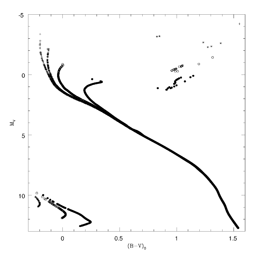
Figure 2.— $\bv,\,M_{V}$ CMD for simulated clusters of various ages. Simulated ages are for logarithmic cluster ages of 7.5 (pluses), 8.0 (asterisks), 8.5 (open circles), and 9.0 (filled squares). Simulated clusters have 1000 existing stars more massive than 1$M_{\sun}$.

The effect of the addition of binary stars is shown in Fig. 3. The sequence of binaries consisting of two main-sequence (MS) stars is readily visible in the $\bv,M_{V}$ CMD. The fan of points leading from the MS to the WD cooling sequence is composed of MS-WD binaries. The $\bv,\ub$ color-color diagram illustrates the advantage of three-band photometry over two-band photometry. The WD-MS binaries, which would blend in with background disk MS stars in a $\bv,V$ CMD, are well-separated from the locus of main-sequence in color-color space. In addition, the color-color space information clearly separates the WD cooling sequence from massive MS stars.

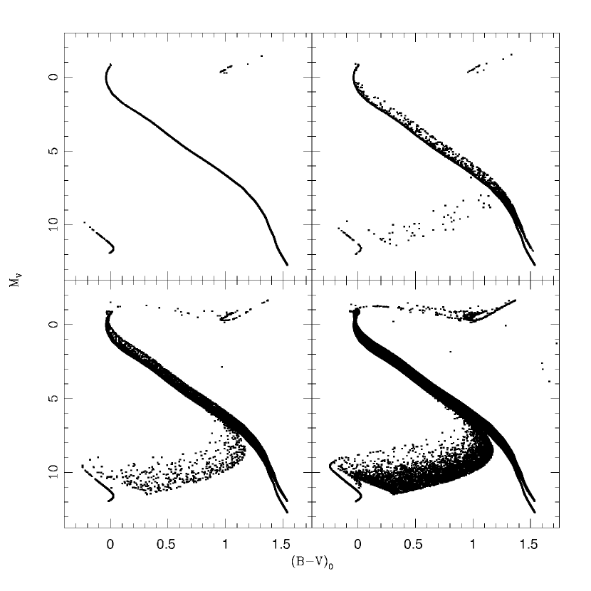
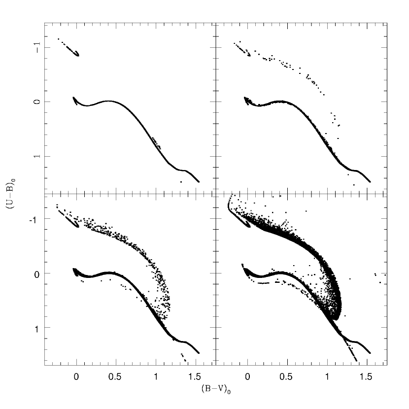
Figure 3.— $\bv,\,M_{V}$ CMD (left) and $\bv,\,\ub$ color-color diagram (right) for simulated clusters with binary stars. For each diagram, the number of stars more massive than 1$M_{\sun}$ is 1000 (top panels), $10^{4}$ (bottom left) and $10^{5}$ (bottom right). The top left panel in each diagram is for a simulated cluster with no binary stars; the binary fraction for each of the other panels is 0.5. The WD-WD binary sequence is visible in the lower right panel of the CMD, 0.75 mags brighter than the lone WD cooling sequence. Each simulation is of a cluster with a logarithmic age of 8.50 and the broken power-law IMF.

A WD-WD binary sequence is visible only when the number of stars in a cluster is very high, as seen in the lower-right panel of CMD in Fig. 3. Any significant observed WD-WD binary population in open clusters would therefore confirm that the binary component mass ratios are not random and/or that dynamical processes such as binary interactions are not negligible. Hurley & Shara (2003) find evidence of a WD-WD sequence in the photometry of NGC 6819 of Kalirai et al. (2001b).

Multiple ($10^{4}$) realizations of each cluster are used to calculate precise means and standard deviations for various categories of WDs, including the total number of WDs, the total observed number of WDs, the number of WDs in binary systems, etc.

3. Simulations of specific clusters

We have calculated the predicted observed WD populations for three open clusters: the Hyades, the Praesepe, and the Pleiades. The output populations are compared to the number of observed WDs in each system. The calculated numbers of WDs in each cluster fulfilling various criteria, including whether the WD met the photometric selection criteria (these are given individually for each cluster below), whether a WD was in a binary system, and WD progenitor masses were calculated, and the mean and standard deviation of each over the ensemble of trials were calculated.

The standard deviations are found to be nearly equal to those expected from Poisson statistics. Therefore, we use Poisson statistics to compare the calculated populations to observations of the actual cluster WDs. The probability $P$ of obtaining the actual number of observed WDs in a category or fewer is calculated from Poisson statistics given the mean value obtained from the Monte Carlo calculation. If $P\leq 0.05$, then the derived WD population is considered to be inconsistent with the observed population. For probabilities $0.15\geq P>0.05$, the calculated is termed to be mildly inconsistent with the data.

The Hyades — The Hyades (catalog ) is the open cluster with the best-studied WD system. Nine WDs are traditionally considered cluster members, though some questions as to the membership of some of these have been raised (Weidemann et al., 1992). Of these, the seven lone WDs and the WD-MS binary EGGR 38 (catalog ) are detectable as blue excess objects in $U\!BV$photometry.

For the Monte Carlo realizations the Hyades, the following physical parameters are used. The intrinsic distance modulus is assumed to be 3.33 (Perryman et al., 1998), the color excess $E(\bv)=0.01$ (Mermilliod, 1995), and the logarithmic age is assumed to be 8.80 (Perryman et al., 1998). The binary star fraction is chosen to be 0.4, approximately the lower limit of $0.41\pm 0.05$ determined from the combination of speckle, spectroscopic, and direct imaging surveys (Patience et al., 1998).

The Hyades WDs have been detected and confirmed through a variety of photometric, spectroscopic, and astrometric surveys, and a direct comparison of these selection criteria with the calculated population is not performed. In order to determine if a cluster WD is to be considered observable, we apply the photometric criteria of $\ub\leq 0.0$ and $\bv\leq 0.6$ to select WDs. These values encompass the range of indices observed in the WD sample of Eggen & Greenstein (1965), including the seven single Hyades WDs and the binary EGGR 38 (catalog ). The MS-WD binaries not selected via these criteria represent the contribution of binaries to the WD deficit.

The metallicity of the Hyades is super-solar, with $[\mathrm{Fe}/\mathrm{H}]=0.14\pm 0.05$ (Perryman et al., 1998), corresponding to $Z=0.034$ for a solar $Z=0.0245$ (Christensen-Dalsgaard et al., 1996). We therefore calculate WD populations for each of two metallicities, $Z=0.019$ and $Z=0.040$, for comparison. The calculated population also explores three values of $M_{crit}$, 10$M_{\sun}$, 8$M_{\sun}$, and 6$M_{\sun}$, bracketing the range of likely values. Finally, the calculations were performed using each of the four IMFs discussed above.

Each realization of the cluster contains 138 stellar systems in the magnitude range $3.0\leq B\leq 10.0$, consistent with the Hyades luminosity function of Oort (1979), a complete luminosity function of the Hyades upper main sequence. The resulting WD populations of the Hyades are given in Table 1.

Our results indicate that the eight photometrically-selected Hyades WDs are inconsistent ($P\leq 0.03$) with what would be expected from a Salpeter or Kroupa IMF, independent of the value of $M_{crit}$. However, the calculated number of WD detections for the $\Gamma=2$ power-law IMF and the Naylor IMF are fully consistent with the observed number of WDs for $Z=0.019$, and consistent ($P\approx 0.2$) for $Z=0.040$. The lack of any observed Hyades WDs with progenitor masses $\geq 4M_{\sun}$ (Weidemann et al., 1992; CLBK, ) is mildly inconsistent for the $\Gamma=2$ power law and Naylor IMFs at $M_{crit}=6M_{\sun}$ ($P=0.13$ and $P=0.07$, respectively) and for the $\Gamma=2$ power-law IMF for $M_{crit}=8M_{\sun}$ ($P=0.07$), but is inconsistent with the survey results for the remaining explored parameter space. This result will be explored in the discussion (§4) below.

Of the eight photometrically-detectable Hyades WDs, one is in a binary system. This is inconsistent with the number of binaries detectable from a Salpeter IMF ($P\lesssim 0.05$) and mildly inconsistent with the Kroupa IMF and $\Gamma=2$ power-law IMF for the binary fraction of 0.5, but is otherwise consistent with the calculations for the $Z=0.019$ systems. For $Z=0.04$, the single observed binary is inconsistent with one observed binary for each IMF except the Naylor IMF, which is fully consistent with the observations.

Böhm-Vitense (1995) reports on an IUE survey for WD companions to F stars in the Hyades, with only one WD-F star system (actually a triple system with two F stars and a WD) being detected. In our calculations, we have identified all stars meeting the B V selection criteria in that study. The average number of WD companions to these F stars are presented in the final column of Table 1. On average, $\lesssim 1$ F star-WD binary is present in a simulated cluster, fully consistent with the Böhm-Vitense (1995) results.

Praesepe — CLBK list ten candidate Praesepe (catalog ) WDs. Based on their analysis of six spectra, five are cluster WDs, and the other is a confirmed non-member. We obtained spectroscopy of two of the remaining candidates, WD 0834+209 (catalog ) and LB 1839 (catalog ), with the upgraded blue camera of LRIS (Oke et al., 1995) on the Keck 10-m telescope in December 2002. Both of these objects are found to be QSOs, with LB 1839 (catalog ) at $z=0.86$ and WD 0834+209 (catalog ) at $z=1.09$. Therefore, at most seven of the Praesepe candidates are WDs, and this is the number of Praesepe WDs used in the comparison to the calculated populations.

The realizations of the Praesepe calculations were normalized by the luminosity function of Jones & Stauffer (1991), who find 179 stars (completeness-corrected) with $2.5\leq M_{V}\leq 7.5$. While the Jones & Stauffer (1991) data extend to fainter magnitudes, CLBK find that the Padova isochrones do not match the Praesepe MS below this magnitude, and this mismatch would systematically bias our calculations.

The age and metallicity of the Praesepe are nearly indistinguishable from that of the Hyades (CLBK, ), so we adopt the Hyades logarithmic cluster age of 8.80 for Praesepe. As the metallicity was found to have only a small effect on the calculated observable number of WDs in the Hyades, we simulate Praesepe using only the Z=0.019 isochrones. The binary star fraction of the Praesepe is $\sim 0.4$ (Mermilliod & Mayor, 1999), so this value is used in the simulation.

For WD detection criteria, we require $\ub\leq 0.0$ and $\bv\leq 0.6$, limits encompassing the CLBK WD sample. As in the Hyades, the form of the IMF and $M_{crit}$ were varied. The calculated WD populations are given in Table 2.

As with the Hyades, the observed WD numbers are inconsistent with the calculated output for a Salpeter and Kroupa IMFs. The numbers of observable WDs calculated using the Naylor law IMF are consistent with the observed number for $M_{crit}=6M_{\sun}$ ($P=0.24$) but mildly inconsistent for higher values of $M_{crit}$ ($P=0.15$ and $P=0.11$ for $M_{crit}=8M_{\sun}$ and $M_{crit}=10M_{\sun}$, respectively). The $\Gamma=2$ power-law IMF simulation results are fully consistent with the observed numbers.

CLBK detected one WD with a progenitor mass $\geq 4M_{\sun}$. This number is inconsistent with a Salpeter and Kroupa IMF for all values of $M_{crit}$ ($P\leq 0.04$). The simulated number of WDs with massive progenitors is inconsistent with the Naylor IMF for $M_{crit}=10M_{\sun}$ ($P=0.05$), but consistent with the one observed WD for $M_{crit}=8M_{\sun}$ and $M_{crit}=6M_{\sun}$ ($P=0.17$ and $P=0.20$, respectively). The $\Gamma=2$ power law WD numbers are reasonably consistent with the observations for all values of $M_{crit}$.

None of the five confirmed Praesepe WDs are known to be in binary systems. If neither of the two remaining candidates is in a binary system, then the lack of binaries is inconsistent with the simulated results for a Salpeter or Kroupa IMF. The lack of binaries is mildly inconsistent ($P=0.08$) with the $\Gamma=2$ IMF, and consistent ($P\approx 0.19$) with the Naylor IMF. It is emphasized that this inconsistency is between the lack of observed WD binaries in Praesepe and the number of simulated WDs in binaries which would be detected given the stated photometric selection criteria; this discrepancy does not include the WDs in binary systems with photometric indices outside the selection criteria.

Pleiades — The Pleiades (catalog ) has one known member WD, LB 1497 (catalog ). For this cluster, we have normalized the IMF such that each simulated cluster contains 107 stars in the magnitude range $2.0\leq V\leq 10.0$, consistent with the luminosity function of the Pleiades from Jones (1970). We assume the Pinsonneault et al. (1998) distance modulus of 5.60 and reddening of $E(\bv)=0.04$. The metallicity of the Pleiades is near solar, with $[\mathrm{Fe}/\mathrm{H}]=-0.034\pm 0.024$ (Boesgaard & Friel, 1990), so we use the Z=0.019 isochrones. We adopt the Mermilliod et al. (1992) multiple-star frequency of 0.36 as the binary frequency. Age estimates of the Pleiades have shown scatter, with recent estimates between 100 Myr (Pinsonneault et al., 1998) and 125 Myr (Stauffer, Schultz, & Kirkpatrick, 1998). We therefore produce calculations for logarithmic cluster ages of 8.0 and 8.1.

The results are given in Table 3. For $M_{crit}=8M_{\sun}$ and $M_{crit}=10M_{\sun}$, the Salpeter and Kroupa IMFs are inconsistent with the one observed WD, regardless of the adopted cluster age. For $M_{crit}=6M_{\sun}$, the Salpeter and Kroupa IMFs are mildly inconsistent with the observed WD if the Pleiades have a logarithmic age of 8.1 ($P=0.12$), but are consistent for a logarithmic age of 8.0. The $\Gamma=2$ and Naylor IMFs produce WD populations mildly inconsistent with the Pleiades for $M_{crit}=10M_{\sun}$ and for the $M_{crit}=8M_{\sun},\log(\mathrm{age})=8.1$ simulations. Otherwise, these two IMFs result in WD populations consistent with the single observed WD.

4. Discussion

A few observations can be made from the comparisons between the calculated WD populations and the observed populations presented above. The calculations consistently over-predict the number of observed, color-selected WDs and the number of color-selected WDs in binary systems. However, the discrepancy between the expected number of WDs and the observed number is lower than in previous observational studies due to the inclusion of binaries in the simulation. Therefore, preferential evaporation of WDs from these clusters due to dynamical evolution need not be as severe as suggested by Weidemann et al. (1992) but cannot be ruled out. It should also be noted that the binary fractions used in this work represent the high end of the range of commonly-quoted cluster binary populations. A lower actual binary fraction would result in a larger WD deficit.

The number of observed WDs can be brought into agreement with the calculated numbers via at least four different methods. First, the slope of the IMF could be steeper than the slopes used here. Second, the binary fractions may be higher, resulting in more WDs being hidden in unresolved binaries. Third, the binary mass ratio could be closer to unity than the random parings discussed here, which would result in more binary WDs being hidden in systems. Fourth, some sort of dynamical evolution may be removing WDs from the open clusters. From the simulation alone, it is not possible to differentiate between these scenarios.

As mentioned above, the lack of observed WDs in the Hyades and Praesepe with progenitor masses $\gtrsim 4M_{\sun}$ is inconsistent with the calculated populations. A steeper high-mass IMF would explain the lack of these WDs, as would dynamical evolution. However, there is some evidence that binary stars in this mass range tend to have a fairly flat distribution of mass ratios, especially for orbital periods $\lesssim 0.1{\rm yr}$ (Abt, Gomez, & Levy, 1990; Mason et al., 1998). If this is true, WDs with massive progenitors may be more likely to be in binary systems with massive, unevolved stars than in binary systems with fainter, low-mass stars, and therefore more likely to go undetected.

There are several avenues of research which could shed some light on these issues. First, systematic, thorough searches for WD-mass companions to stars in the Hyades and Praesepe are needed to complete the census of WDs in each cluster, thereby determining whether or not binary systems can account for the majority of “missing” WDs in open clusters. Such a survey could include a combination of spectroscopic and high-resolution imaging (e.g. speckle and adaptive optics surveys) of these clusters, such as those published in Patience et al. (1998) and similar surveys. These surveys could also determine if the binary mass ratios for any close binaries are non-random, as opposed to the random ratios assumed in this work.

Also, WD searches in open clusters of a wide range of ages, such as the LAWDS survey we are currently undertaking, can provide evidence as to whether the deficit of massive WDs is increasing with time, as would be expected for dynamical evolution. In addition, detailed comparisons of clusters of similar ages but differing compactness and richness should also show differences in the white dwarf deficit if dynamical evolution of the WD population is significant.

The calculations presented here will be useful in interpreting data from the WD observational programs. Most importantly, the calculations permit us to estimate how strong the white dwarf deficit is in a cluster, given basic assumptions about the IMF and binary fraction. This provides a better estimate on the significance of any apparent deficit and the cluster-to-cluster variations in the deficit than could be gleaned from simpler WD population estimators, such as simple integration of the IMF.

Table 1Simulation of the Hyades.

$M_{crit}$	Z	Binary	IMF		$N_{WD}$	$N_{WD}$	$N_{WD}$	$N_{WD,F}$
($M_{\sun}$)		Fraction				in binaries	($M_{i}>4M_{\sun}$)
8	0.019	0.4	S	total	$29.7$	$16.9$	$14.2$	$0.4$
				observed	$17.5$	$4.7$	$6.7$	$\cdots$
			P	total	$14.1$	$8.0$	$5.6$	$0.07$
				observed	$9.2$	$3.2$	$2.7$	$\cdots$
			N	total	$18.9$	$10.7$	$8.0$	$0.8$
				observed	$9.8$	$1.7$	$3.6$	$\cdots$
			K	total	$31.9$	$18.0$	$15.4$	$0.8$
				observed	$16.9$	$3.3$	$7.1$	$\cdots$
		0.5	S	total	$29.9$	$19.7$	$14.2$	$0.5$
				observed	$15.5$	$5.5$	$5.4$	$\cdots$
			P	total	$14.2$	$9.5$	$5.6$	$0.08$
				observed	$8.4$	$3.7$	$2.2$	$\cdots$
			N	total	$19.2$	$12.6$	$8.1$	$0.9$
				observed	$8.4$	$2.0$	$2.9$	$\cdots$
			K	total	$32.0$	$21.1$	$15.5$	$0.9$
				observed	$14.5$	$3.8$	$5.7$	$\cdots$
	0.040	0.4	S	total	$32.2$	$18.2$	$15.1$	$0.5$
				observed	$20.7$	$7.0$	$7.6$	$\cdots$
			P	total	$15.7$	$9.0$	$6.2$	$0.077$
				observed	$11.3$	$4.6$	$3.2$	$\cdots$
			N	total	$20.6$	$11.6$	$8.6$	$0.8$
				observed	$11.3$	$2.5$	$4.0$	$\cdots$
			K	total	$34.4$	$19.3$	$16.4$	$0.9$
				observed	$19.6$	$4.9$	$7.9$	$\cdots$
6	0.019	0.4	S	total	$25.4$	$14.4$	$9.9$	$0.4$
				observed	$15.4$	$4.5$	$4.7$	$\cdots$
			P	total	$12.7$	$7.2$	$4.2$	$0.064$
				observed	$8.5$	$3.1$	$2.0$	$\cdots$
			N	total	$16.8$	$9.4$	$5.8$	$0.7$
				observed	$8.9$	$1.7$	$2.7$	$\cdots$
			K	total	$27.1$	$15.3$	$10.6$	$0.7$
				observed	$14.7$	$3.1$	$5.0$	$\cdots$
10	0.019	0.4	S	total	$32.2$	$18.2$	$16.6$	$0.5$
				observed	$18.6$	$4.8$	$7.7$	$\cdots$
			P	total	$14.9$	$8.5$	$6.3$	$0.076$
				observed	$9.6$	$3.2$	$3.0$	$\cdots$
			N	total	$20.0$	$11.3$	$9.1$	$0.87$
				observed	$10.3$	$1.7$	$4.1$	$\cdots$
			K	total	$34.5$	$19.4$	$18.1$	$0.8$
				observed	$18.1$	$3.3$	$8.3$	$\cdots$

Table 2Simulation of the Praesepe.

$M_{crit}$	IMF	$N_{WD}$	$N_{WD}$	$N_{WD}$	$N_{WD}$	$N_{WD}$	$N_{WD}$
($M_{\sun}$)		total	observed	total	observed	total	observed
				in binaries	in binaries	($M_{i}>4M_{\sun}$)	($M_{i}>4M_{\sun}$)
10	S	$35.1$	$19.7$	$19.8$	$4.8$	$18.0$	$8.4$
	P	$13.2$	$8.1$	$7.6$	$2.6$	$5.6$	$2.7$
	N	$23.0$	$11.5$	$12.9$	$1.7$	$10.4$	$4.7$
	K	$38.7$	$20.3$	$21.8$	$3.7$	$20.2$	$9.3$
8	S	$32.5$	$18.5$	$18.4$	$4.7$	$15.5$	$7.3$
	P	$12.6$	$7.9$	$7.2$	$2.6$	$5.0$	$2.4$
	N	$21.8$	$10.9$	$12.3$	$1.7$	$9.3$	$3.2$
	K	$35.7$	$18.9$	$20.1$	$3.6$	$17.3$	$8.0$
6	S	$27.8$	$16.3$	$15.8$	$4.5$	$10.7$	$5.1$
	P	$11.3$	$7.3$	$6.5$	$2.5$	$3.7$	$1.9$
	N	$19.2$	$9.8$	$10.8$	$1.6$	$6.7$	$3.0$
	K	$30.3$	$16.5$	$17.1$	$3.5$	$11.9$	$5.6$

Table 3Simulation of the Pleiades.

$M_{crit}$	log(age)	IMF	$N_{WD}$	$N_{WD}$	$N_{WD}$	$N_{WD}$
($M_{\sun}$)			total	observed	in binaries	observed in binaries
10	8.0	S	$9.1$	$7.6$	$4.8$	$3.3$
		P	$3.9$	$3.5$	$2.1$	$1.7$
		N	$5.2$	$3.6$	$2.7$	$1.1$
		K	$9.8$	$7.2$	$5.1$	$2.6$
	8.1	S	$11.3$	$9.1$	$6.0$	$3.9$
		P	$4.9$	$4.4$	$2.6$	$2.0$
		N	$6.6$	$4.4$	$3.5$	$1.3$
		K	$12.1$	$8.6$	$6.4$	$2.9$
8	8.0	S	$6.7$	$5.7$	$3.6$	$2.5$
		P	$2.9$	$2.7$	$1.6$	$1.3$
		N	$3.9$	$2.8$	$2.0$	$0.9$
		K	$7.2$	$5.3$	$3.8$	$2.0$
	8.1	S	$8.9$	$7.3$	$4.7$	$3.2$
		P	$4.1$	$3.6$	$2.2$	$1.8$
		N	$5.3$	$3.6$	$2.8$	$1.1$
		K	$9.5$	$6.9$	$5.0$	$2.4$
6	8.0	S	$2.3$	$2.0$	$1.2$	$0.9$
		P	$1.1$	$1.0$	$0.6$	$0.5$
		N	$1.4$	$1.0$	$0.7$	$0.4$
		K	$2.4$	$1.9$	$1.3$	$0.8$
	8.1	S	$4.4$	$3.7$	$2.3$	$1.7$
		P	$2.1$	$2.0$	$1.1$	$1.0$
		N	$2.8$	$2.0$	$1.5$	$0.7$
		K	$4.7$	$3.5$	$2.5$	$1.3$

References

- Abt, Gomez, & Levy (1990) Abt, H. A., Gomez, A. E., & Levy, S. G. 1990, ApJS, 74, 551
- Baumgardt & Makino (2003) Baumgardt, H., & Makino, J. 2003, MNRAS, 341, 247
- Boesgaard & Friel (1990) Boesgaard, A. M. & Friel, E. D. 1990, ApJ, 351, 467
- Böhm-Vitense (1993) Böhm-Vitense, E. 1993, AJ, 106, 1113
- Böhm-Vitense (1995) Böhm-Vitense, E. 1995, AJ, 110, 228
- Christensen-Dalsgaard et al. (1996) Christensen-Dalsgaard, J. et al. 1996, Science, 272, 1286
- (7) Claver, C. F., Liebert, J., Bergeron, P., & Koester, D. 2001, ApJ, 563, 987 (CLBK)
- Debernardi et al. (2000) Debernardi, Y., Mermilliod, J.-C., Carquillat, J.-M., & Ginestet, N. 2000, A&A, 354, 881
- Eggen & Greenstein (1965) Eggen, O. J. & Greenstein, J. L. 1965, ApJ, 141, 83
- Fellhauer et al. (2003) Fellhauer, M., Lin, D. N. C., Bolte, M., Aarseth, S. J., & Williams, K. A. 2003, ApJ, in press
- Finley, Koester, & Basri (1997) Finley, D. S., Koester, D., & Basri, G. 1997, ApJ, 488, 375
- Franz et al. (1998) Franz, O. G. et al. 1998, Bulletin of the American Astronomical Society, 30, 1402
- Girardi et al. (2002) Girardi, L., Bertelli, G., Bressan, A., Chiosi, C., Groenewegen, M. A. T., Marigo, P., Salasnich, B., & Weiss, A. 2002, A&A, 391, 195
- Hansen et al. (2002) Hansen, B. M. S. et al. 2002, ApJ, 574, L155
- Hurley & Shara (2003) Hurley, J. R. & Shara, M. M. 2003, ApJ, 589, 179
- Jones (1970) Jones, B. F. 1970, AJ, 75, 563
- Jones & Stauffer (1991) Jones, B. F. & Stauffer, J. R. 1991, AJ, 102, 1080
- Kalirai et al. (2001a) Kalirai, J. S. et al. 2001, AJ, 122, 257
- Kalirai et al. (2001b) Kalirai, J. S. et al. 2001, AJ, 122, 266
- Kalirai et al. (2001c) Kalirai, J. S., Ventura, P., Richer, H. B., Fahlman, G. G., Durrell, P. R., D’Antona, F., & Marconi, G. 2001, AJ, 122, 3239
- Koester & Reimers (1996) Koester, D. & Reimers, D. 1996, A&A, 313, 810
- Kroupa (2001) Kroupa, P. 2001, MNRAS, 322, 231
- Mason et al. (1998) Mason, B. D., Gies, D. R., Hartkopf, W. I., Bagnuolo, W. G., Brummelaar, T. T., & McAlister, H. A. 1998, AJ, 115, 821
- Mermilliod et al. (1992) Mermilliod, J.-C., Rosvick, J. M., Duquennoy, A., & Mayor, M. 1992, A&A, 265, 513
- Mermilliod (1995) Mermilliod, J. 1995, in Information and On-Line Data in Astro-nomy, ed. D. Egret & M. A. Albrecht (Dordrecht: Kluwer), 127
- Mermilliod & Mayor (1999) Mermilliod, J.-C. & Mayor, M. 1999, A&A, 352, 479
- Naylor et al. (2002) Naylor, T., Totten, E. J., Jeffries, R. D., Pozzo, M., Devey, C. R., & Thompson, S. A. 2002, MNRAS, 335, 291
- Oke et al. (1995) Oke, J.B., et. al. 1995, PASP, 107, 375
- Oort (1979) Oort, J. H. 1979, A&A, 78, 312
- Patience et al. (1998) Patience, J., Ghez, A. M., Reid, I. N., Weinberger, A. J., & Matthews, K. 1998, AJ, 115, 1972
- Perryman et al. (1998) Perryman, M. A. C. et al. 1998, A&A, 331, 81
- Pinsonneault et al. (1998) Pinsonneault, M. H., Stauffer, J., Soderblom, D. R., King, J. R., & Hanson, R. B. 1998, ApJ, 504, 170
- Pols & Marinus (1994) Pols, O. R. & Marinus, M. 1994, A&A, 288, 475
- Portegies Zwart et al. (2001) Portegies Zwart, S. F., McMillan, S. L. W., Hut, P., & Makino, J. 2001, MNRAS, 321, 199
- Reimers & Koester (1988) Reimers, D. & Koester, D. 1988, A&A, 202, 77
- Richer et al. (1998) Richer, H. B., Fahlman, G. G., Rosvick, J., & Ibata, R. 1998, ApJ, 504, L91
- Rieke & Lebofsky (1985) Rieke, G. H. & Lebofsky, M. J. 1985, ApJ, 288, 618
- Salasnich et al. (2000) Salasnich, B., Girardi, L., Weiss, A., & Chiosi, C. 2000, A&A, 361, 1023
- Salpeter (1955) Salpeter, E. E. 1955, ApJ, 121, 161
- Stauffer, Schultz, & Kirkpatrick (1998) Stauffer, J. R., Schultz, G., & Kirkpatrick, J. D. 1998, ApJ, 499, L199
- Tinsley (1974) Tinsley, B. M. 1974, PASP, 86, 554
- von Hippel (1998) von Hippel, T. 1998, AJ, 115, 1536
- von Hippel & Sarajedini (1998) von Hippel, T. & Sarajedini, A. 1998, AJ, 116, 1789
- Weidemann et al. (1992) Weidemann, V., Jordan, S., Iben, I. J., & Casertano, S. 1992, AJ, 104, 1876
- Weidemann (2000) Weidemann, V. 2000, A&A, 363, 647
- Williams (2002) Williams, K. A. 2002, Ph.D. thesis, Univ. of California Santa Cruz
- Williams & Bolte (2003) Williams, K. A., & Bolte, M. 2003, in preparation
- Winget et al. (1987) Winget, D. E., Hansen, C. J., Liebert, J., van Horn, H. M., Fontaine, G., Nather, R. E., Kepler, S. O., & Lamb, D. Q. 1987, ApJ, 315, L77
- W (95) Wood, M. A. 1995, LNP Vol. 443: White Dwarfs, 41 (W95)