Velocity Fields as a Probe of Cosmology

Analyses of peculiar velocity surveys face several challenges, including low signal–to–noise in individual velocity measurements and the presence of small–scale, nonlinear flows. I will present three new analyses that attempt to address these inherent problems. The first is geared towards the better understanding of the estimated errors in the surveys, specifically sampling errors, and the resolution of the seeming disagreements between the surveys. Another develops a new statistic that does not suffer from the usual problems and gives robust results that are galaxy–morphology and distance–estimator independent. The third introduces a formalism that allows for the accounting of most of the non–linear signal whereby the signal to noise is increased and small–scale aliasing is removed.

1 Introduction

The best developed class of theories of structure formation is based on the assumption of small amplitude Gaussian density perturbations which grew and condensed out, becoming, by gravitational instability, galaxies, clusters of galaxies, superclusters or voids. The study of the evolution of density perturbations is the basis of all theories based on gravitational instability $\!{}^{{\bf?},{\bf?}}$. Recently, this class of theories was given a dramatic boost by the detection of appropriate temperature fluctuations in the cosmic microwave background. Further, recent work on the bispectrum measurement in the IRAS redshift catalogs $\!{}^{{\bf?}}$ shows strong signature of gravitational instability.

Statistical studies of the peculiar velocity field (those velocities in excess of the pure Hubble flow) based on the predictions of the gravitational instability scenario can potentially address many fundamental cosmological questions. Although in principle the galactic peculiar (local) velocity field holds a great promise as a direct probe of the underlying mass distribution, in practice the extraction of the information is difficult and fraught with both observational and theoretical pitfalls. Velocity surveys have irregular geometries and their boundary conditions are not usually well–known. Further, they are somewhat shallow and sample the volume discretely, non–uniformly and sparsely. Theoretically, the mapping from velocity to density is complicated by non–linear effects which necessitates various approximation schemes $\!{}^{{\bf?}}$. Indeed, small–scale aliasing and incomplete cancellations $\!{}^{{\bf?},{\bf?}}$ introduce spurious noise which masquerades as large scale signal. These effects are difficult to disentangle and thus the resulting information is unreliable $\!{}^{{\bf?},{\bf?}}$. The bottom line with respect to peculiar velocity surveys is that it is very difficult to extract cosmological information since the large–scale signal has a significant small–scale noise which is virtually impossible to model accurately.

Estimating cosmological parameters may be done by studying the large scale motions of galaxies. One advantage of this method is that the large scale velocity field probes the matter distribution in the Universe directly, and not merely the light distribution as redshift surveys do. However, to measure the velocity field one needs to make accurate distance measurements, which has proven to be quite difficult $\!{}^{{\bf?}}$. The errors in distance estimates are typically some fraction of the redshift of the sample points, which in the case of distant objects can mean that the errors are larger than the peculiar velocity being measured. This is partially rectified by measuring only the lowest moment of the velocity field, namely the bulk flow. Since the bulk flow is in a sense an average of the velocities in the sample, its error is reduced over that of an individual measurement by the square root of the number of objects $\!{}^{{\bf?},{\bf?}}$. The idea here is that in calculating low–order moments the small scale modes will be averaged out, so that the values of these moments will reflect only large–scale motion. It has been shown, however, that the sparseness of peculiar velocity data can lead to small–scale modes making a significant contribution to low–order moments through incomplete cancellation  $\!{}^{{\bf?},{\bf?}}$. Another drawback of this approach is that it utilizes only a fraction of the available information.

An alternative method is to perform a likelihood analysis using all of the velocity information $\!{}^{{\bf?}}$. An obvious danger here is that retaining small–scale, nonlinear contributions to the velocities can lead to unpredictable biases which can skew the results $\!{}^{{\bf?}}$. This method also has the disadvantage of becoming unwieldy for surveys larger than about a thousand objects. While advances in computing will make this less of a problem in the future, clearly a less time–intensive method is desirable.

The non–linear aliasing and incomplete cancellations inherent in the surveys effectively defied all attempts to extract robust cosmological information from the data. The remedies proposed in the literature, POTENT $\!{}^{{\bf?}}$; denser directional surveys $\!{}^{{\bf?}}$ and others where not satisfactory. Smoothing over the problems by introducing some averaging schemes did not work consistently. Smoothing, including Weiner Filtering $\!{}^{{\bf?}}$ provide formalisms that may or may not remove small scale irregularities. The problem is that since smoothing operations provides little or no control over what we remove and what we keep, that it is impossible to state with any degree of certainty whether the smoothed field retains the large scale signal while removing the potentially significant small scale noise.

Here I would like to discuss three programs that have been developed to address different aspects of the problems discussed above. The first attempts to better understand the error estimations inherent in velocity field surveys and to develop a scheme to compare them and see if the surveys themselves are compatible with each other within their errors and with the power spectrum of density fluctuations derived by other techniques. Another searches for a statistic that is robust and does not depend on the particular distance indicator or morphology. The last tries to deal with the problems head on, that is, to look for a statistical way to rid the surveys of their non–linearities in such a way that the large–scale signal remains intact whereas the small–scale ”noise” is being removed.

One idea proposed is to develop a more realistic error estimation for existing surveys, in particular, the understanding of the sampling errors $\!{}^{{\bf?}}$ allows for consistent bulk flow estimates for most of the bulk flow measurements within the errors (see Table 1 below). Additionally, we get an idea of how much correlation we expect between the different catalogs for a given power spectrum by calculating the normalized expectation value for their dot–product which should be close to $1$ for highly correlated surveys, zero for those that are completely uncorrelated, and $-1$ if there is a high degree of anti-correlation $\!{}^{{\bf?},{\bf?},{\bf?}}$. As we see elsewhere in this volume $\!{}^{{\bf?}}$ the bulk flow measurements of various independent surveys are fairly correlated and a reasonably consistent bulk flow vector emerges from them that is $380\pm 80$km/s towards $l=290^{o}$ and $b=10^{o}$.

Recent Large Scale Bulk Flow Measurements

Survey	Method	N	vpec	Total	l	b
			km/s	error
LP $\!{}^{{\bf?}}$	BCG	119	830	370	330	39
Willick $\!{}^{{\bf?}}$	TF	15	1060	670	275	28
SC $\!{}^{{\bf?}}$	TF	63	120	295	10	310
SMAC $\!{}^{{\bf?}}$	FP	56	690	380	260	-1
EFAR $\!{}^{{\bf?}}$	FP	49	630	410	50	10
SN $\!{}^{{\bf?}}$	SNIa	65	610	330	313	9

Table 1: When we take into account both the total error, i.e. random and sampling errors, most bulk flow measurements agree with each other. For a more detailed analysis see Hudson, M., 2003, In this volume.

Another program that seeks to address the inconsistencies between various velocity surveys results develops a statistic that is not as susceptible to small–scale aliasing and incomplete cancellations. In series of recent papers we introduced a new dynamical estimator of the $\Omega_{m}$ parameter, the dimensionless density of the nonrelativistic matter in the universe. We use the so called streaming velocity, or the mean relative peculiar velocity for galaxy pairs, $v_{12}(r)$, where $r$ is the pair separation $\!{}^{{\bf?}}$. It is measured directly from peculiar velocity surveys, without the noise-generating spatial differentiation, used in reconstruction schemes, like POTENT (see Courteau et al. 2000 and references therein). In the first paper of the series $\!{}^{{\bf?}}$, we derived an equation, relating $v_{12}(r)$ to $\Omega_{m}$ and the two-point correlation function of mass density fluctuations, $\xi(r)$. Then, we showed that $v_{12}$ and $\Omega_{m}$ can be estimated from mock velocity surveys $\!{}^{{\bf?}}$, from real data: the Mark III survey $\!{}^{{\bf?}}$ and finally $\!{}^{{\bf?}}$ a comparison of various independent surveys that use different standard candles, galaxy morphologies and surveying techniques. Whenever a new statistic is introduced, it is of particular importance that it passes the test of reproducibility. Our results pass these tests: the $v_{12}(r)$ measurements are galaxy morphology– and distance indicator–independent $\!{}^{{\bf?}}$.

Using mean relative peculiar velocity measurements for pairs of galaxies, we estimate the cosmological density parameter $\Omega_{m}$ and the amplitude of density fluctuations $\sigma_{8}$. Our results suggest that our statistic is a robust and reproducible measure of the mean pairwise velocity and thereby the $\Omega_{m}$ parameter. We get $\Omega_{m}=0.30^{+0.17}_{-0.07}$ and $\sigma_{8}=1.13^{+0.22}_{-0.23}$. These estimates do not depend on prior assumptions on the adiabaticity of the initial density fluctuations, the ionization history, or the values of other cosmological parameters.

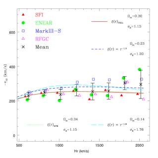
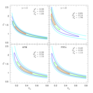
Figure 1: (left panel) The crosses and the associated error bars show the weighted mean pairwise velocity, obtained by averaging over four surveys. Individual survey data points are also shown; we have suppressed their error bars for clarity. These direct measurements of $v_{12}$ are compared to four $v_{12}(r)$ curves, derived by assuming four different models of $\xi(r)$. The labels identify best fit $\Omega_{m}$ and $\sigma_{8}$ parameters. Figure 2: (right panel) The results of the maximum likelihood analysis. The upper panels show results for power-law toy models, while the bottom panels are based on realistic representations of observations: the APM and PSCz data, respectively. Likelihood peak coordinates and the values of $\chi^{2}$ for each model are also indicated. The innermost contours define the 68%, or 1-$\sigma$ areas around the peaks. The remaining nested contours show the 2, 3 and 4-$\sigma$ boundaries.

In figure 1 $\!{}^{{\bf?}}$ we see that the claim that the $v_{12}$ statistic is independent of the galaxy morphology or the standard candle is correct. We show here four independent surveys, The Mark III $\!{}^{{\bf?}}$, a TF compilations of 2437 spiral galaxies. The SFI $\!{}^{{\bf?}}$ catalogue contains 1300 late type spiral galaxies with $I$-band TF distance estimates. The ENEAR $\!{}^{{\bf?}}$ survey with 1359 early type with $D_{n}$-$\sigma$ measured distances. The RFGC $\!{}^{{\bf?}}$ catalogue provides a list of radial velocities, HI line widths, TF distances and peculiar velocities of 1327 spiral galaxies that was compiled from observations of flat galaxies performed with the 305 m telescope at Arecibo. As can clearly be seen, all measurements agree with each other and thus allows us to combine the results and obtain a mean $v_{12}(r)$ with smaller errors than for each individual survey. Further, we see that since all surveys give us identical results within the errors, ther is no sign for velocity bias.

In figure 2 we see the results of our estimates for the parameters, $\Omega_{m}$ and $\sigma_{8}$. When we use a correlation function obtained observationally, such as from the IRAS–PSCz survey $\!{}^{{\bf?}}$ or the one from the APM $\!{}^{{\bf?}}$ we get results as those quoted above. However, if we use a correlation function $\xi(r)\propto r^{-1.8}$ (a seeming favourite in some quarters, through it is not compatible with either the PSCz or the APM surveys) we get very small $\Omega_{m}$ and very large $\sigma_{8}$. Thus this statistic can also act as a regularizing diagnostic for the form the correlation function takes around the scale it is sensitive (on the order of $10\,h^{-1}\,{\rm Mpc}$).

The last program I present is one that is designed to remove the non–linear signal from the survey. The method utilizes Karhunen–Loève methods of data compression to construct a set of moments out of the velocities which are minimally sensitive to small scale power; these moments can then be used in a likelihood analysis. Overall sensitivity of the set of moments to small scales is quantified, and can be controlled through the number of moments retained in the analysis. Since the number of moments kept is typically much smaller than the number of velocities in the survey, this method has the added advantage of being much more efficient than a full analysis of the data.

Karhunen–Loève methods $\!{}^{{\bf?},{\bf?}}$ have recently become popular in cosmology. A general discussion of their use in the analysis of large data sets was done here $\!{}^{{\bf?}}$. In addition, these methods have been applied to the Las Campanas Redshift Survey $\!{}^{{\bf?}}$, to velocity field surveys $\!{}^{{\bf?}}$, and to the decorrelation of the power spectrum $\!{}^{{\bf?},{\bf?}}$. Although we use the same general method, our take on the formalism is quite different. Taking advantage of the compression techniques and the Fisher information matrix, we filter out small–scale, nonlinear velocity modes and retain only information regarding the large–scale modes.

Technical details of the formalism are given elsewhere $\!{}^{{\bf?},{\bf?},{\bf?}}$. Here I would only like to present some of the results. The formalism allows the diagonalization of the covariance matrix with eigenvalues whose amplitudes are proportional to the sensitivity to small–scale modes. A set of optimal moments constructed as linear combinations of velocities which are minimally sensitive to small scales. The overall sensitivity of a set of moments to small scales can be quantified and controlled through the choice of the number of moments retained.

In Fig. 3 we show the window functions for selected moments in order of increasing eigenvalue. This demonstrates that selecting moments that are least sensitive to small scales generally results in moments that are most sensitive to large scales; window functions of moments with larger eigenvalues have successively larger amplitudes on nonlinear scales as expected. Thus the information contained in large eigenvalue moments comes mostly from scales where fluctuations are nonlinear and should not be included in a linear analysis.

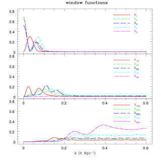
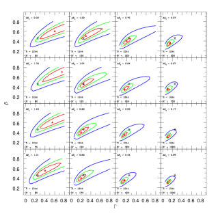
Figure 3: (left panel) The window functions in arbitrary units. The top panel shows the window functions associated with the five smallest eigenvalues. The center panel shows the window functions associated with five somewhat larger eigenvalues, while the bottom panel shows the window functions selected from the entire range of large eigenvalues. For each panel we show the eigenvalue rank for each window function. Figure 4: (right panel) Likelihood vs. $\Gamma$ and $\beta$ for the simulated catalog for different $N^{\prime}$, the number of moments kept; we also show the value of $\Delta\theta_{q}$. The panels show the maximum likelihood value (solid triangles) and the contours corresponding to $0.5,0.1$ and $0.01$ of the maximum values. The asterisk in each panel is the “true” value of $\Gamma=0.25$ and $\beta=0.457$ for the simulation. Increasing the number of modes $N^{\prime}$ improves the accuracy of the maximum likelihood values up to a point, but the inclusion of large eigenvalue modes that carry information mostly from nonlinear scales can skew the result away from the true value.

In Fig. 4 we show the results of the likelihood analysis on a typical catalog for various $N^{\prime}$. For reference, we also give the value of $\Delta\theta_{q}$ for each $N^{\prime}$. We see that in this case, inclusion of all of the information leads to the location of the maximum likelihood being skewed away from the true values. However, when higher order moments are discarded, the location of the maximum likelihood corresponds well with the true values. The fact that the discarding of higher order moments leads to a much better agreement between the maximum likelihood location and the true values is a good indication that our analysis method is effectively removing small–scale, nonlinear velocity information.

Although proper distance surveys present many challenges to cosmologists, they are quite well suited to the extraction of cosmological information provides they are handled with care and caution. In this conference I and my colleagues showed that with the right approaches we can extract interesting and important information and that techniques we have developed should be added to the cosmological toolbox.

References

References

- [1] Peebles, P.J.E. 1980 The Large Scale Structure of the Universe Princeton U. Press.
- [2] Shandarin, S. F., & Zel’dovich, Ya. B. 1989, Rev. Mod. Phys., 61, 185.
- [3] Feldman, H.A. & Frieman, J., Fry, J., Scoccimarro, R., 2001 Phys. Rev. Lett. 86, 1434.
- [4] Zel’dovich Ya.B. 1970, A&A, 5, 84
- [5] Watkins, R. & Feldman, H. A., 1995, ApJ Lett. 453 L72–76.
- [6] Feldman, H.A. & Watkins, R. 1998, ApJ 494 L129–132
- [7] Feldman, H. A. & Watkins, R., 1994, ApJ Lett. 430 L17–20.
- [8] Strauss, M., Cen, R., Ostriker, J. P., Postman, M. & Lauer, T. 1995 ApJ 444 507
- [9] Jacoby, G.H. et al. 1992, Publ. Astron. Soc. Pac. 104, 599.
- [10] Lauer, T. & Postman, M. 1994, ApJ 425 418.
- [11] Riess, A. G., Press, W. H., & Kirshner, R. P. 1995, ApJ, 438, L17
- [12] Jaffe, A. & Kaiser, N. 1995 ApJ 255 26
- [13] Croft, R. & Efstathiou, G., 1994, Potsdam Cosmology Workshop: astro–ph/9412024.
- [14] Bertschinger, E. & Dekel, A. 1989, ApJ Lett. 336, L5
- [15] Zaroubi, S., Hoffman, Y. & Dekel, A. ApJ 520, 413
- [16] Hudson, M., 2003, In this volume.
- [17] Hudson, M., Smith, R., Lucey, J., Schlegel, D. & Davies, R., 1999, ApJ Lett. L79.
- [18] Courteau, Strauss, & Willick, Eds., 2000, ASP Conf. Ser. 201, Cosmic Flows
- [19] S. Courteau , J. Willick , M. Strauss , D. Schlegel , & M Postman, 2000, ApJ 544, 636
- [20] Dale, D. A., Giovanelli, R. , Haynes, M. P., Campusano, L. E., Hardy, E. and Borgani, S., 1999, ApJ Lett. , 510, L11.
- [21] R. Saglia et al. , 1997, ApJ Supl. 109, 79.
- [22] Tonry, J. L. et al. , 2001, ApJ , 594, 1.
- [23] Riess, A. G., Press, W. H., & Kirshner, R. P. 1996 473 88
- [24] Juszkiewicz, R., Springel, V. & Durrer, R., 1999, ApJ , 518, L25
- [25] Ferreira, P. G., et al. , 1999, ApJ , 515, L1
- [26] Juszkiewicz, R., et al. , 2000, Sci, 287, 109
- [27] Feldman, H.A. et al. , 2003, ApJ Lett. 596 131L
- [28] Juszkiewicz, R., 2003, In this volume.
- [29] Willick, J. A., et al. , 1997, ApJ Supl. , 109, 333
- [30] da Costa, L. N., et al. , 1996, ApJ , 468, L5
- [31] da Costa, L. N., et al. , 2000, AJ , 120, 95
- [32] Karachentsev, I. D., et al. , 2000, Bull. Spec. Astrophys. Obs. N. Caucasus, 50, 5
- [33] Hamilton, A. J. S., & Tegmark, M. , 2002, MNRAS , 330, 506
- [34] Gaztañaga, E. & Juszkiewicz, R., 2001, ApJ , 558, L1
- [35] Kenney, J.F., & Keeping, E.S. 1954, Mathematics of statistics, Van Nostrand company.
- [36] Kendall, M. G. & Stuart, A. 1969 The advanced Theory of Statistics Vol. 2, Grifin.
- [37] Tegmark, M., Taylor, A.N. & Heavens, A.F., 1997, ApJ 480 22
- [38] Matsubara, T., Szalay, A.S. & Landy, S.D., 2000, ApJ 535:L1
- [39] Hoffman, Y. & Zaroubi, S., 2000, ApJ 535 L5
- [40] Hamilton, A., 2000 MNRAS 312 257
- [41] Hamilton, A. & Tegmark, M., 2000 MNRAS 312 285
- [42] Watkins, R., Feldman, H., Chambers, Gorman & Melott, 2002, ApJ 564 534
- [43] Feldman, H. A., Watkins, R., Melott, A. & Chambers, W., 2003, astro–ph/0304316
- [44] Feldman, Hume A., Watkins, R., Melott, A. & Chambers, W., 2003, In this volume.