IRAS 23385+6053: a candidate protostellar massive object

We present the results of a multi-line and continuum study towards the source IRAS 23385+6053 performed with the IRAM-30m telescope, the Plateau de Bure Interferometer, the Very Large Array Interferometer and the James Clerk Maxwell Telescope. We have obtained single-dish maps in the C¹⁸O (1–0), C¹⁷O (1–0) and (2–1) rotational lines, interferometric maps in the CH₃C₂H (13–12) line, NH₃ (1,1) and (2,2) inversion transitions, and single-pointing observations of the CH₃C₂H (6–5), (8–7) and (13–12) rotational lines. The new results confirm our earlier findings, namely that IRAS 23385+6053 is a good candidate high-mass protostellar object, precursor of an ultracompact Hii region. The source is roughly composed of two regions: a molecular core $\sim 0.03\div 0.04$ pc in size, with a temperature of $\sim 40$ K and an H₂ volume density of the order of 10⁷ cm^-3, and an extended halo of diameter $\leq$0.4 pc, with an average kinetic temperature of $\sim 15$ K and H₂ volume density of the order of 10⁵ cm^-3. The core temperature is much smaller than what is typically found in molecular cores of the same diameter surrounding massive ZAMS stars. From the continuum spectrum we deduce that the core luminosity is between 150 and $1.6\times 10^{4}L_{\odot}$, and we believe that the upper limit is near the “true” source luminosity. Moreover, by comparing the H₂ volume density obtained at different radii from the IRAS source, we find that the halo has a density profile of the type $n_{\rm H_{2}}\propto r^{-2.3}$. This suggests that the source is gravitationally unstable. The latter hypothesis is also supported by a low virial-to-gas mass ratio ($M_{\rm VIR}/M_{\rm gas}$ $\leq$0.3). Finally, we demonstrate that the temperature at the core surface is consistent with a core luminosity of $10^{3}\;L_{\odot}$ and conclude that we might be observing a protostar still accreting material from its parental cloud, whose mass at present is $\sim 6M_{\odot}$.

1 Introduction

The study of massive stars ($M\geq 10\leavevmode\nobreak\ M_{\odot}$) and their formation is important for a better understanding of the evolution and morphology of the Galaxy. However, up to now most progress has been done in the study of the formation of low-mass stars ($M\leq 1\leavevmode\nobreak\ M_{\odot}$). This is a consequence of the many observational problems which hinder the study of the high-mass star formation process: massive stars are more distant than low-mass ones, interact more strongly with their environment, have shorter evolutionary timescales and mainly form in clusters. Neverthless, recently a major observational effort has been made to identify the very earliest stages of their evolution. Successful results have been obtained searching for high-density and high-temperature tracers (e.g. NH₃ or CH₃CN) towards selected targets associated with regions of massive star formation, such as ultracompact Hii regions (Cesaroni et al. cesa94 (1994); Olmi et al. olmi96 (1996); Cesaroni et al. cesa98 (1998)), H₂O masers (Codella et al. code (1997); Plume et al. plume (1997); Beuther et al. 2002b ), and IRAS sources (Molinari et al. mol96 (1996); Beuther et al. 2002a ). Probably the most relevant finding of these studies is the detection of hot ($\ga$100 K), dense ($\ga 10^{7}$ cm^-3), molecular cores where high-mass stars have recently formed. It is believed that such “hot cores” (HCs, hereafter) represent the natal environment of O–B stars.

The next step in the search for very young massive stars is the detection of a genuine example of massive protostar. Molinari et al. (1998b ) suggested that the source IRAS 23385+6053 might be such an object.

IRAS 23385+6053 is one of a sample of IRAS sources selected in a long-standing project as a likely candidate massive protostar. The selection criteria used in this project are based on the IRAS colours (Palla et al. palla91 (1991)) and are aimed at identifying luminous (and hence likely massive) stellar objects in the earliest stages of their evolution. Observations of molecular tracers such as H₂O (Palla et al. palla91 (1991)) and NH₃ (Molinari et al. mol96 (1996)) have proven these objects to be associated with dense molecular gas. Additional observations in the continuum with the James Clerk Maxwell Telescope (JCMT, Molinari et al. mol00 (2000)) and the Very Large Array (VLA) (Molinari et al. 1998a ) have confirmed that a well defined sub-sample of these sources is embedded in dense dusty clumps (detected at mm and sub-mm wavelengths), and do not present any free-free emission, i.e. are undetected at centimeter wavelengths down to levels below that expected on the basis of their luminosity. The latter finding suggests that, although luminous (i.e. massive), the objects embedded in the clumps are still too young to develop an Hii region. Such a sample contains excellent targets to search for massive protostars.

Recently, Brand et al. (brand (2001)) have performed a single-dish multi-line study mapping a small number of these candidates in various molecular transitions, finding that they are associated with clumps that are larger, cooler, more massive and less turbulent than those associated with ultracompact Hii regions.

One of these sources, IRAS 23385+6053 (at a kinematic distance of $\sim 4.9$ kpc), was observed in more detail at different angular resolutions with the OVRO interferometer (Molinari et al. 1998b , mol02 (2002)) and the VLA (Molinari et al. mol02 (2002)). This object has also been observed with ISOCAM at 7 and 15 $\mu$m. The main findings of these first studies are the following:

• the source presents a compact molecular, dusty core with diameter $\sim$0.08 pc and mass $\sim$370 $M_{\odot}$, centered at $\alpha({\rm J2000})={\rm 23^{h}40^{m}}$54$\aas@@fstack{s}$5, $\delta({\rm J2000})=61^{\circ}10^{\prime}$28.^′′10. Hereafter, the name I23385 will be used to identify this core;

• the luminosity derived from the IRAS and JCMT continuum measurements for a distance of 4.9 kpc is $\sim$$1.6\leavevmode\nobreak\ 10^{4}\leavevmode\nobreak\ L_{\odot}$;

• no continuum emission from the core is detected at 2 and 6 cm with the VLA, down to $\sim$0.5 mJy beam^-1 (3$\sigma$);

• no continuum emission from the core is detected at 7 and 15 $\mu$m with ISOCAM down to $\sim$6 mJy beam^-1 (3$\sigma$);

• a faint, small ($\leq$0.1 pc) bipolar outflow with axis closely aligned with the line of sight has been seen in the SiO, HCO⁺, ¹³CO and CS line wings.

Molinari et al. (1998b ) concluded that I23385 is a good example of a luminous, young, deeply embedded (proto)stellar source.

Also, Molinari et al. (mol02 (2002)) discovered two extended Hii regions with the VLA at 3.6 cm which, however, do not coincide with I23385; rather they seem to overlap with a cluster of infrared sources detected with ISOCAM that surrounds the molecular peak. The infrared emission is coincident with a cluster of stars in near-infrared images (Molinari, priv. comm.). In this work, we discuss whether I23385 is a newly-born B0 star just arrived on the ZAMS or if it is a massive protostar still in the main accretion phase. For this purpose, the question we must answer is whether I23385 derives its luminosity primarly from hydrogen burning or from accretion. We believe that understanding the nature of I23385 can be improved by examining the physical parameters of the core, in particular by measuring the temperature of the associated core. In fact, in low-mass objects the temperature seems to be lower in the earlier evolutionary stages (Myers & Ladd 1993). By analogy, if high-mass ZAMS stars are found in “hot cores”, then high-mass protostars might lie inside colder cores. Furthermore, a detailed picture of the source, from small to large spatial scales, should be very useful to our purposes. We present here the results obtained from observations of the C¹⁸O and C¹⁷O (1–0), the C¹⁷O (2–1) and the CH₃C₂H (6–5), (8–7) and (13–12) lines using the IRAM-30m telescope and the Plateau de Bure Interferometer (PdBI). We also mapped the NH₃ (1,1) and (2,2) inversion lines with the VLA. In Sect. 2 we will describe the observations; in Sects. 3 and 4 we will present the observational results and derive the physical parameters of the source, respectively; in Sect. 5 we will discuss these results, and finally we will draw our conclusions in Sect. 6.

2 Observations and data reduction

2.1 IRAM-30m

The molecular transitions observed with the IRAM-30m telescope are listed in Table 1: here, we also give the frequencies, the half power beam width of the telescope, the total bandwidth used and the spectral resolution. The main beam brightness temperature, $T_{\rm MB}$, and the flux density, $F_{\nu}$, are related by the expression $F_{\nu}({\rm Jy})=4.9\;T_{\rm MB}(\rm K)$.

2.1.1 C¹⁸O and C¹⁷O

C¹⁸O and C¹⁷O data were obtained on September 5, 2000. We simultaneously used two 3 mm receivers centered at the frequencies of the C¹⁸O (1–0) and C¹⁷O (1–0), and two 1.3 mm receiver both centered at the frequency of the C¹⁷O (2–1) line to optimize the signal-to-noise ratio. For every line, three 3$\times$3 maps with grid spacings 6, 8 and 10^′′ and three 5$\times$5 point maps with the same grid spacing were made. All maps are centered at $\alpha({\rm J2000})={\rm 23^{h}40^{m}}$54$\aas@@fstack{s}$5, $\delta({\rm J2000})=61^{\circ}10^{\prime}$28.^′′10: this position corresponds to the sub-mm peak detected by Molinari et al. (mol00 (2000)). Map sampling allows us to cover a region $\sim 40$^′′ in size. Pointing and receiver alignment were regularly checked, and they were found to be accurate to within 2^′′. The data were calibrated with the “chopper wheel” technique (see Kutner & Ulich kutner (1981)). The integration time was 2 min per point in “wobbler-switching” mode, namely a nutating secondary reflector with a beam-throw of 240^′′ in azimuth and a phase duration of 2 s.

The system temperature was $\sim 250$ K at the frequency of the C¹⁷O (1–0) and C¹⁸O (1–0) lines, and it was $\sim 1000$ K in the C¹⁷O (2–1) line.

2.1.2 CH₃C₂H 

CH₃C₂H data were obtained on August 12, 1999. We simultaneously observed the (6–5), (8–7) and (13–12) rotational transitions in the 3 mm, 2 mm and 1.3 mm bands respectively. Only single-pointing observations were made. The data have been calibrated using the “chopper wheel” technique, and the observations were performed using the “wobbler-switching” mode. The system temperature was $\sim 120$ K at 3 mm, $\sim 260$ K at 2 mm and $\sim 350$ K at 1.3 mm.

Table 1: Transitions observed with the IRAM-30m telescope and the Plateau de Bure interferometer

Molecular	Rest freq.	HPBW (30m)	Band / Resolution (30m)	HPBW (PdBI)	Band / Resolution (PdBI)
transition	(GHz)	(′′)	(MHz)	(′′)	(MHz)
C18O (1–0)	109.782	23	70 / 0.078 ($\sim 0.2$ km s-1)	2.3$\times$1.94	16 / 0.156 ($\sim 0.4$ km s-1)
C17O (1–0)	112.359	22	70 / 0.078 ($\sim 0.2$ km s-1)	1.95$\times$1.45	17 / 0.156 ($\sim 0.4$ km s-1)
C17O (2–1)	224.714	11	70 / 0.078 ($\sim 0.1$ km s-1)	0.94$\times$0.75	25 / 0.312 ($\sim 0.4$ km s-1)
CH3C2H (6–5)	102.547$(^{*})$	24	70 / 0.078 ($\sim 0.2$ km s-1)	–	–
CH3C2H (8–7)	136.728$(^{*})$	18	70 / 0.078 ($\sim 0.2$ km s-1)	–	–
CH3C2H (13–12)	222.166$(^{*})$	11	140 / 0.078 ($\sim 0.1$ km s-1)	0.94$\times$0.76	33 / 0.312 ($\sim 0.4$ km s-1)

$(^{*})$ rest frequency of the $K=0$ transition

Figure 1: C¹⁸O and C¹⁷O spectra towards the central position in the maps, which is the peak of the sub-mm emission (Molinari et al. 2000). The dashed line indicates the main component arising from the source. The dotted line with red-shifted velocity shows the second component. In the C¹⁷O (1–0), the vertical lines under the spectrum indicate the position of the hyperfine components.

Figure 2: From top to bottom: CH₃C₂H (6–5), (8–7) and (13–12) IRAM-30m spectra towards the peak of the sub-mm emission (Molinari et al. 2000). The numbers under the spectra indicate the position of the different $K$ components. The $V_{\rm LSR}$ is relative to the line with $K=0$.

2.2 JCMT

An 850$\mu$m continuum image was taken on October 16 1998 with SCUBA at the JCMT (Holland et al. holland (1998)) towards the postion of the core I23385. The standard 64-points jiggle map observing mode was used, with a chop throw of 2 arcmin in the SE direction. Atmospheric conditions were not excellent, with $\tau_{225GHz}\sim$ 0.15. Telescope focus and pointing were checked using Uranus and the data were calibrated following standard recipes as in the SCUBA User Manual (SURF).

2.3 Plateau de Bure Interferometer

All transitions observed with the IRAM-30m telescope except for CH₃C₂H (6–5) and (8–7) have been observed also with the IRAM 5-element array at Plateau de Bure. The observations were carried out in November 1998 and April 1999 in the B and C configurations of the array. The antennae were equipped with 82–116 GHz and 210–245 GHz receivers operating simultaneously. These were tuned single side-band at 3 mm and double side-band at 1.3 mm resulting in typical system temperatures of 200 K (in the USB) and 1000 K (in the LSB) at 3 mm and 250 K (DSB) at 1.3 mm. The facility correlator was centred at 112.581 GHz in the USB at 3 mm and at 221.921 GHz in the LSB at 1.3 mm. The C¹⁸O(1–0) and C¹⁷O(1–0) lines were covered using two correlator units of 20 MHz bandwidth (with 256 channels); two 160 MHz units were suitably placed to obtain a continuum measurement at 3 mm. The C¹⁷O(2–1) and CH₃C₂H(13–12) $K$=0,1,2 transitions were observed with a 40 MHz bandwidth (256 channels), while the other $K$ lines were covered with 160 MHz bandwidths (64 channels), which were also used to obtain a continuum measurement at 1.3 mm. The effective spectral resolution is about twice the channel spacing (see “The New Correlator Description of the PdBI”, http://www.iram.fr).

Phase and amplitude calibration were obtained by regular observations (every 20 min) of nearby point sources (2200+420 and 0059+5808). The bandpass calibration was carried out on 3C454.3, while the absolute flux density scale was derived from MWC349, regulary monitored at IRAM. Continuum images were produced after averaging line-free channels and then subtracted from the line. The resulting maps were then cleaned and channel maps for the lines were produced. The synthesized beam sizes are listed in Table 1.

2.4 Very Large Array

The NRAO Very Large Array (VLA) ammonia observations were performed on August 8, 2000. The NH₃(1,1) and NH₃(2,2) inversion lines at 23.694496 and 23.722633 GHz, respectively, were simultaneously observed with spectral resolutions of 1.2 and 4.9 km s^-1 respectively. The array was used in its most compact configuration (D), offering baselines from 35 m to 1 km. The flux density scale was established by observing 3C286 and 3C147; the uncertainty is expected to be less than 15%. Gain calibration was ensured by frequent observations of the point source J0102$+$584, with a measured flux density at the time of the observations of 3.4 Jy. The same calibrator was also used for bandpass correction.

The data were edited and calibrated using the Astronomical Image Processing System (AIPS) following standard procedures. Imaging and deconvolution was performed using the IMAGR task and naturally weighting the visibilities. The resulting synthesised beam FWHM is 4.0${}^{\prime\prime}\times 3.7^{\prime\prime}$ with position angle $-50^{\circ}$, and the noise level in each channel is 4 mJy beam^-1 and 3 mJy beam^-1 for the NH₃(1,1) and NH₃(2,2) data respectively.

2.5 Data reduction and fitting procedures

The reduction of the IRAM-30m telescope and PdBI data has been carried out with the GAG-software developed at IRAM and the Observatoire de Grenoble. In the next subsections we briefly outline the fitting procedures adopted to analyze the CH₃C₂H and NH₃ spectra.

2.5.1 CH₃C₂H fitting procedure

CH₃C₂H is a symmetric-top molecule with small dipole moment ($\mu=0.75$ Debye). Its rotational levels are described by two quantum numbers: $J$, associated with the total angular momentum, and $K$, its projection on the symmetry axis. Such a structure entails that for each $J+1\rightarrow J$ radiative transition, $J+1$ lines with $K\leq J$ can be seen (for a detailed description see Townes & Schawlow townes (1975)). In our observations the bandwidth covers all components for the (6–5) and (8–7) transitions, and up to the $K=10$ component for the (13–12) line. However, we detected only lines up to $K=3$.

In order to compute the line parameters, we have performed Gaussian fits to the observed spectra assuming that all the $K$ components of each $J+1\rightarrow J$ transition arise from the same gas. Hence, they have the same LSR velocity and line width. Then, in the fit procedure we fixed the line separation in each spectrum to the laboratory value and we assumed the line widths to be identical. In Sect. 4 we will use the line intensities derived from this procedure to estimate the kinetic temperature of the emitting gas.

2.5.2 NH₃ fitting procedure

The NH₃ (1,1) and (2,2) inversion lines show hyperfine structure (see i.e. Townes & Schawlow townes (1975)). To take into account this structure, we fitted the lines using METHOD NH₃(1,1) and METHOD NH₃(2,2) of the CLASS program. In this case the fit to the NH₃ lines is performed assuming that all components have equal excitation temperatures, that the line separation is fixed at the laboratory value and that the linewidths are identical. This method also gives an estimate of the total optical depth of the lines using the intensity ratio between the different hyperfine components.

3 Results

3.1 IRAM-30m observations

3.1.1 C¹⁸O and C¹⁷O spectra

In Fig. 1 we show the C¹⁸O and C¹⁷O spectra taken at the central position in the maps, corresponding to the peak of the sub-mm emission detected by Molinari et al. (mol00 (2000)). Single-pointing spectra of the CH₃C₂H (6–5), (8–7) and (13–12) lines are shown in Fig. 2. The C¹⁸O (1–0) and C¹⁷O (1–0) spectra towards the central position clearly indicate the presence of two velocity components, centered at $\sim-50.5$ km s^-1and at $\sim-47.8$ km s^-1, respectively (see Fig. 1). The component with higher velocity appears very strong especially in the C¹⁸O (1–0) spectrum. We have fitted the two components with Gaussians. In particular, the C¹⁷O (1–0) line has hyperfine structure: thus, we have performed Gaussian fits taking into account this structure by using METHOD HFS of the CLASS program. This procedure also gives an estimate of the line optical depth: we will discuss this point in Sect. 3.1.3. The line parameters of the two components at the peak position are given in Table 2. Peak velocity ($V_{\rm lsr}$), full width half maximum ($\Delta v$) and integrated intensity of the line ($\int T_{\rm MB}{\rm d}v$) are given in Cols. 3, 4 and 5, respectively. In Col. 2 we also give the 1$\sigma$ rms of the spectra. In the CH₃C₂H observations only the lower velocity component is seen. For these lines, we have performed Gaussian fits as explained in Sect. 2.5. The results are given in Table 3.

3.1.2 C¹⁸O and C¹⁷O integrated intensity maps

Maps of the spectral component at $-47.8$ km s^-1 show that the C¹⁸O (1–0) (Fig. 3) and the C¹⁷O (2–1) lines peak at (0^′′,$-15$^′′) from the central position of I23385, suggesting that this emission is unrelated to this source. The presence of a secondary source to the South was already found by Molinari et al. (1998b ) in the HCO⁺(1–0) line. Only the component centered at $-50.5$ km s^-1 represents the emission arising from I23385: hereafter we shall refer to this as the “main” component. The secondary component, centered at $-47.8$ km s^-1, will not be discussed further.

Table 2: Line parameters of CO isotopomers at the peak position (IRAM-30m observations). All line parameters have been obtained from a two-Gaussian fit, except for the C¹⁷O (1–0) line, for which we have used METHOD HFS of the CLASS program to take into account the hyperfine structure (see text).

Line	rms	$V_{\rm lsr}$	$\Delta v_{1/2}$	$\int T_{\rm MB}{\rm d}v$
	(K)	(km s-1 )	(km s-1 )	(K km s-1 )
C18O (1–0)	0.065	$-50.0$	2.38	3.73
		$-47.8$	1.20	2.59
C17O (1–0)	0.064	$-49.9$	2.08	1.18
		$-47.5$	1.12	0.41
C17O (2–1)	0.18	$-49.8$	2.93	5.06
		$-47.3$	0.90	0.69

Table 3: CH₃C₂H line parameters (IRAM-30m observations)

Line	rms	$v_{\rm LSR}$	$\Delta v_{1/2}$	$\int T_{\rm MB}{\rm d}v$ (K km s-1)
	(K)	(km s-1)	(km s-1)	$K=0$	1	2	3
CH3C2H (6–5)	0.011	$-50.3$	2.48	0.37	0.29	0.13	0.07
CH3C2H (8–7)	0.024	$-50.5$	2.64	0.41	0.40	0.22	0.13
CH3C2H(13–12)	0.032	$-50.5$	2.57	0.75	0.71	0.41	0.30

The integrated intensity maps of the main component are shown in Figs. 3 and 4. We do not show the C¹⁷O (1–0) integrated map because the line is faint over the whole map (S/N$\leq 3\sigma$ in many points). The first clear result is that the emission looks quite flat and without an obvious peak towards I23385. This is especially evident in the C¹⁷O map. Also, in the C¹⁸O (1–0) and C¹⁷O (2–1) maps, the half maximum power contour is elongated in the N-S direction: this could be due to the presence of the secondary component in the spectra. In fact, it is difficult to separate the two components, especially in the southern part of the map where the overlap of the two lines is more pronounced. In an attempt to derive the size of the emtting region in each line, we have estimated the angular diameter considering only the northern part of the maps (that with positive offset in $\delta$), which is less affected by the secondary component: we find an average diameter of the emitting region $\sim 22$^′′ for the C¹⁸O (1–0) line, and $\sim 18$^′′ for the C¹⁷O (2–1) line. After correcting for the beam size (see Table 1), one finds a deconvolved angular diameter of $\sim 18$^′′ (corresponding to $\sim 0.45$ pc) for the C¹⁸O (1–0) line and of $\sim 15$^′′ ($\sim 0.30$ pc) for the C¹⁷O (2–1) line.

In conclusion, from the 30-m maps of I23385 in the C¹⁸O and C¹⁷O lines, one cannot see an intensity peak towards the nominal position of the core, which instead is clearly seen by Molinari et al. (1998b ) in different molecular transitions, as well as in our PdBI maps in the same lines, as shown in Sect. 3.3. We will further discuss this point in Sect. 5.2.

3.1.3 Optical depth of the lines

The availability of two rotational transitions of the same molecular species (namely C¹⁷O (1–0) and (2–1)) allows us to derive a map of the kinetic temperature, as we will explain in Sect. 4.3. However, this requires knowledge of the optical depth of such lines. Since we have also observed the C¹⁸O (1–0) line, it is possible to estimate the opacity of the C¹⁷O (1–0) line from the ratio of two spectra, assuming equal temperatures and beam filling factors, and an abundance ratio of 3.7 for ¹⁸O/¹⁷O (see Penzias penzias (1981), Wilson & Rood wilson (1994)). We find an intensity ratio typically between 3 and 4, with a mean value of $\sim 3.5$, which implies that the C¹⁷O (1–0) line is optically thin.

For C¹⁷O, it is possible to derive the optical depth from the measure of the relative intensities of the hyperfine components. Unfortunately, in our spectra we are not able to resolve the hyperfine structure, hence the optical depth derived in this way is not reliable. Concerning the C¹⁷O (2–1) line, we cannot measure the optical depth directly from our observations. However, in LTE conditions, one can demonstrate that up to temperatures as high as $\sim 40$ K, the optical depth of the (2–1) line is $\leq$ 3 times that of the (1–0) line. Since the maximum value of the opacity of the (1–0) line derived from the line ratio is $\tau\sim 0.18$, the (2–1) line must have an optical depth less than $\sim 0.5$. Thus, when in Sect. 4.3 we will derive the kinetic temperature from the ratio between the C¹⁷O (2–1) and (1–0) lines, we will assume that the lines are optically thin.

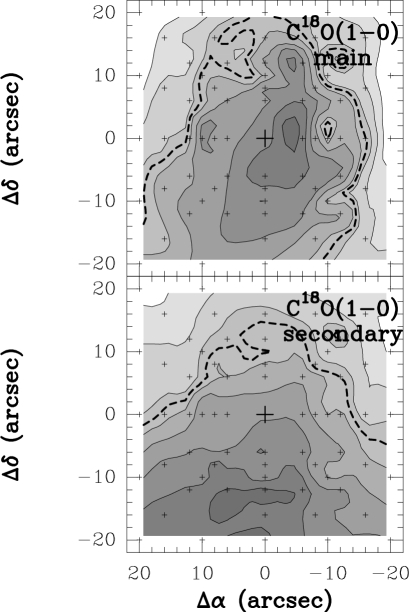
Figure 3: Top panel: IRAM-30m map of the main component of the C¹⁸O (1–0) line obtained integrating between $-52.5$ and $-49.0$ km s^-1. Contour levels go from $\sim 1.5$ K km s^-1 (corresponding to $\sim 3\sigma$), to the maximum value of $\sim$4 K km s^-1 in steps of 0.5 K km s^-1 ($\sim 1\sigma$). The thick, dashed contour indicates the half maximum power contour. Bottom panel: same as Top for the secondary component of the C¹⁸O (1–0) line, integrated between $-49.0$ and $-45.0$ km s^-1. Contour levels range from 1 K km s^-1 ($\sim 3\sigma$) to 3.3 K km s^-1 in steps of 0.3 K km s^-1 ($\sim 1\sigma$).

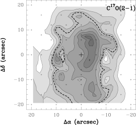
Figure 4: Same as Fig. 3 for the main component of the C¹⁷O (2–1) line, integrated between $-52.5$ and $-49.0$ km s^-1. Contour levels go from $\sim 1$K km s^-1 ($\sim 3\sigma$ level), to 3.3 K km s^-1 in steps of $1\sigma$.

3.2 JCMT observations

I23385 has been mapped in the sub-mm continuum at 850$\mu$m with SCUBA, with an angular resolution of 15 ^′′ (Fig. 5). The intensity profile presents an unresolved compact central peak, and an extended halo which surrounds the peak up to $\sim 100$ ^′′. The figure also shows the integrated emission of the main component of the C¹⁸O (1–0) line (upper panel of Fig. 3). We can see that there is a reasonable match between the 850 $\mu$m emitting region and that traced by the C¹⁸O (1–0) line, although the corresponding peaks are not coincident.

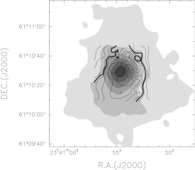
Figure 5: SCUBA map of IRAS 23385+6053 at 850 $\mu$m (grey scale). Levels range from 0.3 (3$\sigma$) to 1.9 by 0.2 Jy beam^-1. The solid contours represent the C¹⁸O (1–0) map (main component) obtained with the IRAM-30m telescope (Fig. 3), with the thick line corresponding to the contour at half maximum.

3.3 Plateau de Bure observations

We present here the results of molecular line and millimeter continuum observations carried out with the Plateau de Bure Interferometer.

3.3.1 Molecular lines

All molecular transitions observed with the IRAM-30m telescope have been also imaged with the PdBI, with the exception of the CH₃C₂H (6–5) and (8–7) lines. In Fig. 6 we show the maps obtained integrating the emission under the C¹⁸O (1–0), C¹⁷O (2–1) and CH₃C₂H (13–12) lines. The secondary component is not detected, except perhaps in C¹⁸O (1–0), in which the shape of the red wing of the line might be affected by the secondary component. This is likely due to the fact that the secondary component is more extended, thus its emission has been resolved out.

We do not show the C¹⁷O (1–0) map because this is very noisy, and the signal is undetected up to a $3\sigma$ level of $\sim 36$ mJy beam^-1. The C¹⁸O (1–0), C¹⁷O (2–1) and CH₃C₂H (13–12) emission is detected with a good signal-to-noise ratio. We can clearly see the presence of a central compact core coincident with I23385. In the C¹⁷O (2–1) and CH₃C₂H (13–12) lines, the source shows a complex morphology, while it looks more simple in the C¹⁸O (1–0) line. This is consistent with the different angular resolution: at 1.3 mm the beam size is $\sim 2$ times smaller, allowing us to better resolve the core structure. In particular, it can be noted that the C¹⁷O (2–1) emission is marginally depressed at the peak position of the continuum and the CH₃C₂H (13–12) line. This might be suggestive of CO depletion in the inner region of the core (see discussion in Sect. 5.2).

We have estimated the diameters of the emitting regions from the half maximum power contours shown in Fig. 6: if we assume the source to be Gaussian, we can derive the angular diameter after beam deconvolution, as given in Col. 2 of Table 5.

In Fig. 7 spectra of the C¹⁸O (1–0), C¹⁷O (1–0) and (2–1) and CH₃C₂H (13–12) lines are shown, that have been obtained integrating the emission arising within the $4\sigma$ level inferred from the maps of Fig. 6. The availability of IRAM-30m spectra allows a comparison between interferometric and single-dish data. This comparison is also shown in Fig. 7, where the single-dish spectra have been resampled with the same resolution in velocity as the PdBI spectra, namely $\sim 0.4$ km s^-1. The superposition of the spectra clearly demonstrates that a large fraction of the extended emission is filtered out by the interferometer. This is especially evident in the C¹⁸O (1–0) line, for which the flux measured with the PdBI is $\sim 11$ times less than those obtained with the IRAM-30m telescope. This is also true for the C¹⁷O (2–1) line, for which the intensity ratio is $\sim 10$. In the CH₃C₂H (13–12) transition this effect is smaller as the single-dish flux is $\sim 3$ times larger. As noted earlier, the secondary component is resolved out in the PdBI spectra.

Looking at the C¹⁷O (2–1) spectrum of Fig. 7, the line profile seen by the interferometer seems to peak at a slightly blue-shifted velocity with respect to the 30-m spectrum. We believe that this is due to the fact that the S/N ratio is poor in the PdBI spectrum, hence the peak velocity, and the other line parameters, are affected by large uncertainties. In fact, the offest observed ($\sim 0.5$ km s^-1) lies within the $3\sigma$ uncertainty on the line peak velocity ($\sim 0.45$ km s^-1) obtained from a Gaussian fit.

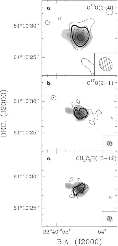
Figure 6: Maps obtained with the PdBI. a: C¹⁸O(1–0) map integrated over the velocity range ($-49$,$-52$) km s^-1. Contour levels range from 0.05 ($\sim 3\sigma$) to 0.14 by 0.02 Jy beam^-1. The thick contour indicates the half maximum power contour. The spectral rms is $\sim 0.014$ Jy beam^-1. The grey-scale image shows the 3 mm continuum emission, ranging from $\sim 1.9$ ($\sim 4\sigma$) to $7.4$ by 0.8 mJy beam^-1. The ellipse at the bottom right represents the synthesised beam. b: same as a for the C¹⁷O (2–1) line. The map has been integrated over ($-47$,$-52$) km s^-1. Contour levels range from 0.03 to 0.09 by 0.015 Jy beam^-1. The grey-scale image represents the 1.3 mm continuum emission, whose countour levels range from 6 to 24 by 2.5 mJy beam^-1. The spectral rms is $\sim 0.012$ Jy beam^-1. c: same as b for the CH₃C₂H (13–12) line, integrated under the K=0 and 1 lines. Contour levels range from 0.03 to 0.1 by 0.01 Jy beam^-1. The spectral rms is $\sim 0.013$ Jy beam^-1

Figure 7: Flux density comparison between IRAM single-dish (dashed line) spectra and Plateau-de-Bure interferometric spectra (solid line). The interferometric flux densities have been multiplied by a factor of 10 for the CO isotopomers, and by a factor of 3 for the CH₃C₂H lines. The velocity of the CH₃C₂H spectrum is computed with respect to the frequency of the line with $K=0$.

3.3.2 Millimeter continuum

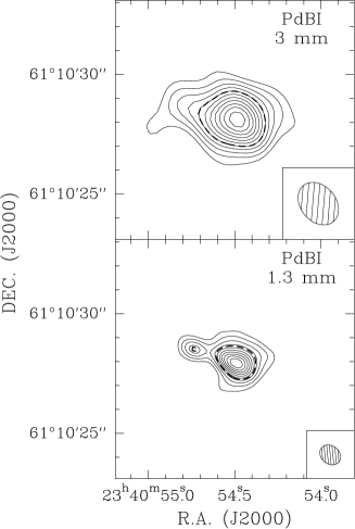
Figure 8: Top panel: map of the 3 mm continuum emission. The rms level is $\sim 0.6$ mJy beam^-1 and the signal-to-noise ratio is $\sim 15$. Contour levels range from 1.6 to 7.8 by 0.6 mJy beam^-1. The thick, dashed contour represents the half maximum power contour. Bottom panel:same as top for 1 mm continuum emission. The rms is $\sim 2$ mJy beam^-1 at 1.3 mm and the signal-to-noise ratio is $\sim$14. Contour levels range from 6 to 24 by 2 mJy beam^-1. The ellipses in the bottom right are the synthesized beams.

With the PdBI we detect a compact central core, as can be seen from Fig. 8, where we show the 3 mm and 1.3 mm continuum maps. The 3 mm map shows a compact core with an elongated shape along the E-W direction. This shape is better resolved at 1.3 mm, revealing a secondary faint peak of emission offset by $\sim+2$ ^′′ in R.A. from the main peak. This secondary peak is not detected in any of the molecular tracers. The angular diameters are 1.5^′′ and 1.1^′′ at 3 mm and 1.3 mm, respectively. Measured flux densities $F_{\nu}$ are 0.0124 and 0.148 Jy at 3 and 1.3 mm, respectively, obtained by integrating over the solid angle down to the 3$\sigma$ level. The flux density of the secondary source at 1.3 mm is $\sim 5\%$ of the total, namely 0.008 Jy.

We can compare the continuum flux density measured with the PdBI and with SCUBA, to estimate the amount of the flux density filtered out by the interferometer. Using a spectral index for the dust emissivity of 4 (see Sect. 4.1), we have extrapolated the flux density observed at 850 $\mu$m with SCUBA, to 1.3 mm. This has been smoothed to an angular resolution of $\sim 22$^′′, corresponding to the primary beam of the PdBI at 1.3 mm. The flux density measured in this map towards the core I23385 is $\sim 0.28$ Jy. We estimate in $\sim 0.11$ Jy the flux density to arise from the halo: this is filtered out by the interferometer, and thus the flux density that we should observe with the PdBI is $\sim 0.17$ Jy. Taking into account the uncertainties that affect our measurements (in particular the combined calibration errors of both SCUBA and PdBI, which are at least of the order of 30$\%$), the 0.15 Jy observed at 1.3 mm with PdBI is consistent with what is expected. Thus, within the errors, it is plausible that with the PdBI we observe all the continuum flux arising from the core I23385.

3.4 Very Large Array NH₃ maps

With the VLA, we have mapped the NH₃ (1,1) and (2,2) inversion transitions. The corresponding maps and integrated spectra are shown in Fig. 9. In both maps, the NH₃ emission is superimposed on the C¹⁸O (1–0) map. As for the CO isotopomers observed with the IRAM-30m telescope, the emission does not peak towards the position of the core detected at 3 mm and 1.3 mm with the PdBI. Although the signal-to-noise ratio is poor in both maps (see Fig. 9), one can see that the emission arises from a “clumpy” structure, and it peaks at $\sim 5$^′′ ($\sim 0.12$ pc) from the core position. In Sect. 5.2 we will discuss this result by comparing the NH₃ maps with those obtained in the other tracers. Comparison between Effelsberg-100m (Molinari et al. mol96 (1996)) and VLA observations are shown in Fig. 10. For the main component (centered at $-50.5$ km s^-1), with the VLA we lose about the 50$\%$ of the total flux density seen with the single-dish telescope; for the NH₃ (1,1) line, this occurs for all the hyperfine lines. Finally, we completely resolve out the secondary component (centered at $-47.8$ km s^-1) as in the other molecular tracers observed with the PdBI .

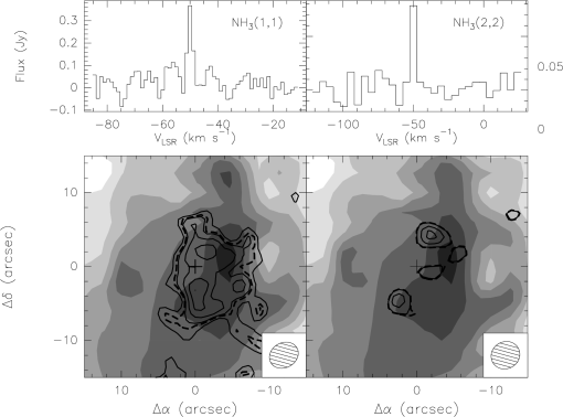
Figure 9: Left panel: NH₃(1,1) integrated map over the velocity range ($-48$, $-52$) km s^-1 . Contour levels range from 0.012 ($\sim 3\sigma$) to 0.024 by 0.004 Jy beam^-1. The channel spacing of the integrated spectrum (shown over the map) is $\sim 1.13$ km s^-1. The grey-scale represents the C¹⁸O (1–0) main line emission (Fig. 3). The cross indicates the core position detected with the PdBI. Right panel: same as Left for NH₃(2,2). Contour levels range from 0.012 to 0.025 by 0.004 Jy beam^-1. The channel spacing is $\sim 4.9$ km s^-1. The ellipses in the bottom-right represent the VLA synthesised beam.

Figure 10: Flux density comparison between Effelsberg-100m (dashed line) and VLA (solid line) spectra of the NH₃(1,1) and (2,2) lines. VLA fluxes have been multiplied by a factor of 2. The thick vertical lines under the NH₃(1,1) spectrum indicate the position of the two components. The Effelsberg spectra have been resampled to the channel spacing of the VLA spectra.

4 Derivation of physical parameters

Our goal is to investigate the hypothesis of Molinari et al. (1998b ), namely that I23385 is a high-mass protostellar object, by examining the physical parameters of the core. First, we will analyze the continuum spectral energy distribution (SED). Then, from the PdBI map of the CH₃C₂H (13–12) line, we will compute the core temperature; finally, from continuum and line emission we will obtain the mass and the H₂ volume density of the core.

4.1 Continuum SED and source luminosity

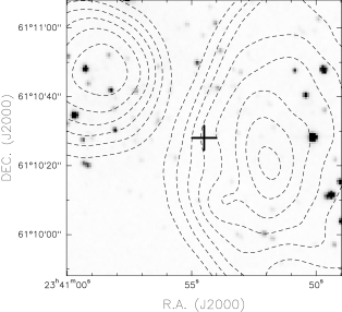
Figure 11: Image: IRAS 23385+6053 observed at 2 $\mu$m with the IRCAM of the Palomar telescope in the Ks band (Molinari priv. comm.), which shows the cluster of stars around the core I23385 (indicated by the cross at map center). The dashed contours represent the emission of the two extended radio sources detected at 3.6 cm with the VLA: contour levels range between 0.3 and 3 by 0.3 mJy beam^-1 (Molinari et al. mol02 (2002)).

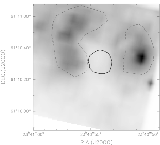
Figure 12: Image of IRAS 23385+6053 at 15 $\mu$m obtained with ISOCAM (Molinari et al. 1998b ). The thick polygon represents the 3$\sigma$ level of the HCO⁺ (1–0) line, and it identifies the core region. The dashed polygons indicate the two clusters of stars which lie around I23385, called “ring” in the text.

Figure 13: Continuum SED of I23385. Open hexagons and stars indicate MSX and ISOCAM flux densities respectively measured integrating over the “ring” region of Fig. 12. The filled triangle represents the SCUBA measurement. Filled squares, open squares, filled circles and open circles indicate respectively IRAS, JCMT, PdBI and OVRO data (see also Fig. 2 of Molinari et al. 1998b ). The arrows on the bottom left and bottom right respectively indicate the ISOCAM and VLA upper limits ($3\sigma$ level) of the core flux density. The solid line represents a grey-body fit, with dust temperature $T=40$ K and dust absorption coefficient $\beta\propto\nu^{1.9}$, while the dotted line is a grey-body fit with the same $\beta$ and $T=15$ K. The dashed line corresponds to a power-law extrapolation of the flux density arising from the “ring” region.

In discussing the continuum SED, it is important to distinguish between two “sub-regions”:

• the core I23385;

• a stellar and diffuse emission from a cluster surrounding the core (see Fig. 11).

The cluster is detected as a patchy “ring” at FIR wavelengths with ISOCAM (Fig. 12) and it seems to overlap with two extended sources detected at 3.6 cm with the VLA. From the radio flux Molinari et al. (mol02 (2002)) have estimated the spectral type of the ionizing stars to be B0.5.

In Fig. 13 the continuum SED of I23385 is shown. With respect to Fig. 2 of Molinari et al. (1998b ), Fig. 13 contains more data, namely PdBI, IRAS, JCMT, OVRO, ISOCAM and MSX . Since no 7 and 15 $\mu$m emission is detected with ISOCAM towards the source, we take the $3\sigma$ level as an upper limit at these wavelengths. The same was done for the VLA measurements at centimeter wavelengths.

We performed a grey-body fit to the continuum SED of Fig. 13 (solid line). The resulting bolometric luminosity is the same as in Molinari et al. (1998b ), namely $L\sim 1.6\;10^{4}\;L_{\odot}$. The slope of the millimetric part of the spectrum is fitted assuming a dust opacity $k_{\nu}=k_{230{\rm GHz}}(\nu/230(\rm GHz))^{\beta}$, where $k_{230{\rm GHz}}=0.005{\rm\;cm^{2}g^{-1}}$, which assumes a gas-to-dust mass ratio of 100 (see Preibisch et al. preib (1993)). The best fit is obtained for $F_{\nu}\propto\nu^{3.9}$. Therefore, the best fit opacity index is $\beta\simeq 1.9$. The other best fit parameters are: source temperature of 40 K, diameter of 8^′′and a mass of $\sim 400M_{\odot}$. Since most of the luminosity is due to the IRAS 60 and 100 $\mu$m flux densities, it is important to assertain the origin of the IRAS flux densities. In fact, the IRAS beam is much larger than the source diameter ($\sim 2$ arcmin at 100 $\mu$m), thus the IRAS flux densities may arise both from I23385 and from the cluster of stars surrounding it (the “ring” in the 15 $\mu$m ISOCAM map of Fig. 12). Hence, the source luminosity estimated before ($L\sim 1.6\;10^{4}\;{\rm L_{\odot}}$) is to be regarded as an upper limit for the luminosity of I23385. However, we know from the JCMT and interferometric maps that the flux densities at 850 $\mu$m and at longer wavelenghts certainly come from I23385. Thus, we performed a grey-body fit using only these data (dotted line of Fig. 13): the corresponding grey-body fit gives a luminosity of $\sim 150\;L_{\odot}$ which represents a lower limit. The two limits thus obtained are very different, but we believe that the source luminosity is closer to the upper limit. In fact, the MSX image at 21 $\mu$m shows that the emission at this wavelength arises from the “ring”, hence very likely this region is also responsible for the 25 $\mu$m emission. However, as already discussed by Molinari et al. (1998b ), it is unlikely that the “ring” contributes significantly to the IRAS flux densities at 60 and 100 $\mu$m, because even a power-law extrapolation of the spectrum of the extended region (dashed line in Fig. 13) gives flux densities at 60 and 100 $\mu$m much lower (a factor of $\sim 10$) than the values observed. We conclude that most of the emission at 60 and 100 $\mu$m is due to I23385, and therefore a luminosity of $\sim 10^{4}\;L_{\odot}$ is not very far from the real value. We will further discuss this point in Sect. 5.3, on the basis of our CH₃C₂H observations.

It is also worth noting that the 1.3 mm flux density measured with the PdBI is $\sim 3$ times less than the value measured with the JCMT at the same wavelength. In fact, as explained in Sect. 3.3.2, with the interferometer we observe approximately all the flux density arising from the compact core, but we miss that coming from the extended halo, which we do detect with the JCMT. Finally, it is unlikely that the source associated with the secondary peak detected in the 1.3 mm map contributes significantly to the total observed luminosity, because its 1.3 mm flux density is only 5$\%$ of that from the main core.

4.2 Kinetic temperature and column density from CH₃C₂H rotation diagrams

From the CH₃C₂H (13–12) spectra of Figs. 2 and 7 we derive the kinetic temperature and the total column density of the molecule by means of the Boltzmann diagrams method (see e.g. Fontani et al. fonta (2002)). The fundamental assumption of the method is the local thermodynamic equilibrium (LTE) condition of the gas. Such an assumption is believed to work very well for CH₃C₂H because of its low dipole moment (see Bergin et al. bergin (1994)). Under the further assumption of optically thin emission, the column density $N_{\rm i}$ of the upper level $i$ of each transition is proportional to the integrated intensity of the line.

In Fig. 14 Boltzmann diagrams are shown: the straight lines represent least square fits to the data, and the kinetic temperature and the column density are related to the slope and the intercepta, respectively. The interferometric data yield $T_{\rm k}\simeq 42$ K and $N_{\rm tot}\simeq 4\;10^{14}$ cm^-2 for the core. It is evident that such temperature is well below that of a HC. In a recent paper, Thompson & Macdonald (thompson (2003)) have observed rotational transitions of the CH₃OH molecule towards IRAS 23385+6053, from which they derive that the kinetic temperature is likely to be smaller than 50 K, and therefore it is unlikely that IRAS 23385+6053 might contain a HC. Our study strongly supports this idea and give a much more accurate temperature estimate of the core.

With the IRAM-30m data we obtain $T_{\rm k}\simeq 34$ K and $N_{\rm tot}\simeq 5\;10^{15}$ cm^-2. In this case, the column densities $N_{\rm i}$ have been corrected for the beam filling factor. For this purpose, an estimate of the CH₃C₂H emitting region is needed. Unfortunately, we have no direct estimate because no CH₃C₂H single-dish maps are available. However, we can use the source size estimated from the SCUBA map, given in Sect. 4.5.

The previous results are summarised in Table 4. The errors on $T_{\rm k}$ and $N_{\rm tot}$ have been computed in two different ways: for the single-dish data we must take into account the calibration error. This error affects simultaneously each line in the same bandwidth. Hence, in the diagrams, the effect of this error is to shift the points in the same bandwidth (e.g. the (6–5) lines) by the same quantity. This error is $\sim 10\%$ for the (6–5) lines and $\sim 20\%$ for the (8–7) and (13–12). Hence, in order to compute the uncertainties on $T_{\rm k}$ and $N_{\rm tot}$, we have varied the values of $N_{\rm i}$ by 10% simultaneously for all the (6–5) K components, and by 20% for the (8–7) and (13–12). These variations have been made in different directions. The uncertainties in Table 4 are the maximum difference between the values thus obtained and the nominal ones. For the PdBI estimates, we have data of a single band, and the calibration error does not affect $T_{\rm k}$ but only $N_{\rm tot}$.

Let us now discuss the two basic assumptions of the method, i.e. optically thin emission and LTE conditions of the gas. The LTE assumption holds very well when the H₂ density is greater than a critical value (see e.g. Spitzer spitzer (1978)). For the observed transitions the maximum critical density is $\sim 10^{5}$ cm^-3, and we shall see in Sect. 4.5 that the inferred H₂ density is above this value, justifying the assumption of LTE conditions. Concerning the optical depth of the lines, the excellent agreement between the data and the linear fit of Fig. 14 strongly supports the assumption of optically thin lines. In fact, large optical depths are expected to affect mainly the transitions with lower excitation. Hence we should have a flattening of the Boltzmann diagram at lower energies, which is not seen in Fig. 14.

4.3 Physical parameters from CO isotopomers

In the previous section we have computed the kinetic temperature of the source from the CH₃C₂H lines. We can also estimate the temperature by means of the C¹⁷O lines observed with the IRAM-30m telescope. Using a source size of $15$^′′, found in Sect. 3.1.2 from the C¹⁷O (2–1) map, we have derived the beam-averaged brightness temperatures for the C¹⁷O (1–0) and (2–1) lines. Then, from the integrated line intensities, and assuming optically thin lines and LTE conditions, we find a “Boltzmann relationship” between the total column density of the upper level of each transition and the corresponding rotational energy, as discussed above for the CH₃C₂H lines. We have done this for each point of the C¹⁷O maps in which the C¹⁷O (1–0) line is stronger than the $3\sigma$ level. The resulting average kinetic temperature is $\sim 15$ K. It is important to stress that in deriving the kinetic temperature from C¹⁷O line ratios we have assumed LTE conditions. Statistical equilibrium calculations (see Wyrowski wyrowski (1997)) show that this assumption holds if $n_{\rm H_{2}}\geq 10^{5}$ cm^-3. Otherwise, the temperature estimated in this way is to be regarded as a lower limit. Since we obtain $n_{\rm H_{2}}\sim 10^{5}$ cm^-3 over the whole map, we conclude that the LTE assumption is satisfied in our case.

We obtain a total column density ranging from $9\;10^{14}$ to $7\;10^{15}$ cm^-2: the C¹⁷O total column density given in Table 4, namely $4\;10^{15}$ cm^-2, is the mean value over the map.

4.4 Physical parameters from NH₃ (1,1) and (2,2)

The NH₃ emission seen with the VLA arises from a region whose diameter is “intermediate” between that of the core I23385 and that of the C¹⁷O and C¹⁸O total emitting region seen with the IRAM-30m telescope. The emission peak does not coincide with the continuum nor with the C¹⁸O (1–0) line. The NH₃ (1,1) hyperfine structure allows us to estimate the optical depth as explained in Sect. 2.5: we obtain $\tau\ll 1$ for this line. For the (2,2), we have no direct estimates, but we can reasonably assume that for temperatures between $\sim 10$ and $\sim 40$ K, under LTE conditions, the (2,2) line is also optically thin. The temperature and column density can be derived following the method by Ungerechts et al. (ung (1986)). We obtain a temperature of $\sim 26$ K and a total column density of 6 $10^{15}$ cm^-2. We have assumed equal linewidth and beam filling factor for both transitions. The results are given in Table 4.

4.5 Mass and density estimate

The grey-body fit to the spectrum of Fig. 13 is obtained for a dust temperature of 40 K, a dust opacity $k_{\nu}\propto\nu^{1.9}$, an average source diameter of 8^′′, ($\sim 0.2$ pc), and a mass of $\sim 400$ M_⊙.

It is also useful to derive the mass of the core seen with the PdBI. From the 3 mm continuum flux density, using the core temperature deduced from the CH₃C₂H lines (namely $T=42$ K), $k_{\nu}\propto\nu^{1.9}$, and assuming optically thin dust emission, we find that the mass contained inside $\sim$1.^′′5 is $\sim 150$ M_⊙. Note that we have used the 3 mm flux density, rather than that at 1.3 mm, because we expect to miss less flux at this wavelength.

To compute the mass from the molecular line emission, we use the expression:

$$M_{\rm line}=\frac{\pi}{4}\frac{D({\rm cm})^{2}N_{\rm tot}({\rm cm^{-2}})m_{\rm H_{2}}({\rm g})}{X}$$ (1)

where $D$ is the source diameter, $m_{\rm H_{2}}$ the mass of the H₂ molecule, $X$ the abundance of the molecule relative to H₂, and $N_{\rm tot}$ is the source averaged column density. $X=1.2\;10^{-7}$, $X=3.4\;10^{-8}$ and $X=2\;10^{-9}$ for the C¹⁸O, C¹⁷O and CH₃C₂H mean abundances, respectively. The relative abundances of the CO isotopomers have been computed from Wilson & Rood (wilson (1994)) for a galactocentric source distance of 11 kpc. The CH₃C₂H abundance is an average value from Fontani et al. (fonta (2002)) and Wang et al. (wang (1993)), who studied the CH₃C₂H emission in massive star formation sites. The resulting values of $M_{\rm line}$ are reported in Col. 7 of Table 5.

From the line-widths of the observed transitions and the corresponding angular diameters in Table 5, we can also derive the mass required for virial equilibrium: assuming the source to be spherical and homogeneous, neglecting contributions from magnetic field and surface pressure, the virial mass is given by (MacLaren et al. mclaren (1988)):

$$M_{\rm VIR}(M_{\odot})=0.509\,d({\rm kpc})\,\Theta_{\rm s}({\rm arcsec})\,\Delta v_{1/2}^{2}({\rm km/s})$$ (2)

In Table 5 we show the resulting virial mass deduced from the CH₃C₂H (13–12) lines observed with the PdBI and also from other lines.

Finally, from $M_{\rm line}$ we derive the $\rm H_{2}$ volume density, $n_{\rm H_{2}}$. All masses and densities are given in Tables 5 and 6. It is worth noting that the density of the central core is $\geq\;10^{7}$ cm^-3: this value is well above the maximum critical density of the CH₃C₂H lines observed, thus supporting our LTE assumption and our derivation of the kinetic temperature. As usual, the main errors in estimating the masses are due to the molecular abundances, the assumed dust opacity and the gas-to-dust ratio, and it is very difficult to quantify the uncertainties for these parameters.

One can see clearly that masses and densities derived from different tracers differ very much from one another. This is partly due to the fact that different tracers arise from different regions. However, even for the same region, the mass derived from the continuum emission is a few times that estimated from the line emission. This is likely due to uncertainties in the assumed molecular abundances. We shall come back to this point in Sect. 5.2.

Table 4: Temperature and column density estimates. $\theta_{\rm s}$ and $D$ are the angular and linear source diameter, respectively.$T_{\rm k}$ is the kinetic temperature, and $N_{\rm tot}$ the total column density of the corresponding molecular species

Tracer	$\theta_{\rm s}$	$D$	$T_{\rm k}$	$N_{\rm tot}$
	(′′ )	(pc)	(K)	(cm-2 )
CH3C2H (PdBI)	1.4	0.033	42$\pm$1	$(1.8\pm 0.2)\;10^{14}$
NH3  (VLA)	$\sim 5$	0.12	26$\pm$6	$\sim 6{\bf\pm 2}\;10^{15}$
CH3C2H (30m)∗	18	0.43	34$\pm$6	$(5\pm 0.2)\;10^{15}$
C17O (30m)∗	15	0.35	15$\pm$5	$\sim 4{\bf\pm 2}\;10^{15}$

^∗ corrected for source size

Table 5: Mass and $H_{2}$ column- and volume- density estimates from lines. Molecular abundances relative to $H_{2}$ have been assumed equal to 1.2 $10^{-7}$, 3.4 $10^{-8}$ and $2\;10^{-9}$ for C¹⁸O, C¹⁷O and CH₃C₂H, respectively. $N_{\rm H_{2}}$ and $\Delta v_{1/2}$ are the ${\rm H_{2}}$ column density and the FWHM of the lines, respectively

Tracer	$\theta_{\rm s}$	$D$	$N_{\rm H_{2}}$	$\Delta v_{1/2}$	$M_{\rm VIR}$	$M_{{\rm line}}$	$n_{\rm H_{2}}$
	(′′ )	(pc)	(cm-2 )	(km s-1 )	($M_{\odot}$)	($M_{\odot}$)	(cm-3 )
C17O (2–1) (PdBI)	1.3	0.03	5.4 $10^{24}$	2.9	30	42	6.0 107
CH3C2H (13–12) (PdBI)	1.4	0.033	3.3 $10^{24}$	3.0	32	15	1.7 107
C18O (1–0) (PdBI)	1.9	0.045	4.3 $10^{24}$	3.4	55	69	3.2 107
HCO+(1–0)(†)	7	0.16	1.66 $10^{24}$	3.3	200	370	3.4 $10^{6}$
C17O (2–1) (30m)	15	0.35	1.1 $10^{23}$	2.9	314	110	1.0 105
C18O (1–0) (30m)	18	0.43	1.0 $10^{23}$	2.4	259	200	1.1 105

(^†) From Molinari et al. (mol02 (2002))

Table 6: Mass and $H_{2}$ column- and volume- density estimated from continuum observations

Tracer	$\theta_{\rm s}$	$D$	$N_{\rm H_{2}}$	$M_{\rm cont}$	$n_{\rm H_{2}}$
	(′′ )	(pc)	(cm-2 )	($M_{\odot}$)	(cm-3 )
3 mm (PdBI)	1.5	0.036	1.5 $10^{25}$	150	14.0 $10^{7}$
3.4 mm (OVRO†)	4	0.09	0.4 $10^{25}$	324	1.6 $10^{7}$
SED (∗)	8	0.20	1.5 $10^{24}$	400	2.5 $10^{6}$
850 $\mu$m (SCUBA)	18	0.43	3.6 $10^{23}$	520	2.8 $10^{5}$

^† From Molinari et al. (1998b )
^∗ From the SED of Fig. 13

Figure 14: Top panel: rotation diagram inferred from CH₃C₂H lines observed with IRAM-30m telescope. Filled circles, filled triangles and open circles indicate respectively the (6–5), (8–7) and (13–12) transitions. The straight line represents a least square fit to the data. Column densities are source-averaged values using a source diameter of $15$^′′ (see Sect. 4.2). Bottom panel: same as Top for CH₃C₂H (13–12) observed with PdBI. The assumed source size is $1.4$^′′. The open circle represents the $3\sigma$ level of the spectrum, taken as an upper limit for the $K=4$ component.

5 Discussion

The availability of high and low angular resolution observations of IRAS 23385+6053 allows us to paint a detailed picture of the source, and discuss the nature of the core I23385.

5.1 Virial equilibrium and density structure

The values of the masses estimated for the same region using dust and line emission show a systematic difference: from Table 5 and 6 one can see that the mass estimated from dust ($M_{\rm cont}$) is $\sim$ 2-3 times greater than that deduced from molecular lines ($M_{\rm line}$). However, $M_{\rm line}$ is affected by several problems which may lead one to underestimate the mass, as we will discuss in Sect. 5.2. On the other hand, the dust emission is independent of molecular abundances, so that the mass estimated from the mm continuum seems to be more reliable. Since the source is a candidate massive protostar, it is useful to discuss its virial equilibrium. In order to do this, we need an estimate of the virial mass. We have used the diameters deduced from each tracer to give an estimate of the virial mass. Then, we have compared these estimates to those deduced from the column density derived from the same tracer, and with that obtained from the continuum emission arising from the same region. The result is shown in Fig. 15. The empty circles indicate the estimates derived from lines, while the full circles represent the continuum.

In a cloud with a density profile which follows a power law of the type $n(r)\propto r^{-m}$, one can demonstrate that the mass contained inside a given radius $r$, $M(r)$, is proportional to $r^{3-m}$. Instead, the virial mass depends on the source diameter and on the linewidth. However, based on the values in Table 5, we conclude that the linewidth does not change significantly at different radii. Therefore, the estimate of the ratio $M(r)/M_{\rm VIR}$ scales approximately as $r^{2-m}$. For IRAS 23385+6053, as we shall show later (see Fig. 16), we derive that m=2.3$\pm$0.2, hence $M/M_{\rm VIR}\propto r^{-0.3}$. In Fig. 15 we plot the ratio $M/M_{\rm VIR}$ as a function of $D$. The curve is in rough agreement with data points obtained from the continuum measurements. However, the “true” virial mass, deduced from the virial theorem, must be computed from the radius of the whole cloud and the corresponding $\Delta v_{1/2}$. We do not know the “total” dimension of the source, but we can compute at which radius the ratio $M(r)/M_{\rm VIR}$ becomes equal to 1. For a power-law density distribution of the type $n(r)\propto r^{-m}$, the virial mass obtained from Eq. (2) must be multiplied by a factor $\frac{3}{5}\frac{5-2m}{3-m}$ (see MacLaren et al. mclaren (1988)), which is $\sim 0.35$ for m=2.3. This increases the ratio $M/M_{\rm VIR}$ by a factor 3, implying that $M/M_{\rm VIR}\geq 3$ at a radius of 10^′′, and that the virial mass equals the gas mass at a radius of $\sim 50$ ^′′, which is much greater than the maximum diameter observed by us. Hence, since the real source size is likely to be smaller than that corresponding to $M/M_{\rm VIR}=1$, we believe that I23385 is likely to be gravitationally unstable. This conclusion is further supported by discussing the density profile.

Figure 15: Ratio between masses deduced from gas ($M_{\rm line}$) or dust ($M_{\rm cont}$) and the corresponding virial mass as a function of the angular diameter. All values have been taken from Tables 5 and 6. Filled circles assume masses of the region estimated from dust, while empty circles assume gas masses from the total column density of observed lines. The dotted line represents the ratio $M/M_{\rm VIR}$, expected to be $\propto r^{-0.3}$ across the source. The estimated errors are of the order of $\sim 30\%$.

In Fig. 16 we plot the density estimated from all tracers observed against the corresponding linear diameter (densities and diameters are given in Table 5 and 6). The data follow the relation $n_{\rm H_{2}}\propto D^{-2.3}$, hence $n_{\rm H_{2}}\propto r^{-2.3}$ . This is similar to that predicted by star formation models (Shu et al. shu (1987)), in which star formation occurs in molecular clouds which are singular isothermal spheres with density $\propto r^{-2}$. This sphere rapidly undergoes inside-out collapse.

Figure 16: H₂ volume density against the linear diameter $D$ for all the tracers observed. All values have been taken from Table 4. The straight line is a linear fit to the data, which gives ${\rm n_{H_{2}}\propto D^{-2.3}}$.

Then, the density profile in Fig. 16 supports the idea that IRAS 23385+6053 is unstable, as expected for a protostar which is still in the accretion phase.

5.2 A depleted core?

On the basis of Tables 4-6 and the SCUBA map of Fig. 5, one can identify two regions in I23385: a compact core and a surrounding extended halo. Their physical parameters are:

• $D_{1}=0.035$ pc, $T_{1}\simeq 42$ K, $n_{1}\simeq 14.0\;10^{7}$ cm^-3 for the core;

• $D_{2}\simeq 0.4$ pc, $T_{2}\simeq 15$ K, $n_{2}\simeq 3\;10^{5}$ cm^-3 for the halo.

where the diameters and $n_{\rm H_{2}}$ volume densities have been derived from the continuum measurements, and the kinetic temperatures from the lines. Now, using a simple source model, we want to understand if it is possible to clarify the absence of a central peak in single-dish maps, and also the non-detection of C¹⁷O (1–0) in the PdBI observations.

Let us consider a source consisting of the two regions outlined above: a core and a surrounding halo. Both are assumed to be spherical, homogeneous and isothermal. The expected brightness temperature $T_{\rm B}$ of the C¹⁷O (1–0) line for such a source is shown in Fig. 17, where $T_{\rm B}$ is plotted against the radial distance $R$ from the source center. Convolving $T_{\rm B}$ with a gaussian beam, we derive the corresponding main beam brightness temperature $T_{\rm MB}$. Fig. 18 represents $T_{\rm B}$ convolved with a gaussian beam with HPBW=22^′′ (that of the IRAM 30-m telescope); one can see that the emission coming from the core is flattened by beam dilution effects.

We now discuss why the central core is not detected in the C¹⁷O (1–0) PdBI map. Since the molecular emission is extended, we must determine first how much flux density is filtered out by the interferometer. Starting from the brightness temperature profile of Fig. 17, we have used a modified version of the procedure described in Wilner et al. (wilner2 (2000)) and Testi et al. (testi (2003)). The program uses the model to create first the source image in the sky; then, it computes the Fourier Transform and resamples the visibility function in the UV points corresponding to those measured in that channel, which finally are used to reproduce the image. In order to compare the PdBI map with what is predicted by the model, we plot in Fig. 19 the channel where the peak is observed (at $-50.5$ km s^-1), superimposed on the map predicted by our model. We have also done the same using a model that reproduces the “halo” only. It is evident that the model reproduces a central peak which is instead completely lost in the PdBI map; on the other hand, the emission of the halo is quite consistent with what observed if we consider that our model is very simple, and does not consider possible patchy structures inside the halo.

A possible explanation of the discrepancy between the PdBI map and our model can be that in the core the C¹⁸O and C¹⁷O species are partially depleted because they are frozen onto dust grains. This is suggested by the fact that gas masses deduced from the CO isotopomers given in Table 5 are systematically lower than the dust masses inferred from the continuum measurements. This might be due to a partial freeze-out of the molecules on the dust grains. This situation is possible even at temperatures as high as 40 K if dust grains have ice mantles. In fact, chemical models predict that ice mantles may exist at the densities and temperatures measured by us in the core (Van Dishoeck & Blake vandish (1998)), and this allows partial depletion of CO and its isotopomers. Furthermore, recently Thompson & Macdonald (thompson (2003)) have performed a chemical analysis of I23385 using molecular lines with rest frequencies in the range 330-360 GHz, finding that the chemical composition of I23385 is consistent with that of a molecular core in the middle evaporation phase, i.e. when the majority of the molecular species are beginning to be evaporated from dust grains ice mantles.

Figure 17: Brightness temperature of the C¹⁷O (1–0) line computed assuming a source as described in the text, and a C¹⁷O relative abundance of $1.4\;10^{-8}$. $R$ represents the radial distance from the source center.

Figure 18: Brightness temperature of Fig.17 convolved with the IRAM-30m telescope beam (22^′′).

Also, dust grains with ice mantles might be responsible for the non-detection of NH₃ towards the source center: in fact, the same chemical models also predict that the presence of ice mantles allows NH₃ depletion up to temperatures of 90 K. Finally, it is worth noting that partial depletion of CO is consistent with detection of CH₃C₂H emission in the core. In fact, Ruffle et al. (ruffle (1997)) found that in dense cores, when CO depletion occurs, molecular species produced from CH and without oxygen (like CH₃C₂H) increase their rate of production.

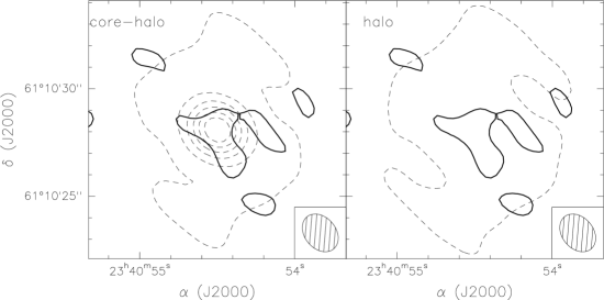
Figure 19: Left panel: map of the C¹⁷O (1–0) line in the peak channel (at $-50.5$ km s^-1 ). The solid contour represents the observed 2$\sigma$ level ($\sim 0.024$ Jy beam^-1), while the dashed contours indicate the emission of a “core-halo” source model, as described in Fig. 17. Levels range from $0.024$ to 0.14 by 0.024 Jy beam^-1. Right panel: same as left for a source model without the central core. Both contours represent the $2\sigma$ observed level.

5.3 The nature of I23385

Here we want to find out whether our results may be used to establish the nature and the evolutionary stage of the embedded YSO.

In cores where the gas is heated by an embedded star, the gas temperature at a radial distance $R=\theta d$ from the central star is expected to scale as (see e.g. Plume et al. plume (1997)):

$$T\propto\left(\frac{L^{1/2}}{\theta d}\right)^{\alpha}$$ (3)

where $L$ is the luminosity of the embedded star. Eq. (3) represents the gas temperature, but at densities as high as $10^{6}$ cm^-3 we can assume coupling between gas and dust. Hence, at such densities Eq. (3) also describes the dust temperature. The index $\alpha$ depends on the opacity index, $\beta$, (Doty & Leung doty (1994)), and it lies between 0.3 and 0.5. The steepest power law is obtained when $\alpha=0.5$, and it corresponds to the optically thick case, when the luminosity irradiated at the core surface $R$ equals the stellar luminosity, namely:

$$L_{*}=4\pi R^{2}\sigma T^{4}\;,$$ (4)

where $T$ represents the surface temperature. If instead the core is optically thin, the temperature profile is flatter. Therefore, the core temperature predicted by Eq. (4) represents a “lower limit”, and at 0.017 pc (corresponding to the radius of I23385 deduced from the CH₃C₂H PdBI emission) for a central star with luminosity $L\sim 1.6\;10^{4}L_{\odot}$ this lower limit is $\sim 51$ K. The temperature derived from CH₃C₂H is significantly lower than that. This discrepancy is confirmed by theoretical models: Osorio & Lizano (osorio (1999)) have performed a theoretical simulation of the temperature profile of I23385 assuming a source luminosity of $\sim 10^{4}L_{\odot}$, deriving a temperature much higher than 42 K at the same radius (see their Fig. 5). To compare our result with what found in HCs, in Fig. 20 we plot the temperature $T$ at the core surface versus $L^{1/2}/R$, for a sample of HCs and for I23385. The luminosity $L$ of the central star is given by the IRAS luminosity for HCs without an embedded Hii regions, and it represents an upper limit. For those with an embedded Hii region, the luminosity of the central star has been deduced from the radio continuum flux of the embedded Hii region (Wood & Churchwell w&c (1989)).

The drawn line indicates the steepest power law, $T\propto(L^{1/2}/R)^{0.5}$. It is evident that it is not possible to match our temperature estimate with that expected for such a power law. To solve this problem we examine three possibilities:

1) We might be overestimating the source luminosity. In Sect. 4.1 we discussed that the luminosity of the embedded source is of the order of $10^{4}$ solar luminosities. This was based on the hypothesis that the bulk of the IRAS fluxes at 60 and 100 $\mu$m is due to I23385. Unfortunately, the IRAS angular resolution is not sufficient to confirm this hypothesis. Hence, the “bright ring” surrounding I23385 might emit a consistent fraction of the flux at 60 and 100 $\mu$m. In that case, the luminosity of I23385 might be lower. A temperature of 42 K at 0.017 pc in an optically thick core implies a central source of $\sim 1.5\;10^{3}L_{\odot}$. Altough well below the value predicted in Sect. 3.3.2, this luminosity is consistent with an intermediate-mass protostar deriving its luminosity from accretion, as shown by Behrend & Maeder (behrend (2001)). In fact, the authors performed calculations of the evolution of protostars with mass from 1 to 85 $M_{\odot}$, assuming growing accretion rates. For an accretion luminosity of $\sim 1.5\;10^{3}L_{\odot}$, the protostar mass is $\sim 6\;M_{\odot}$.

2) Another possibility is that we have underestimated the core diameter. This is possible if the source is not gaussian: in fact, if the core is spherical, the diameter estimated in Table 5 requires a correction (see Panagia & Walmsley pana (1978)). In our case one obtains $\sim 2$^′′(0.047 pc), for the diameter of the core. This brings the luminosity to $3\;10^{3}{\rm L_{\odot}}$, still much less than the value obtained in Sect. 4.1 from the continuum spectrum.

3) Finally, it is possible that the temperature profile, is steeper in case of a non-spherical geometry, as in the presence of a disk. Cesaroni et al. (cesa98 (1998)) have found that HCs are likely to be disk-like structures, in which the temperature profile is $T\propto R^{-0.75}$. With this power-law it is possible to obtain a lower temperature at 0.017 pc with a luminosity of 1.6 $10^{4}{\rm L_{\odot}}$.

Which solution is correct? Concerning the second hypothesis (underestimate of the core radius), we have already seen that it is very unlikely. This is also valid for the third one (disk-like structures): in fact, to measure such a low temperature, the disk should lie along the line of sight, but unfortunately this is more likely “face-on”, because the outflow detected by Molinari et al. (1998b ) lie approximately along the line of sight. The first hypothesis (overestimate of the core luminosity) is the most likely, but presently it is impossible to give a reliable answer, because the correct source luminosity can be derived only by means of a map at $\sim$ 100 $\mu$m at high angular resolution, which is not available. However, as already discussed, a luminosity as low as $10^{3}$ $L_{\odot}$ is consistent with a protostar in the accretion phase, whose mass, at present, is $\sim 6\;M_{\odot}$.

Figure 20: Kinetic temperature measured at the surface of molecular cores plotted against the distance-independent ratio $L^{1/2}/\theta$, where $\theta$ is the angular diameter of the core, and $L$ the luminosity of the embedded (proto)star. Open circles indicate HCs (Kurtz et al. kurtz (2000)) while the filled circle corresponds to I23385. The straight line represents the steepest power law for spherical cores, $T\propto(L^{1/2}/\theta d)^{0.5}$, expected for a dusty core heated by an embedded star (Doty & Leung doty (1994)).

6 Conclusions

We have used the IRAM-30m telescope, the Plateau de Bure Interferometer and the Very Large Array to observe the massive protostar candidate IRAS 23385+6053 in the C¹⁸O (1–0), C¹⁷O (1–0) and (2–1), CH₃C₂H (6–5), (8–7) and (13–12), NH₃ (1,1) and (2,2) lines. The following results have been obtained:

• The source consists of two regions: a compact molecular core with a diameter $\sim 0.03\div 0.04$ pc and a halo which has a diameter of up to $\sim 0.4$ pc; the core has a kinetic temperature of $T_{\rm k}\sim 42$ K and a $\rm H_{2}$ volume density of the order of $n_{\rm H_{2}}\sim 10^{7}$ cm^-3; the halo has an average temperature $T_{\rm k}\sim 15$ K and an average $\rm H_{2}$ volume density $n_{\rm H_{2}}\sim 3\;10^{5}$ cm^-3;

• based on the continuum spectrum, the source luminosity can vary between $1.6\;10^{4}$ and $1.5\;10^{2}\;L_{\odot}$: we believe that the upper limit is closer to the real source luminosity;

• by comparing the $\rm H_{2}$ volume density derived at different radii from the IRAS source, we deduce that the halo has a density profile of the type $n_{\rm H_{2}}\propto r^{-2.3}$, suggesting that it might be gravitationally unstable. This is further supported by the fact that, assuming a density profile as above, the virial mass is much lower than the gas mass.

• On the basis of the steepest theoretical temperature profile expected in cores heated by embedded stars ($T\propto R^{-0.5}$), it is impossible to explain a temperature of 42 K at the core radius, if the source luminosity is $L\sim 10^{4}{\rm L_{\odot}}$. We propose three possible solutions: 1) we are overestimating the stellar luminosity. A temperature of $42$ K at the core radius ($\sim 0.017$ pc) is possible if the stellar luminosity is $\sim 10^{3}{\rm L_{\odot}}$. This solution is consistent with an intermediate-mass protostar deriving its luminosity from accretion; 2) we are underestimating the core radius in case of non-gaussian source, but this solution is unlikely because the correction that we should apply is very small; 3) the source is not spherical: in that case the temperature profile is expected to be steeper ($T\propto R^{-0.75}$) and it is possible to reach a temperature as low as 42 K at the core radius even with luminosities as high as $10^{4}{\rm L_{\odot}}$.

  The first hypothesis seems the most likely, although the real source luminosity can be derived only with high resolution maps at FIR wavelengths, which will become feasible only with the HERSCHEL satellite.

- (1) Bergin, A.E., Goldsmith, P.F., Snell, R.L., Ungerechts, H. 1994, ApJ, 431, 674
- (2) Behrend, R. & Maeder, A. 2001, A&A, 373, 190
- (3) Beuther, H., Schilke, P., Sridharan, T.K., Menten, K.M., Walmsley, C.M., Wyrowski, F. 2002a, A&A, 383, 892
- (4) Beuther, H., Walsh, A., Schilke, P., Sridharan, T.K., Menten, K.M.; Wyrowski, F. 2002b, A&A, 390, 289
- (5) Brand, J., Cesaroni, R., Palla, F., Molinari, S. 2001, A&A, 370, 230
- (6) Cesaroni R., Olmi L., Walmsley C.M., Churchwell E., Hofner P. 1994, ApJL, 435, L137
- (7) Cesaroni R., Hofner P., Walmsley C.M., Churchwell E. 1998, A&A, 331, 709
- (8) Codella C., Testi L., Cesaroni R. 1997, A&A, 325, 282
- (9) Doty, S.D., Leung C.M. 1994, ApJ, 424, 729
- (10) Fontani, F., Cesaroni, R., Caselli, P., Olmi, L. 2002, A&A, 276, 489
- (11) Holland, W.S., Cunningham, C.R., Gear, W.K., Jenness, T., Laidlaw, K. et al. 1998, SPIE, 3357, 305
- (12) Kurtz, S., Cesaroni, R., Churchwell, E., Hofner, P., Walmsley, C. M. 2000, Protostars and Planets IV, 299
- (13) Kutner, M.L. & Ulich, B.L. 1981, ApJ, 250, 341
- (14) MacLaren, I., Richardson, K.M., Wolfendale, A.W. 1988, ApJ, 333, 821
- (15) Molinari S., Brand J., Cesaroni R., Palla F. 1996, A&A, 308, 573
- (16) Molinari S., Brand J., Cesaroni R., Palla F., Palumbo G.G.C. 1998a, A&A, 336, 339
- (17) Molinari, S., Testi, L., Brand, J., Cesaroni, R., Palla, F. 1998b, ApJ 505, L39
- (18) Molinari, S., Brand, J., Cesaroni, R., Palla, F. 2000, A&A, 355, 617
- (19) Molinari, S., Testi, L., Rodriguez, L.F., Zhang, Q. 2002, ApJ, 570, 758
- (20) Myers P.C., Ladd E.F. 1993, ApJ, 413, L47
- (21) Olmi L., Cesaroni R., Neri R., Walmsley C.M. 1996, A&A, 315, 565
- (22) Osorio, M. & Lizano, S. 1999, ApJ, 525, 808
- (23) Palla F., Brand J., Cesaroni R., Comoretto G., Felli M. 1991, A&A, 246, 249
- (24) Panagia, N., Walmsley, C.M. 1978, A&A, 70, 411
- (25) Penzias, A.A. 1981, ApJ, 249, 518
- (26) Plume, R., Jaffe, D.T., Evans II, N.J., et al. 1997, ApJ, 476, 730
- (27) Preibisch, Th., Ossenkopf, V., Yorke, H.W., Henning, Th. 1993, A&A, 279, 577
- (28) Ruffle, D.P., Hartquist, T.W., Taylor, S.D., Williams, D.A. 1997, MNRAS, 291, 235R
- (29) Shu, F.H., Adams, F.C., Lizano, S. 1987, ARA&A, 25, 23
- (30) Spitzer, L. 1978, Physical processes in the intestellar medium (John Wiley & Sons, Inc.)
- (31) Testi L., Natta A., Shepherd D.S., Wilner D.J. 2003, A&A 403, 323
- (32) Thompson, M.A. & Macdonald, G.H. 2003, A&A, in press
- (33) Townes, C.H. & Schawlow, A.L. 1975, Microwave spectroscopy (Dover, New York)
- (34) Ungerechts, H., Walmsley, C.M., Winnewisser, G. 1986, A&A, 157, 207
- (35) Van Dishoeck, E.F., Blake, G.A. 1998, ARA&A, 36, 317
- (36) Wang, T.Y.,Wouterloot, J.G.A., Wilson, T.L. 1993, A&A, 277, 205
- (37) Wilner, D.J., Welch, W.J. 1994, ApJ 427, 898
- (38) Wilner D.J., Ho P.T.P., Kastner J.H., Rodriguez L.F. 2000, ApJ 534, L101
- (39) Wilson, T.L., & Rood, R.T. 1994, ARA&A, 32, 191
- (40) Wood, D.O.S., & Churchwell, E. 1989, ApJ, 340, 265
- (41) Wyrowski, F. 1997, Ph.D. thesis, Univ. of Cologne