Amount of intergalactic dust: constraints from distant supernovae and thermal history of intergalactic medium

Abstract

This paper examines the allowed amount of IG (intergalactic) dust, which is constrained by extinction and reddening of distant SNe Ia and thermal history of IGM (intergalactic medium) affected by dust photoelectric heating. Based on the observational cosmic star formation history, we find an upper bound of $\chi$, the mass ratio of the IG dust to the total metal in the Universe, as $\chi\la 0.1$ for $10{\rm\AA}\la a\la 0.1\micron$ and $\chi\la 0.1(a/0.1\,\micron)$ for $0.1\micron\la a\la 1\micron$, where $a$ is a characteristic grain size of the IG dust. This upper bound of $\chi\sim 0.1$ suggests that the dust-to-metal ratio in the IGM is smaller than the current Galactic value. The corresponding allowed density of the IG dust increases from $\sim 10^{-34}$ g cm^-3 at $z=0$ to $\sim 10^{-33}$ g cm^-3 at $z\sim 1$, and keeps almost the value toward higher redshift. This causes IG extinction of $\la 0.2$ mag at the observer’s $B$-band for $z\sim 1$ sources and that of $\la 1$ mag for higher redshift sources. Furthermore, if $E(B-V)\sim 0.1$ mag at the observer’s frame against $z\ga 1$ sources is detected, we can conclude that a typical size of the IG dust is $\la 100$ Å. The signature of the 2175 Å feature of small graphite may be found as a local minimum at $z\sim 2.5$ in a plot of the observed $E(B-V)$ as a function of the source redshift. Finally, the IGM mean temperature at $z\la 1$ can be still higher than $10^{4}$ K, provided the size of the IG dust is $\la 100$ Å.

1 Introduction

As long as there is dust between radiation sources and observers, the dust extinction and reddening must be corrected if we want to realize the nature of the sources. We should examine how much extinction and reddening there are. The extinction property in the Galaxy is a well studied example (e.g., Draine & Lee 1984). Using HI and far-infrared emission as tracers for the dust column density, we can obtain the extinction amount by the Galactic dust with reasonable accuracy (Burstein & Heiles, 1982; Schlegel, Finkbeiner, & Davis, 1998). Although the dust distribution and properties in the external galaxies are not well known yet, we can correct the dust extinction in the galaxies by using some indicators of the extinction with some assumptions (e.g., Buat et al. 2002). How about the extinction by the intergalactic (IG) dust?

We have already known the fact that some metal elements exist in the Lyman $\alpha$ clouds even at redshift larger than 3 (e.g., Cowie et al. 1995; Telfer et al. 2002). It suggests that the dust grains also exist in the low-density intergalactic medium (IGM). Such diffuse IG dust causes the IG extinction and reddening, which may affect on our understanding of the Universe significantly. One might think that the IG dust amount is negligible because such a significant IG reddening is not reported in the previous studies (Takase, 1972; Cheng, Gaskell, & Koratkar, 1991; Riess et al., 1998; Perlmutter et al., 1999). However, the wavelength dependence of the IG extinction is quite uncertain. If it is gray as suggested by Aguirre (1999), a large extinction is possible with no reddening. Nobody can conclude that the IG dust is negligible because of no observable reddening.

Theoretically, it is predicted that metals synthesized in supernova (SN) explosions form into the dust grains in the cooling ejecta of SNe (Kozasa & Hasegawa, 1987; Todini & Ferrara, 2001; Nozawa et al., 2003; Schneider, Ferrara, & Salvaterra, 2003). Recently, thermal emissions of such dust from two supernova remnants, Cas A and Kepler, are detected (Dunne et al., 2003; Morgan et al., 2003). In a very high-$z$ universe, SNe of massive Population III stars formed in low mass halos, which are likely to be the main site of the first star formation, can disperse the produced metals into the IGM (Bromm, Yoshida, & Hernquist, 2003). The dust grains may be also dispersed into the IGM. Therefore, the IG dust grains may exist even in a $z\ga 10$ universe (Elfgren & Désert, 2003).

Extinction by the IG dust may affect on the determination of the cosmological parameters from observations of SNe. The observed dimming beyond the geometrical dimming in the empty space of distant ($z\simeq 0.5$) Type Ia SNe, which is attributed to the cosmological constant (Riess et al., 1998; Perlmutter et al., 1999), can be reproduced by the gray IG extinction without the cosmological constant (Aguirre, 1999). Goobar, Bergstöm, & Mörtsell (2002) show that the apparent brightening of the farthest SNe Ia ($z=1.7$; Riess et al. 2001) can be also explained by the gray IG extinction with zero cosmological constant if the dust-to-gas ratio in the IGM decreases properly with increasing redshift. Therefore, to know the amount of the IG dust is also important in the cosmological context.

The evidence of the IG dust should be imprinted in the cosmic microwave background (CMB) and infrared background because the dust emits thermal radiation in the wave-band from the far-infrared to submillimetre (submm) (Rowan-Robinson, Negroponte, & Silk, 1979; Wright, 1981; Elfgren & Désert, 2003). Although the COBE data provides us with only a rough upper bound on the IG dust (Loeb & Haiman, 1997; Ferrara et al., 1999; Aguirre & Haiman, 2000), the data of WMAP (Spergel et al., 2003) may be promising. The submm background radiation will give a more strict constraint on the IG dust (Aguirre & Haiman, 2000).

Recently, we have proposed a new constraint on the IG dust amount by using thermal history of the IGM (Inoue & Kamaya, 2003). Since the dust photoelectric heating is very efficient in the IGM (Nath, Sethi, & Shchekinov, 1999), the theoretical thermal evolution of the IGM taking into account of the heating by dust violates the observational temperature evolution if too much IG dust is input in the model. Hence, Inoue & Kamaya (2003) obtain an upper bound of the IG dust amount in order that the theoretical IGM temperature should be consistent with the observed one. The obtained upper bound of the dust-to-gas ratio in the IGM is 1% and 0.1% of the Galactic one depending on the IG grain size of $\sim 100$ Å– 0.1 $\mu$m and $\sim 10$ Å, respectively, at redshift of $\sim 3$.

In this paper, with help of distant SNe Ia observation, we extend our previous approach in order to discuss the upper bounds of the IG dust extinction and reddening. In the next section, we start from the cosmic star formation history (SFH) to specify the IG dust amount at each redshift. According to the assumed SFH, we can estimate IG dust extinction and reddening at each redshift theoretically. In section 3, we comment on observational constraints from the extinction and reddening of distant SNe Ia. In section 4, further constraints are presented by comparing theoretical and observational thermal histories of the IGM. Based on the allowed amount of the IG dust, we also discuss some implications from our results in section 5. The achieved conclusions are summarised in the final section.

Throughout the paper, we stand on a $\Lambda$-cosmology. That is, we constrain the amount of the IG dust in order that the IG dust should not affect on the determination of the cosmological parameters from distant SNe Ia. This is because the flat universe is favored by results of CMB observations (Jaffe et al., 2001; Pryke et al., 2002; Spergel et al., 2003), whereas only the matter cannot make the flat universe (Percival et al., 2001). Furthermore, the recent observations of the X-ray scattering halo around high-$z$ QSOs suggest too small amount of the IG dust to explain all amount of the dimming of the distant SNe Ia (Paerels et al., 2002; Telis et al., 2002, but see also Windt 2002). Mörtsell & Goobar (2003) also reach the same conclusion by analyzing the observed colours of the SDSS (Sloan Digital Sky Survey) quasars. The following cosmological parameters are adopted: $H_{0}=70$ km s^-1 Mpc^-1, $\Omega_{\rm M}=0.3$, $\Omega_{\Lambda}=0.7$, and $\Omega_{\rm b}=0.04$.

2 Star formation history and intergalactic dust

To estimate the IG extinction and reddening theoretically, we must investigate production of dust at each redshift. Since dust is made of metals, a cosmological evolution of the metal amount should be specified. As metals are products of stellar evolution, therefore, we shall specify the cosmic SFH as a first step.

Since Madau et al. (1996), researches of the cosmic SFH are extensively performed. In figure 1, we show observational star formation rates in a unit comoving density as a function of redshift. The cross and open symbols are estimated from the H$\alpha$ line and the rest-frame ultra-violet (UV) luminosities not corrected by the interstellar dust extinction. Hence these are lower limits. The filled-circles are estimated from the submm data. Due to the small statistics, the uncertainty of the submm data is rather large. The real SFH is still uncertain because we do not know the suitable correction factor against the internal dust extinction. In this paper, therefore, we adopt two example models: high and low SFHs, which are shown in figure 1 as solid and dashed curves, respectively. For the low SFH case, we have employed a conservative correction factor for the internal dust extinction. The high SFH case is set to be compatible with the submm data. Quantitatively, these SFHs are formulated as

$$\frac{\rho_{\rm SFR}^{*}(z)}{0.1M_{\odot}\,{\rm yr}^{-1}\,{\rm Mpc}^{-3}}=\cases{\left(\frac{1+z}{2}\right)^{3.3}&(for $z\leq 1$)\cr\left(\frac{1+z}{2}\right)^{-1.5}&(for $z>1$ low SFH)\cr 1&(for $z>1$ high SFH)\cr}\,,$$ (1)

where $\rho_{\rm SFR}^{*}$ is the star formation rate per unit comoving density. Recently, some authors suggest that a SFH like the high case is more likely (e.g., Springel & Hernquist, 2003; Giavalisco et al., 2004). Hence, we discuss the high SFH case mainly in the following.

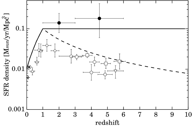
Figure 1: Cosmic star formation rate density as a function of redshift. The plotted points with error-bars are estimated from the H$\alpha$ data: cross (Gallego et al., 1995) and inclined cross (Tresse & Maddox, 1998); from the rest-frame ultra-violet data: open-triangles (Lilly et al., 1996), open-diamonds (Connolly et al., 1997), open-pentagons (Madau, Pozzetti, & Dickinson, 1998), open-circles (Steidel et al., 1999), open-squares (Giavalisco et al., 2004), open-inverse-pentagon (Iwata et al., 2003), open-inverse-triangle (Bouwens et al., 2003); and from the submillimetre data: filled-circles (Barger, Cowie, & Richards, 2000). These points are adjusted to the cosmological parameters assumed in this paper. The solid and dashed curves are the models of high and low star formation histories, respectively.

Once a SFH is specified and if the instantaneous recycling approximation is adopted, the cosmic mean metallicity evolution is determined by:

$$Z(z)=\frac{y_{Z}}{\Omega_{\rm b}\rho_{\rm c,0}}\int_{z}^{z_{\rm S}}\rho_{\rm SFR}^{*}(z^{\prime})\frac{dz^{\prime}}{H(z^{\prime})(1+z^{\prime})}\,,$$ (2)

where $y_{Z}$ is the produced metal mass fraction for a unit star forming mass, $\rho_{\rm c,0}$ is the current critical density, $z_{\rm S}$ is the starting redshift of the cosmic star formation, and $H(z)$ is the Hubble constant at the redshift $z$. We have assumed $y_{Z}$ to be a constant for simplicity. If the Salpeter initial mass function (0.1–125 $M_{\odot}$) is assumed, $y_{Z}=0.024$ (Madau et al., 1996). We assume $z_{\rm S}=10$ in this paper. This does not affect on the results obtained in the following sections because the measure of time along the redshift is small in the high-$z$ universe. Indeed, the cosmic metallicities in $z\la 3$ for various $z_{\rm S}$ become nearly equal to each other if $z_{\rm S}\ga 5$.

In figure 2, we show the mean cosmic metallicity as a function of redshift. In the figure, the lower limit of metallicity in the Ly$\alpha$ clouds measured from C IV and Si IV by Songaila (2001) and the ranges of carbon abundance obtained by Schaye et al. (2003) and oxygen abundance obtained by Telfer et al. (2002) are overlaid. Our theoretical estimate of total metallicity in the universe is compatible with the observed oxygen abundance in the IGM. This may mean that a large part ($\sim 50$%) of metal produced in galaxies exist out of galaxies. On the other hand, our estimate is much larger than the observed carbon abundance. This may indicate that carbon is not suitable to trace the cosmic mean metallicity in the early phase since the first metal pollution is made by the Type II SNe (e.g., Pagel, 1997). Indeed, Aguirre et al. (2004) find [Si/C]$\sim 0.8$.

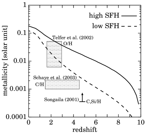
Figure 2: Mean cosmic metallicity evolution. The vertical axis is normalized by the Solar metallicity $Z_{\odot}=0.02$. The solid and dashed curves are the cases of the high and low star formation histories, respectively. The starting redshift of the cosmic star formation is set to be $z_{\rm S}=10$. The observed range of oxygen abundance by Telfer et al. (2002), carbon abundance by Schaye et al. (2003), and lower limit of metallicity obtained by Songaila (2001) are overlaid as the shaded squares and the upward arrow, respectively. We note that Aguirre et al. (2004) find [Si/C]$\sim 0.8$.

Let us introduce one parameter to describe the amount of the IG dust; the ratio of the IG dust mass to the total metal mass in the universe defined as

$$\chi\equiv\frac{\rm IG\,dust\,mass}{\rm total\,metal\,mass}=\frac{{\cal D}^{\rm IGM}}{Z}\,,$$ (3)

where ${\cal D}^{\rm IGM}$ is the dust-to-gas mass ratio in the IGM. In principle, this parameter is determined by the transfer mechanism of dust grains from galaxies into the IGM. Although some authors have tried to solve this problem approximately (e.g., Ferrara et al. 1990, 1991; Aguirre et al. 2001), the results are not still conclusive. This is because we must solve problems of the magneto-radiation-hydrodynamics of dusty plasma finally. Here we approach the parameter $\chi$ by another way; we constrain the parameter by using the observational data of distant SNe Ia (§3) and the thermal history of the IGM (§4). While the parameter $\chi$ may evolve along redshift, we treat it as a constant for simplicity. Hence, the obtained values of $\chi$ in the following sections are regarded as those averaged over redshift.

A dust model must also be specified. In this paper, we adopt the “graphite” and the “smoothed astronomical silicate” models by Draine & Lee (1984); Laor & Draine (1993); Weingartner & Draine (2001a), which can explain the interstellar dust properties in the Galaxy and the Magellanic clouds very well. Although there is no evidence that the IG dust is the same as the Galactic dust, we assume them as a working hypothesis.

The grain size distribution in the IGM is also quite uncertain. As a first step, we assume all grains to have the same size. This means that the grain size in the current paper indicates a characteristic size of the IG dust (i.e. an averaged size by a certain way). Aguirre (1999) suggests a selection rule in the transfer of dust grains from the host galaxies into the IGM; the small grains are destroyed by the thermal sputtering process when the grains are transfered through the hot gas halo of the host galaxies. Indeed, this theoretical suggestion is very interesting to realize the gray dust model. However, we also examine the possibility of the small IG grain because the suggestion of the selection rule is not confirmed observationally at the moment.

3 Constraint from observational dimming of supernovae

In this section, we constrain the amount of the IG dust by means of observational dimming of distant Type Ia SNe. According to Riess et al. (2001), the dimming of SNe Ia at $z\sim 0.5$ is $\sim 0.2\pm 0.1$ mag against the empty universe. Our policy is that the IG dust extinction does not affect the interpretation of the cosmological constant. Thus, we attribute the 0.2 mag dimming of SNe Ia at $z\sim 0.5$ to the cosmological constant and regard the quoted error (0.1 mag) as an upper limit of the contribution by the IG dust to the dimming. Although the cosmological dimming does not depend on the observed wavelength, the dimming by the IG dust may depend on the wavelength. As the distant SNe Ia are observed in $B$ and $V$-bands and $B$-band provides a slightly more strict constraint of the IG dust than $V$-band, we regard the upper limit of 0.1 mag as that in the $B$-band. In addition, Perlmutter et al. (1999) report that the difference of the observed reddening between the local and distant SNe is $\langle E(B-V)\rangle_{z=0.5}-\langle E(B-V)\rangle_{z=0.05}=0.002\pm 0.03$ mag. Although there seems to be no systematic difference, we can still consider the absolute value of the colour excess by the IG dust less than 0.03 mag. In summary, the IG extinction and reddening from observations of distant SNe Ia at $z\sim 0.5$ are $A^{\rm IGM}_{B,z=0.5}\leq 0.1$ mag and $|E(B-V)^{\rm IGM}_{z=0.5}|\leq 0.03$ mag.

Suppose an observer who observes a source with a redshift of $z$ at a wavelength of $\lambda_{\rm obs}$ in his/her rest frame. The amount of the IG extinction is given by

$$\frac{A_{\lambda_{\rm obs}}^{\rm IGM}(z)}{\rm mag}=1.086\pi a^{2}\int_{0}^{z}Q\left(a,\frac{\lambda_{\rm obs}}{1+z^{\prime}}\right)n_{\rm d}^{\rm IGM}(z^{\prime})\frac{c\,dz^{\prime}}{(1+z^{\prime})H(z^{\prime})}\,,$$ (4)

where $a$ is the grain radius, $Q$ is the extinction efficiency factor, $c$ is the light speed, and $n_{\rm d}^{\rm IGM}$ is the IG grain number density in a unit physical volume, which is

$$n_{\rm d}^{\rm IGM}(z)=\frac{\chi\Omega_{\rm b}\rho_{\rm c,0}(1+z)^{3}Z(z)}{4\pi a^{3}\varrho/3}\,,$$ (5)

where $\varrho(=2\,{\rm g\,cm^{-3}})$ is the grain material density. For simplicity, we have assumed that dust grains distribute uniformly with $n_{\rm d}^{\rm IGM}$ corresponding to the redshift. We do not consider any structure of the dust distribution.

In figure 3, we show the amount of the IG extinction divided by $\chi$ for a source with $z=0.5$ as a function of the assumed grain size. While the results for the high SFH is depicted in the figure, the extinction amount for the low SFH case is only a factor of about 1.5 smaller than that of the high SFH case. The extinction amount is independent of the grain size as long as $2\pi a<\lambda$. This is caused by (1) the extinction cross section ($=Q_{\rm ext}\pi a^{2}$) is proportional to $a^{3}$ because the extinction efficiency factor, $Q_{\rm ext}$, is proportional to the grain size, $a$, linearly, and (2) the number density of the grain has a dependence of $a^{-3}$ for a fixed dust mass. On the other hand, $Q_{\rm ext}$ becomes constant (almost 2) when $2\pi a>\lambda$, so that the extinction cross section is determined by mainly the geometrical one which is proportional to $a^{2}$. Thus, the extinction amount is proportional to $a^{-1}$. When $2\pi a\sim\lambda$, grains interact with photons the most effectively, so that the amount of extinction shows a peak in both panels of figure 3.

Figure 3: Intergalactic extinction in various bands against a source with the redshift $z=0.5$ as a function of the IG grain size. The vertical axis is divided by the parameter $\chi$, which is defined by equation (3). The panels (a) and (b) are the cases of silicate and graphite, respectively. The star formation history assumed is the lower case shown in figure 1. The solid curves indicate the extinction amount in the $U$, $B$, $V$, $R$, $I$, $J$, $H$, and $K$ bands from top to bottom.

We shall remember the observational constraints of $A_{B,z=0.5}^{\rm IGM}\leq 0.1$ mag and $|E(B-V)^{\rm IGM}_{z=0.5}|\leq 0.03$ mag. Hence, we can obtain the upper bound of $\chi$ via Eq.(4) or figure 3, which is shown in figure 4. The silicate and graphite cases are shown in the panel (a) and (b), respectively. The dotted and dashed curves indicate the upper bounds of $\chi$ based on $A_{B,z=0.5}^{\rm IGM}=0.1$ mag and $|E(B-V)^{\rm IGM}_{z=0.5}|=0.03$ mag, respectively. The discontinuity of the dashed curve is due to $E(B-V)=0$; the left of the discontinuity is positive $E(B-V)$ and the right is negative one. The solid curve is the upper bound based on the thermal history of the IGM which is obtained in the next section. The rejected area of $\chi$ is shaded; the thin shade means the rejected area based on the SNe Ia extinction/reddening, and the thick shade is the area based on the IGM thermal history (section 4). We show only the high SFH case.

We find that, for both grain types, the upper bound of $\chi$ from the distant SNe Ia is $\sim\ 0.1(a/0.1\,{\rm\mu m})$ for $0.1\,{\rm\mu m}\la a\la 1\,{\rm\mu m}$. While we have no constraint of $\chi$ for the small ($a\la 100$ Å) silicate grain (panel [a]), the upper bound of $\chi$ is $\sim 0.1$ when $a\la 100$ Å for the graphite case (panel [b]). This difference is caused by the different optical properties between graphite and silicate; small silicate is more transparent than graphite in the optical bands. For $100\,{\rm\AA}\la a\la 0.1\,{\rm\mu m}$, the upper bound of $\chi$ shows a local minimum corresponding to the peak shown in figure 3. Finally, there is not any constraint of $\chi$ for a very large ($a\ga 1$ $\mu$m) grain.

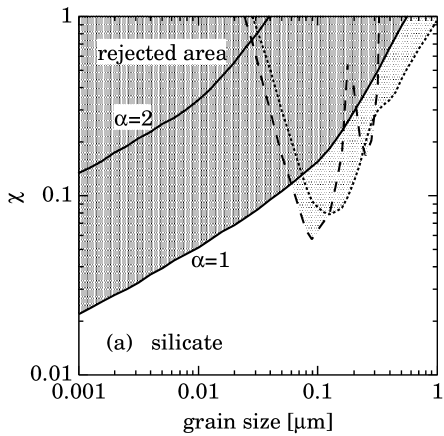
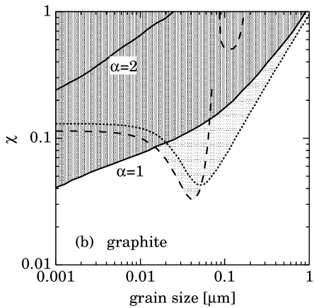
Figure 4: Rejected area of $\chi$, the mass ratio of the IG dust to the total metal as a function of the IG grain size: (a) silicate and (b) graphite case. The dotted and dashed curves are the upper bounds from extinction and reddening of distant SNe Ia. The solid curves are the upper bound obtained from the thermal history. Two spectral indices of the background radiation are considered; $\alpha=1$ (bottom solid) and 2 (top solid). The thick and thin shaded areas are the rejected areas based on the thermal history ($\alpha=1$ case) and on observations of SNe Ia, respectively. The high SFH is assumed.

4 Constraint from IGM thermal history

As shown in the previous paper (Inoue & Kamaya 2003), we show that the amount of the IG dust is constrained by using the thermal history of the IGM. When a dust grain is hit by a photon with an energy larger than a critical value, an electron escapes from the grain; photoelectric effect. Such a photoelectron contributes to the gas heating if its energy is larger than the mean kinetic energy of gas particles. As shown in Appendix A (see also Nath, Sethi, & Shchekinov 1999; Inoue & Kamaya 2003), the photoelectric heating by dust grains is comparable with, and sometimes dominate, the atomic photoionization heating in the IGM. Of course, the efficiency of the dust heating depends on the dust amount. If a model of the IGM has too much dust, the theoretical temperature of IGM exceeds the observational one owing to the dust photoelectric heating. Therefore, we can put an upper bound of the amount of the IG dust so as to keep the consistency between the theoretical IGM temperature and the observed one. In the next subsection, we describe how to calculate the thermal history of IGM affected by the dust photoelectric heating. An upper bound of $\chi$, which represents the amount of the IG dust, is estimated in subsection 4.2.

4.1 Thermal history of IGM

In this paper, we consider only a mean temperature of the IGM, $T_{\rm IGM}$, for simplicity. The $T_{\rm IGM}$ time-evolution is described by (e.g., Hui & Gnedin 1997)

$$\frac{dT_{\rm IGM}}{dt}=-2HT_{\rm IGM}-\frac{T_{\rm IGM}}{X}\frac{dX}{dt}+\frac{2(\Gamma-\Lambda)}{3k_{\rm B}Xn_{\rm b}}\,,$$ (6)

where $H$ is the Hubble constant, $n_{\rm b}$ is the cosmic mean number density of baryon, $\Gamma$ and $\Lambda$ are the total heating and cooling rates per unit volume, respectively, $X$ is the number ratio of the total gaseous particles to the baryon particles, i.e., $X\equiv\sum n_{i}/n_{\rm b}$, where $n_{i}$ is the number density of the $i$-th gaseous species and we consider H i, H ii, He i, He ii, He iii, and electron. We neglect the effect of helium and metal production by stars on the chemical abundance for simplicity. Fortunately, time evolution of their abundance is not important. Indeed, the metal mass fraction reaches at the most $0.002$ (figure 2). The number ratio of helium to hydrogen is always about 0.1 after the Big-bang. A constant mass fraction ($Y=0.24$) of helium is assumed throughout our calculation.

We solve equation (6) coupled with non-equilibrium rate equations for these gaseous species by the fourth-order Runge-Kutta scheme. These rate equations with rate coefficients and the heating/cooling rates are summarised in Appendix B. In the calculation, the time-step is adjusted to being 1/1000 of $-X_{\rm HI}/(dX_{\rm HI}/dt)$ for $dX_{\rm HI}/dt<0$ and $X_{\rm HII}/(dX_{\rm HI}/dt)$ for $dX_{\rm HI}/dt>0$ (see equation [B6] for $dX_{\rm HI}/dt$). The number density of the IG dust at each redshift is determined by equation (1), (2), and (5) depending on $\chi$. The grain charge and heating/cooling rates are determined by a standard manner which is described in Inoue & Kamaya (2003) (see also Appendix A).

The initial condition is as follows: the starting redshift is $z=3.4$, at which it is considered that the HeII reionization occurred (e.g., Theuns et al. 2002a). The initial temperature is set to be 25,000 K, which is the mean IGM temperature at this redshift suggested by the Lyman $\alpha$ forest in QSO spectra (Schaye et al., 2000; Theuns et al., 2002b). We assume an ionization equilibrium balanced between the recombination and the photoionization as the initial chemical abundance. In each time step, the calculated chemical abundance at $z<3.4$ reaches almost another ionization equilibrium balanced among the recombination, the photoionization, and the collisional ionization.

The background radiation is required to calculate the IGM thermal history. We assume a single power-law background radiation; its mean intensity at a frequency of $\nu$ is $J_{\nu}=J_{\rm L}(\nu/\nu_{\rm L})^{-\alpha}$, where $J_{\rm L}$ and $\nu_{\rm L}$ are the mean intensity and the frequency at the hydrogen Lyman limit. We also assume the spectral index $\alpha$ to be constant, but the intensity $J_{\rm L}$ evolves along the redshift. In figure 5, such an evolution is displayed. The data are taken from Scott et al. (2002) who investigate the QSO proximity effect on the number density of the Lyman $\alpha$ forest in spectra of QSOs at $z=0$–5, and estimate the Lyman limit intensity of the background radiation in the redshift range. Here, we use a fitting formula as

$$\frac{J_{\rm L}}{\rm erg\,s^{-1}\,cm^{-2}\,sr^{-1}\,Hz^{-1}}\approx 2.5\times 10^{-23}(1+z)^{2.5}$$ (7)

for $0\la z\la 4$, which is shown in figure 5 as the solid line. The background radiation at $z\la 3$ is likely to be dominated by QSOs. Hence, we consider two cases of $\alpha=1$ and 2. Such values of $\alpha$ are consistent with the QSO dominated background radiation (Haardt & Madau, 1996; Zheng et al., 1997). In appendix A2, we show that the results with $\alpha=1$ single power-law background spectrum should be consistent quantitatively with those with a more realistic spectrum like Haardt & Madau (1996).

Figure 5: Redshift evolution of ionizing background intensity. Data points with error-bars are taken from Scott et al. (2002). The solid line is an analytical fit described in equation (7).

In figure 6, we show some examples of the IGM thermal history, assuming 0.1 µm IG dust and the spectral index of $\alpha=1$. The panel (a) shows the silicate and the high SFH case, and the panel (b) shows the graphite and the low SFH case. In each panel, six cases of $\chi$ are depicted as the solid curves. By definition of $\chi$ (eq.[3]), $\chi=0$ means no IG dust and $\chi=1$ means that all of metal is condensed into the IG dust. The observational data are taken from Schaye et al. (2000). They observe the Ly$\alpha$ clouds with the column density of $10^{13-15}$ cm^-2 (i.e., slightly over density regions), and convert the temperature of the clouds into that at the mean density of the IGM by using the equation of state of the IGM. Thus, we can compare both thermal histories directly. In the next subsection, such a comparison is presented quantitatively.

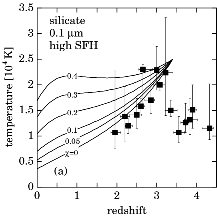
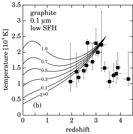
Figure 6: Examples of the IGM thermal history: (a) silicate for high SFH and (b) graphite for low SFH cases. The grain size is assumed to be 0.1 µm. Six solid curves in each panel are the thermal histories assumed a value of $\chi$, the mass ratio of the IG dust to the total metal, indicated on each curve. The data points are taken from Schaye et al. (2000). The spectral index of the background radiation is assumed to be unity.

4.2 Constraint for $\chi$ from thermal history of IGM

Once theoretical histories of IGM temperature are obtained, the amount of IG dust is constrained from the comparison of the theoretical temperature with observational one. Hence, we compare our theoretical thermal histories with 10 observational points at the range of $1.5<z<3.4$ of Schaye et al. (2000). We reject a case of too much $\chi$ by the least squares method. The rejection criterion is the significance level less than 30% in $\chi^{2}$-test. The obtained upper bound of $\chi$ in the high SFH case is shown in figure 4 as the solid curves. In this figure, the results from distant SNe Ia are overlaid as the dotted and dashed curves. Moreover, the rejection areas from the thermal history and distant SNe Ia are distinguished by the thick and thin shadings, respectively.

Combining constraints from the thermal history with those from distant SNe Ia, we obtain the rejected range of $\chi$ as a function of the IG grain size, which are summarised in Table 1. We find a rough upper bound of $\chi$ as 0.1 with a factor of a few uncertainty, except for a very large ($\sim 1$ µm) case and a medium-size ($\sim 100$ Å) silicate of $\alpha=2$.

Table 1: Upper bounds of $\chi$

silicate
$\alpha=1$	low SFH		high SFH
10 Å	0.093	TH	0.022	TH
100 Å	0.22	TH	0.051	TH
0.1 µm	0.096	SNe	0.064	SNe
1 µm	1.0	def	0.97	SNe
$\alpha=2$	low SFH		high SFH
10 Å	0.55	TH	0.13	TH
100 Å	1.0	def	0.34	TH
0.1 µm	0.096	SNe	0.064	SNe
1 µm	1.0	def	0.97	SNe
graphite
$\alpha=1$	low SFH		high SFH
10 Å	0.17	SNe	0.041	TH
100 Å	0.15	SNe	0.076	TH
0.1 µm	0.11	SNe	0.071	SNe
1 µm	1.0	def	0.95	SNe
$\alpha=2$	low SFH		high SFH
10 Å	0.17	SNe	0.11	SNe
100 Å	0.15	SNe	0.10	SNe
0.1 µm	0.11	SNe	0.071	SNe
1 µm	1.0	def	0.95	SNe

The upper bound of $\chi$ from the thermal history has a positive dependence of grain size. This corresponds to the fact that the dust heating rate has a negative dependence of grain size (see figure A3). Especially, for small silicate grain, we obtain a strict upper bound of $\chi$ from the thermal history, whereas observations of distant SNe Ia cannot provide any constraints.

We notice here that the upper bound of $\chi$ for small silicate is smaller than that for small graphite. This is why a small ($a\la 0.1\micron$) silicate has a larger efficiency factor for absorption than that of graphite in the UV–X-ray regime. Hence the grain potential, mean photoelectron energy, and heating rate of small silicate are larger than those of graphite (figures A1–A3). Moreover, we find a positive dependence of the spectral index $\alpha$ against the obtained upper bounds of $\chi$, which is due to the negative dependence of $\alpha$ against the dust heating rate (figure A3).

5 Discussion

We have obtained upper bound of $\chi$ as a function of grain size from observations of distant SNe Ia and comparison of theoretical IGM thermal history with observational one. Here we discuss what our results imply.

5.1 Allowable amount of IG dust

Figure 7: Maximum (a) IG dust density and (b) dust-to-gas mass ratio in the IGM as a function of redshift. In each panel, the solid and dashed curves are the cases of high and low star formation histories, respectively. The assumed $\chi$, the mass ratio of the IG dust to the total metal in the universe, is 0.1.

How much dust can exist in the IGM? Once assuming a value of $\chi$, we obtain the IG dust density via equation (5). In figure 7, we show the upper bounds of the IG dust mass density and ${\cal D}^{\rm IGM}$ as a function of redshift. The solid and dashed curves are the cases of high and low SFHs, respectively. The assumed upper bound of $\chi$ is 0.1 for both cases of SFHs. The uncertainty of this value of $\chi$ is about a factor of a few as long as the IG grain size is smaller than 1 µm and the background spectral index $\alpha=1$ (see also Table 1). We find that the upper bound of the local ($z\sim 0$) universe is determined well; the local IG dust density is less than about $10^{-34}$ g cm^-3, or equivalently the dust-to-gas ratio is less than about $3\times 10^{-4}$ which is about 1/20 of the Galactic value. Along the redshift, the allowed dust density increases and the dust-to-gas ratio decreases. The increasing/decreasing rates change at $z\sim 1$ at which the $(1+z)$ dependence of the assumed SFH changes (eq.[1]). Taking into account a factor of 2 uncertainty of the upper bound of $\chi$, we obtain the maximum IG dust density as

$$\frac{\rho_{\rm d,max}^{\rm IGM}(z)}{\rm g\,cm^{-3}}=(2-8)\times 10^{-34}\cases{\left(\frac{1+z}{2}\right)^{2.3}&(for $z\leq 1$)\cr\left(\frac{1+z}{2}\right)^{0-1.5}&(for $z>1$)\cr}\,,$$ (8)

or the maximum dust-to-gas mass ratio as

$${\cal D}_{\rm max}^{\rm IGM}(z)=(1-4)\times 10^{-4}\cases{\left(\frac{1+z}{2}\right)^{-0.7}&(for $z\leq 1$)\cr\left(\frac{1+z}{2}\right)^{-(1.5-3)}&(for $z>1$)\cr}\,.$$ (9)

The dust-to-gas ratio at $z\sim 3$ is consistent with the previous result by Inoue & Kamaya (2003).

5.2 IG extinction and reddening

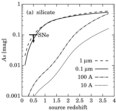
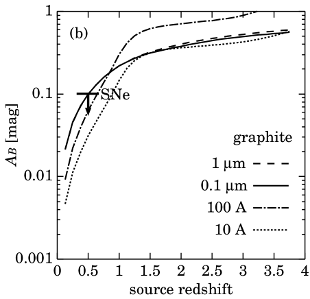
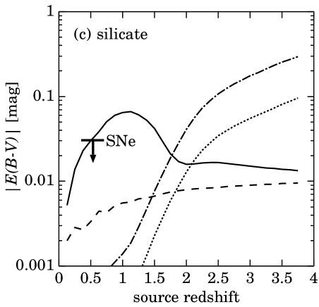
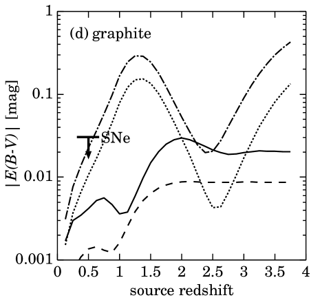
Figure 8: Maximum intergalactic extinction and reddening against a source at a redshift in the case of high star formation history; observer’s $B$-band extinction of (a) silicate case and (b) graphite case, and colour excesses between $B$ and $V$-bands in observer’s rest frame of (c) silicate case and (d) graphite case. Assumed $\chi$ values are summarised in Table 1. For dotted, dot-dashed, solid, and dashed curves, we assumed the grain size of 10 Å, 100 Å, 0.1 µm, and 1 µm, respectively. The spectral index of the background radiation is assumed to be unity. The upper bounds from observations of distant SNe Ia are shown as the downward arrow in each panel. The vertical axes of panels (c) and (d) are the absolute value of the colour excesses. Actually, colour excesses of 1 µm for silicate and of 0.1 and 1 µm for graphite are negative.

In figure 8, we show the upper bounds of IG extinction and reddening expected from the upper bounds of $\chi$ in the case of the high SFH and $\alpha=1$ summarised in Table 1. Four cases of grain size as 10 Å, 100 Å, 0.1 µm, and 1 µm are indicated by dotted, dot-dashed, solid, and dashed curves, respectively. The constraints from SNe Ia observations of $A_{B}\leq 0.1$ mag and $|E(B-V)|\leq 0.03$ mag at $z=0.5$ are also shown as the downward arrow in each panel. We note that the vertical axes of panels (c) and (d) are the absolute value of colour excess. Indeed, colour excesses of 1 µm for silicate, and of 0.1 µm and 1 µm for graphite are negative.

We find that the upper bound of the IG extinction is $\sim 0.2$ mag for a source at $z=1$ from panels (a) and (b) of figure 8. This value agrees well with the result from SDSS quasars data by Mörtsell & Goobar (2003). For $z\ga 1$ objects, the upper bound of the IG extinction becomes $\sim 0.5$ mag, and as an extreme case, we cannot reject the possibility of 1 mag IG extinction for a source at $z\sim 3$.

Interestingly, we can investigate the nature of the IG dust by using the IG reddening. For $z\ga 1$ sources, the expected absolute value of colour excess by the IG grain larger than $\sim 0.1$ µm is very small, at the most $\sim 0.05$ mag, whereas that by a smaller grain can reach 0.1 mag or more. Thus, it may be possible to determine a typical size of the IG grain from observations of colour excess against a source at $z\ga 1$; the detection of $\ga 0.1$ mag colour excess for such a source proves the existence of small ($\la 100$ Å) IG grains. If the IG dust is dominated by such small grains, the composition of the IG dust can be found. The small graphite grains show a prominent absorption feature at 2175 Å. Thus, we expect a local minimum of colour excess for a source at $z\simeq 2.5$ as shown in panel (d) of figure 8. Therefore, if we detect such a change of colour excess along the redshift, we can conclude that many small graphite grains exist in the IGM.

Observations to detect the IG extinction and reddening are very challenging but strongly encouraging. High-$z$ gamma-ray bursts can be good background light sources for such observations (Perna & Aguirre, 2000).

5.3 Ejection efficiency of dust from galaxies

The dust-to-metal mass ratio in the Galaxy, $\delta_{\rm MW}$, is 0.3–0.5 (e.g., Spitzer, 1978; Whittet, 2003). We may consider the dust-to-metal ratio in the IGM, $\delta_{\rm IGM}$ is equal to $\delta_{\rm MW}$, if $\delta_{\rm MW}$ is typical for all galaxies, and metal and dust are ejected together from galaxies to the IGM keeping $\delta_{\rm MW}$. Is this compatible with the obtained upper bound of $\chi\la 0.1$?

A fraction of metal produced by stars in galaxies exists out of galaxies. This metal escape fraction is defined as $f_{\rm Z,esc}$. While $f_{\rm Z,esc}$ is still uncertain, an estimate of it is 50–75% (Aguirre, 1999, and references therein, see also our figure 2). We shall define another parameter of the IGM metallicity; $Z_{\rm IGM}$. Because of $\chi={\cal D}^{\rm IGM}/Z$ and $f_{\rm Z,esc}=Z_{\rm IGM}/Z$, where $Z$ is the total cosmic metallicity, we find $\delta_{\rm IGM}={\cal D}^{\rm IGM}/Z_{\rm IGM}=\chi/f_{\rm Z,esc}$. Unless $f_{\rm Z,esc}$ is less than $\sim 0.5$, $\delta_{\rm IGM}$ is estimated to be smaller than 0.2 if $\chi\la 0.1$. Therefore, our result of $\chi\la 0.1$ with $f_{\rm Z,esc}\sim 0.5$ may indicate that $\delta_{\rm IGM}<\delta_{\rm MW}$.

If that is true, we have to consider some mechanisms to reduce $\delta_{\rm IGM}$ during the dust transfer. For example, dust destruction during the transfer from galaxies to the IGM (Aguirre, 1999), and/or different ejection efficiencies between metal and dust. Time evolution of the dust-to-metal ratio in galaxies may be also important. As shown by Inoue (2003), the dust-to-metal ratio in younger galaxies (i.e., higher-$z$ galaxies) may be much smaller ($\sim 70$% off) than the present value of the Galaxy. In the case, a time-averaged $\delta_{\rm MW}$ can become smaller than the current $\delta_{\rm MW}$ adopted above, so that our constraint of $\chi$ may be cleared. In any case, we cannot obtain a rigid quantitative conclusion at the moment, because uncertainties are still large. Further studies of this issue are very interesting.

5.4 IGM temperature at low redshift

As shown in Nath et al. (1999) and Appendix A, the dust photoelectric heating becomes more efficient for a lower gas density. Although the background intensity decreases along the redshift (figure 5), the decrement of gas density is more efficient than the decrement of the background intensity, so that the importance of the dust heating increases for a lower redshift. While we obtained constraints of the amount of the IG dust from the IGM temperature at $z\simeq 2$–3 in section 4, the IGM temperature at a lower redshift of $z\la 1$ provides us with a further constraint of the IG dust. Therefore, to measure the IGM temperature at $z\la 1$ is very interesting.

Here, we demonstrate how much temperature is allowed by our upper bounds of $\chi$. Figure 9 shows the IGM thermal histories assumed the upper bounds of $\chi$ in Table 1 for the case of background spectral index $\alpha=1$ and high SFH. The dotted, dot-dashed, and solid curves are the case of no IG dust, 100 Å silicate, and 0.1 µm silicate, respectively. We can make a very similar figure for graphite case. The temperatures shown in the figure are upper bounds, which is denoted as $T_{\rm IGM,up}$.

Figure 9: Maximum IGM temperatures corresponding to the upper bounds of $\chi$ in table 1 for the case of silicate, background spectral index of unity, and high SFH. The dotted, dot-dashed, and solid curves are the case of no IG dust, 100 Å, and 0.1 µm, respectively. The data points are taken from Schaye et al. (2000).

After checking all cases listed in table 1, we find that for a smaller ($\la 100$ Å) grain case, except for graphite of $\alpha=2$, $T_{\rm IGM,up}$ at $z\la 1$ is still much higher than 10,000 K. On the other hand, for a larger ($\ga 0.1$ µm) case, except for 1 µm graphite with high SFH and $\alpha=1$, $T_{\rm IGM,up}$ at $z\la 1$ becomes lower than 10,000 K as well as no IG dust case. Therefore, we may conclude that IG grains are small if temperature higher than 10,000 K is observed at $z\la 1$. Conversely, a lower IGM temperature at $z\la 1$ provides us with a very strict constraint against small IG dust.

6 Conclusion

We investigate the amount of the IG dust allowed by current observations of distant SNe Ia and temperature of the IGM. The allowed amount of the IG dust is described as the upper bound of $\chi$, the mass ratio of the IG dust to the total metal mass in the Universe. To specify $\chi$, two models of cosmic history of metal production rate are assumed. That is, we have assumed two cosmic star formation histories expected from the recent observation of the high redshift objects. Our conclusions are as follows:

(1) Combining constraints from the IGM thermal history with those from distant SNe Ia observations, we obtain the upper bounds of $\chi$ as a function of grain size in the IGM; roughly $\chi\la 0.1$ for 10 Å $\la a\la 0.1$ µm, and $\chi\la 0.1(a/0.1\,\micron)$ for 0.1 µm $\la a\la 1$ µm.

(2) The upper bound of $\chi\sim 0.1$ corresponds to the upper bound of the IG dust density; the density increases from $\sim 10^{-34}$ g cm^-3 at $z=0$ to $\sim 10^{-33}$ g cm^-3 at $z\sim 1$, and keeps a constant value or slowly increases toward higher redshift.

(3) The expected IG extinction against a source at $z\sim 1$ is less than $\sim 0.2$ mag at the observer’s $B$-band. For higher redshift sources, we cannot reject the possibility of 1 mag extinction by the IG dust at the observer’s $B$-band.

(4) Observations of colour excess against a source at $z\ga 1$ provides us with information useful to constrain the nature of the IG dust. If we detect $\sim 0.1$ mag colour excess between the observer’s $B$ and $V$-bands, a typical size of the IG dust is $\la 100$ Å. Moreover, if there are many graphite grains of $a\la 100$ Å in the IGM, we find a local minimum of the colour excess of a source at $z\sim 2.5$ corresponding to 2175 Å absorption feature.

(5) If half of metal produced in galaxies exists in the IGM, the obtained upper bound of $\chi\sim 0.1$ means that the dust-to-metal ratio in the IGM is smaller than the current Galactic value. It suggests that some mechanisms to reduce the dust-to-metal ratio in the IGM are required. For example, dust destruction in transfer from galaxies to the IGM, selective transport of metal from galaxies, and time evolution of the dust-to-metal ratio in galaxies (i.e., a smaller value for younger galaxies).

(6) Although we obtain constrains of the IG dust from the IGM temperature at $z\sim 2$–3, the temperature at $z\la 1$ provides us with a more strict constraint of the IG dust. For example, the detection of temperature higher than 10,000 K at $z\la 1$ suggests that the IG dust is dominated by small ($\la 100$ Å) grains.

Appendix A Dust photoelectric heating in IGM

The dust photoelectric effect in the IGM is summarised. The basic equations of the dust photoelectric effect are presented in various places, for example, section 2 in Inoue & Kamaya (2003). More detailed information on this effect can be found in Weingartner & Draine (2001b).

We consider spherical silicate and graphite grains. Under a condition suitable for the IGM (low density and intense UV radiation), these grains have a positive electric charge, which is determined mainly by the competition between the collisional electron capture and the photoelectric ionization. The ion collision is negligible, while the proton collision is included in the calculation in section 4 and for making the following figures. The charge on grains is in an equilibrium state, which is achieved quickly ($\sim 10$–100 yr).

The input parameters to obtain the equilibrium charge are grain type, grain size, gas density, gas temperature, radiation intensity, and radiation spectrum. We assume the incident radiation spectrum to be a power-law. In figure A1, we show these dependences of the equilibrium grain potential energy normalized by the gas kinetic energy, i.e., $eU/k_{\rm B}T=Z_{\rm d}e^{2}/ak_{\rm B}T$, where $U$ is the grain potential, $Z_{\rm d}$ is the grain charge, $a$ is the grain size, $T$ is the gas temperature, $e$ is the electron charge, and $k_{\rm B}$ is the Boltzmann constant. We examine three cases of the power-law index of the incident radiation, $\alpha=1$, 2, and 5, where the mean intensity is $J_{\nu}$ and proportional to $\nu^{-\alpha}$. While the spectrum of the incident radiation is rather uncertain, it is likely to be a power-law with index of 1–2 if the radiation is dominated by QSOs (e.g., Haardt & Madau 1996; Zheng et al. 1997). The case of $\alpha=5$ is a reference of a very soft background radiation. The parameter set assumed in the calculation are noted in each panel of figure A1; $a_{,-5}=a/0.1\micron$, $n_{,-5}=n/10^{-5}\,{\rm cm}^{-3}$, $T_{,4}=T/10^{4}\,{\rm K}$, and $J_{,-21}=J_{\nu_{\rm L}}/10^{-21}\,{\rm erg\,s^{-1}\,cm^{-2}\,sr^{-1}\,Hz^{-1}}$, where $\nu_{\rm L}$ is the Lyman limit frequency. These values may be suitable for the IGM at $z\sim 3$.

The dotted lines in figure A1 (a) and (c) indicate an upper limit of the grain potential based on an estimate of the critical potential for the ion field emission (Draine & Hao, 2002); $eU/k_{\rm B}T\la 3500(T/10^{4}\,{\rm K})^{-1}(a/0.1\,\micron)$. If the grain potential exceeds this upper limit, singly charged ions may escape one by one from the grain surface, so that the grain is destroyed gradually. For panels (b) and (d), this upper limit is out of the panels. We can conclude that this process is not so important for our interest.

In figure A2, we show a mean photoelectron energy from dust grains normalized by the gas kinetic energy, $\langle E_{\rm pe}\rangle/k_{\rm B}T$, as a function of (a) grain size, (b) gas density, (c) gas temperature, and (d) radiation intensity. Moreover, the ratio of the dust photoelectric heating rate to the hydrogen photoionization heating rate ($\Gamma_{\rm pe}/\Gamma_{\rm Hpi}$) is depicted as a function of these quantities in figure A3. For the dust heating rate, we assume the dust-to-gas mass ratio to be $10^{-4}$ as a nominal value, which is about 1/100 of the Galactic dust-to-gas mass ratio.

The obtained results are roughly consistent with those of Nath, Sethi, & Shchekinov (1999). While some quantitative differences are seen between our results and theirs, they may be caused by differences of the adopted photoelectric yield, absorption efficiency factors, and radiation spectrum.

In summary, we find that the dust photoelectric heating exceeds the photoionization heating for a case of a smaller grain size, a lower gas density, a higher temperature, a more intense radiation, or a harder radiation spectrum. Furthermore, we find that silicate and graphite grains show similar results, and all of $eU/k_{\rm B}T$, $\langle E_{\rm pe}\rangle/k_{\rm B}T$, and $\Gamma_{\rm pe}/\Gamma_{\rm Hpi}$ show a power-law like dependence of grain size, gas density, gas temperature, and radiation intensity. These behaviors will be derived analytically with some approximations in the next subsection.

Figure 10: Normalized equilibrium potential of grains as a function of (a) grain size, (b) gas number density, (c) gas temperature, and (d) mean intensity at the Lyman limit. The solid and dashed curves indicate silicate and graphite cases, respectively. For the incident radiation, we consider three cases of the power-law index, $J_{\nu}\propto\nu^{-\alpha}$; $\alpha=1$, 2, and 5 from top to bottom curves in each panel. Assumed values for parameters are indicated in each panel; $a_{,-5}=a/0.1\micron$, $n_{,-5}=n/10^{-5}\,{\rm cm}^{-3}$, $T_{,4}=T/10^{4}\,{\rm K}$, and $J_{,-21}=J_{\nu_{\rm L}}/10^{-21}\,{\rm erg\,s^{-1}\,cm^{-2}\,sr^{-1}\,Hz^{-1}}$, where $\nu_{\rm L}$ is the Lyman limit frequency. The dotted lines in panels (a) and (c) indicate an upper limit of the grain potential (Draine & Hao, 2002).

Figure 11: Mean energy of dust photoelectron normalized by gas kinetic energy as a function of (a) grain size, (b) gas number density, (c) gas temperature, and (d) mean intensity at the Lyman limit. Notations are the same as figure A1.

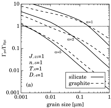
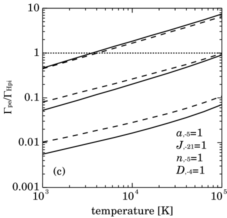
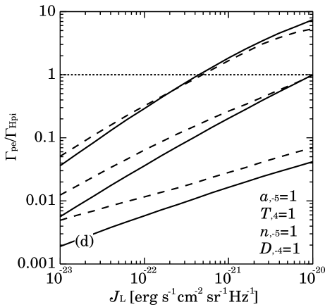
Figure 12: Ratio of dust photoelectric heating rate to hydrogen photoionization heating rate as a function of (a) grain size, (b) gas number density, (c) gas temperature, and (d) mean intensity at the Lyman limit. Notations are the same as figure A1. Additional parameter, $\cal D$ is the dust-to-gas mass ratio; ${\cal D}_{,-4}={\cal D}/10^{-4}$.

A.1 Analytic investigation

To understand the behavior of grain charge and other quantities found in figures A1–A3 analytically, we will adopt some further approximations in this subsection which do not appear in the method described in Inoue & Kamaya (2003). However, the method by Inoue & Kamaya (2003) is used in the calculation for making figures A1–A4 and in section 4. We would like to ask the reader to be careful in this point.

Let us express $eU/k_{\rm B}T$ as $x$. If we neglect the charging rate by grain–ion collision, the charge equilibrium is expressed as

$$s_{\rm e}n_{\rm e}\langle v_{\rm e}\rangle(1+x)=\int_{0}^{h\nu_{\rm max}}Q_{\nu}Y_{\nu}\frac{4\pi J_{\nu}}{h\nu}d\nu\,,$$ (10)

where $s_{\rm e}$ is the sticking coefficient for an electron collision, $n_{\rm e}$ is the electron number density, $\langle v_{\rm e}\rangle$ is the mean kinetic velocity of electron, $Q_{\nu}$ is the absorption efficiency factor of grains, $Y_{\nu}$ is the photoelectric yield, and $J_{\nu}$ is the mean intensity of the incident radiation. The left-hand side of the above equation is the electron capture rate per unit area, and the right-hand side is the photoelectric ionization rate per unit area. Although the integral should be summed up to infinity in general, we set the upper limit of the incident photon energy, $h\nu_{\rm max}=1.24$ keV. We also adopt $s_{\rm e}=1$.

In order to investigate analytically, we adopt a simple functional form for the photoelectric yield by Draine (1978);

$$Y_{\nu}=Y_{\infty}\left(1-\frac{I_{\rm p}}{h\nu}\right)$$ (11)

for $h\nu>I_{\rm p}$ and $Y_{\nu}=0$ for otherwise, where $I_{\rm p}$ is the ionization potential; $I_{\rm p}\simeq W+xk_{\rm B}T$ with $W$ being the work function. We note that a more realistic function of the photoelectric yield by Weingartner & Draine (2001b) is used in Inoue & Kamaya (2003) and in section 4. Moreover, we adopt an approximation form of the absorption efficiency factor as $Q_{\nu}\approx Q_{\rm L}(\nu/\nu_{\rm L})^{-\beta}$, where $\nu_{\rm L}$ is the Lyman limit frequency of hydrogen. For a grain larger than $\sim 0.1$ µm, $\beta\simeq 0$, and for a smaller grain, $\beta\simeq 1$–2 against ultraviolet photons. A power-law spectrum for the radiation, $J_{\nu}=J_{\rm L}(\nu/\nu_{\rm L})^{-\alpha}$ is also assumed.

If we define a function as $f(h\nu)=QYJ/h\nu$, $\partial f/\partial h\nu=0$ only when $h\nu=h\nu_{*}=I_{\rm p}(\alpha+\beta+2)/(\alpha+\beta+1)$. Because the function $f$ has the single peak at $h\nu_{*}$, the integral in equation (A1) is an order of $(4\pi/h)Q(h\nu_{*})Y(h\nu_{*})J(h\nu_{*})$. If $x\gg 1$, then, equation (A1) is reduced to

$$x^{1+\alpha+\beta}\sim\frac{4\pi Q_{\rm L}Y_{\infty}J_{\rm L}}{s_{\rm e}n_{\rm e}h(\alpha+\beta+2)}\left(\frac{\alpha+\beta+1}{\alpha+\beta+2}\right)^{\alpha+\beta}\left(\frac{h\nu_{\rm L}}{k_{\rm B}T}\right)^{\alpha+\beta}\left(\frac{\pi m_{\rm e}}{8k_{\rm B}T}\right)^{1/2}\,,$$ (12)

where we approximated $I_{\rm p}\approx xk_{\rm B}T$ because $W/k_{\rm B}T\sim 1$ for $T\sim 10^{4}$ K, and substituted $\langle v_{\rm e}\rangle=(8k_{\rm B}T/\pi m_{\rm e})^{1/2}$. If $n_{\rm e}\simeq n$ with $n$ being the gas number density, we find

$$\frac{eU}{k_{\rm B}T}\propto\left(\frac{J_{\rm L}Q_{\rm L}(a)}{n}\right)^{1/(1+\alpha+\beta)}T^{-(1/2+\alpha+\beta)/(1+\alpha+\beta)}\,.$$ (13)

Indeed, such dependences are found in figure A1. Moreover, $Q_{\rm L}\sim(a/0.1\micron)$ for $a\la 0.1$ µm and $Q_{\rm L}\sim 1$ otherwise. Thus, $eU/k_{\rm B}T$ shows nearly no dependence of grain size for a large size.

The mean photoelectron energy is defined as

$$\langle E_{\rm pe}\rangle=\frac{\int E_{\rm pe}Q_{\nu}Y_{\nu}4\pi J_{\nu}/h\nu d\nu}{\int Q_{\nu}Y_{\nu}4\pi J_{\nu}/h\nu d\nu}\,,$$ (14)

where $E_{\rm pe}$ is the energy of the photoelectron. We can express $E_{\rm pe}\approx\eta(h\nu-I_{\rm p})$, where $\eta$ is a numerical factor less than unity because a part of energy of the incident photon is converted into the phonon energy of the grain (Weingartner & Draine, 2001b). If we adopt a parabolic function for the energy distribution function of the photoelectron as Weingartner & Draine (2001b), the numerical factor $\eta=1/3$–1/2 depending on the energy of the incident photon. We adopt $\eta=1/2$ below.

If we define a function as $g(h\nu)=E_{\rm pe}QYJ/h\nu$ and assume the functional forms adopted above for $Q$, $Y$, and $J$, $\partial g/\partial h\nu$ is zero only when $h\nu=h\nu_{**}=I_{\rm p}(\alpha+\beta+2)/(\alpha+\beta)$. Thus, the integral in the numerator of equation (A5) is an order of $E_{\rm pe}(h\nu_{**})Q(h\nu_{**})Y(h\nu_{**})J(h\nu_{**})$. If $x\gg 1$, we obtain

$$\frac{\langle E_{\rm pe}\rangle}{xk_{\rm B}T}\sim\frac{2}{\alpha+\beta}\left(\frac{\alpha+\beta}{\alpha+\beta+1}\right)^{\alpha+\beta}\,.$$ (15)

Therefore, $\langle E_{\rm pe}\rangle/k_{\rm B}T$ has a similar parameter dependence to $eU/k_{\rm B}T$, which is observed in figure A2.

The saturation of $\langle E_{\rm pe}\rangle/k_{\rm B}T$ is seen in the case of $\alpha=1$ for a lower density in figure A2 (b). This may be due to the effect of the maximum photon energy assumed in the calculation. We do not consider the incident photon energy higher than 1.2 keV. For the case, $I_{\rm p}$ reaches several hundreds eV, so that the peak energy $h\nu_{**}$ becomes nearly the maximum energy. Thus, the above estimate may be an overestimate for such a case.

The total photoelectric heating by dust is given by $\Gamma_{\rm pe}=n_{\rm d}\gamma$, where $n_{\rm d}$ is the grain number density and $\gamma$ is the heating rate per a grain. While $n_{\rm d}\propto na^{-3}$ for a certain dust-to-gas ratio, $\gamma$ is proportional to $\langle E_{\rm pe}\rangle a^{2}nT^{1/2}x$ because the photoelectric ionization rate per a grain balances with the electron capture rate per a grain, where $a^{2}$ dependence comes from the geometrical cross section of grains. We have assumed $x\gg 1$ again. On the other hand, the photoionization heating rate, $\Gamma_{\rm Hpi}$, is proportional to $n^{2}T^{-0.7}$ in the photoionization equilibrium, where the temperature dependence comes from the recombination coefficient. Therefore, we find

$$\frac{\Gamma_{\rm pe}}{\Gamma_{\rm Hpi}}\propto a^{-1}x^{2}T^{2.2}\,,$$ (16)

where we have used the relation $\langle E_{\rm pe}\rangle\propto xT$ (equation [A6]). Remembering $J$, $n$, and $T$ dependences in $x$ described in equation (A4), we can understand $J$, $n$, and $T$ dependences shown in figures A3 (b), (c), and (d). Because $Q_{\rm L}\propto a$ for $a\la 0.1$ µm and $Q_{\rm L}\sim 1$ for otherwise, we see a double power-law dependence of $a$ in panel (a) of figure A3.

A.2 Effect of the spectral break

As shown by Haardt & Madau (1996), the real spectrum may show a break at the He II Lyman limit (54.4 eV), whereas we have assumed a spectrum without break. Here this point is discussed. Assuming the power-law spectral index ($\alpha$) is fixed all over the spectral range for simplicity, we multiply the intensity of the background radiation above the He II Lyman limit by a factor of $f_{\rm HeII}$, which is called the spectral break factor in this appendix. As extreme cases, $f_{\rm HeII}=1$ means that there is no break, and $f_{\rm HeII}=0$ means that there is no photon above the He II Lyman limit. In all calculations, except for figure A4, $f_{\rm HeII}=1$ has been assumed.

Figure A4 shows the effect of $f_{\rm HeII}$ on the normalized mean photoelectron energy from dust grains ($\langle E_{\rm pe}\rangle/k_{\rm B}T$), which indicates the heating efficiency per a grain. Only the silicate case is shown, but the graphite case is very similar. For $\alpha=1$ case (dotted curves), we observe the photoelectron energy $\langle E_{\rm pe}\rangle/k_{\rm B}T$ decreases with decreasing $f_{\rm HeII}$. This is because the number of high energy photons decreases if the spectral break is larger (i.e. smaller $f_{\rm HeII}$). According to figure 5 in Haardt & Madau (1996), the break is significant like $f_{\rm HeII}\sim 0.1$. One might think that our assumption of $f_{\rm HeII}=1$ with $\alpha=1$ results in an overestimation of the dust heating, so that a larger amount of dust may be allowed in the IGM.

However, figure 5 of Haardt & Madau (1996) also shows that the spectral index is 0.5 rather than unity for $\la 1$ keV photons which we are interested in. In the $\alpha=0.5$ case (solid curves of figure A4), we find a good quantitative agreement with the case of $f_{\rm HeII}=1$ and $\alpha=1$ (top dotted curve) if $f_{\rm HeII}=0.1$–0.3. Therefore, our results obtained from the background spectrum of $f_{\rm HeII}=1$ and $\alpha=1$ should be quantitatively very consistent with those from a more realistic spectrum with the He II Lyman limit break.

Figure 13: Effect of the spectral break at the He II Lyman limit (54.4 eV) for silicate grains. Solid and dotted curves are the spectral index $\alpha=0.5$ and 1 cases, respectively. For each type of curves, we assume the spectral break factor, $f_{\rm HeII}=0.1$, 0.3, and 1 (no break) from bottom to top, respectively. The gas density $n_{,-5}=n/10^{-5}\,{\rm cm}^{-3}$, the gas temperature $T_{,4}=T/10^{4}\,{\rm K}$, and the intensity of the incident radiation $J_{,-21}=J_{\nu_{\rm L}}/10^{-21}\,{\rm erg\,s^{-1}\,cm^{-2}\,sr^{-1}\,Hz^{-1}}$ are assumed.

Appendix B Chemical rate equations and coefficients

In this paper, we consider HI, HII, HeI, HeII, HeIII, and electron as gaseous species. That is, we neglect the effect of the metal production by stars. The primordial helium mass fraction $Y=0.24$ is always adopted throughout our calculation.

Let us define a non-dimensional number abundance of each gaseous species as

$$X_{i}\equiv\frac{n_{i}}{n_{\rm b}}\,,$$ (17)

where $n_{i}$ is the number density of $i$-th species, and $n_{\rm b}$ is the baryon number density, which is given by $n_{\rm b}(z)=\Omega_{\rm b}\rho_{\rm c,0}(1+z)^{3}/\mu$ with $\rho_{\rm c,0}$ being the local critical density, and $\mu$ being the mean mass of baryon particles. Baryon is assumed to be only hydrogen and helium. Using the helium mass fraction $Y$, hence, we obtain

$$X_{\rm HI}+X_{\rm HII}=\frac{4(1-Y)}{4-3Y}\,,$$ (18)

$$X_{\rm HeI}+X_{\rm HeII}+X_{\rm HeIII}=\frac{Y}{4-3Y}\,,$$ (19)

and

$$\mu=\left(\frac{4}{4-3Y}\right)m_{\rm p}\,,$$ (20)

where $m_{\rm p}$ is the proton mass. For electron abundance, we have

$$X_{\rm e}=X_{\rm HII}+X_{\rm HeII}+2X_{\rm HeIII}\,.$$ (21)

Chemical rate equations for the gaseous species are

$$\frac{dX_{\rm HI}}{dt}=X_{\rm HII}X_{\rm e}n_{\rm b}\alpha_{\rm HII}-X_{\rm HI}(X_{\rm e}n_{\rm b}\beta_{\rm HI}+\gamma_{\rm HI})\,,$$ (22)

$$\frac{dX_{\rm HeI}}{dt}=X_{\rm HeII}X_{\rm e}n_{\rm b}\alpha_{\rm HeII}-X_{\rm HeI}(X_{\rm e}n_{\rm b}\beta_{\rm HeI}+\gamma_{\rm HeI})\,,$$ (23)

and

$$\frac{dX_{\rm HeIII}}{dt}=-X_{\rm HeIII}X_{\rm e}n_{\rm b}\alpha_{\rm HeIII}+X_{\rm HeII}(X_{\rm e}n_{\rm b}\beta_{\rm HeII}+\gamma_{\rm HeII})\,,$$ (24)

where $\alpha_{i}$, $\beta_{i}$, and $\gamma_{i}$ are recombination coefficients, collisional ionization coefficients, and photoionization rates for $i$-th species, respectively. The adopted functions of $\alpha_{i}$ and $\beta_{i}$ are tabulated in Table B1. The photoionization rate is given by

$$\gamma_{i}=\int_{\nu_{i}}^{\nu_{\rm max}}\sigma_{i,\nu}\frac{4\pi J_{\nu}}{h\nu}d\nu\approx\frac{4\pi}{h}\sigma_{i}J_{\rm L}\left(\frac{\nu_{\rm L}}{\nu_{i}}\right)^{\alpha}\left(\frac{b_{i}}{\alpha+s_{i}}-\frac{b_{i}-1}{\alpha+s_{i}+1}\right)\,,$$ (25)

where $J_{\nu}=J_{\rm L}(\nu/\nu_{\rm L})^{-\alpha}$ with $\nu_{\rm L}$ is the hydrogen Lyman limit frequency, and $\sigma_{i,\nu}$ is the ionization cross section:

$$\sigma_{i,\nu}=\sigma_{i}\left[b_{i}\left(\frac{\nu}{\nu_{i}}\right)^{-s_{i}}+(1-b_{i})\left(\frac{\nu}{\nu_{i}}\right)^{-s_{i}-1}\right]\,,$$ (26)

for $\nu\geq\nu_{i}$ and otherwise $\sigma_{i,\nu}=0$ (Osterbrock, 1989). The parameters for ionization cross sections are summarised in Table B2. The last term in equation (B9) is valid when $\nu_{\rm max}\gg\nu_{i}$. In this paper, we set $h\nu_{\rm max}=1.24$ keV.

Table 2: Recombination and collisional ionization coefficients in cm³ s^-1 taken from Cen (1992) and Theuns et al. (1998).

Recombination

$\alpha_{\rm HII}=6.30\times 10^{-11}T^{-1/2}T_{3}^{-0.2}/(1+T_{6}^{0.7})$

$\alpha_{\rm HeII}=1.50\times 10^{-10}T^{-0.6353}+\alpha_{\rm HeII}^{\rm D}$

$\alpha_{\rm HeIII}=3.36\times 10^{-10}T^{-1/2}T_{3}^{-0.2}/(1+T_{6}^{0.7})$

Dielectric recombination

$\alpha_{\rm HeII}^{\rm D}=1.9\times 10^{-3}T^{-1.5}e^{-4.7\times 10^{5}/T}(1+0.3e^{-9.4\times 10^{4}/T})$

Collisional ionization

$\beta_{\rm HI}=5.85\times 10^{-11}T^{1/2}(1+T_{5}^{1/2})^{-1}e^{-157809.1/T}$

$\beta_{\rm HeI}=2.38\times 10^{-11}T^{1/2}(1+T_{5}^{1/2})^{-1}e^{-285335.4/T}$

$\beta_{\rm HeII}=5.68\times 10^{-12}T^{1/2}(1+T_{5}^{1/2})^{-1}e^{-631515/T}$

Table 3: Parameters for ionization cross sections from Osterbrock (1989).

species	$\sigma_{i}$ [$10^{-18}$ cm2]	$\nu_{i}$ [$10^{15}$ Hz]	$b_{i}$	$s_{i}$
HI	6.30	3.29	1.34	2.99
HeI	7.83	5.94	1.66	2.05
HeII	1.58	13.2	1.34	2.99

By solving equations (B6)–(B8), we obtain $X_{\rm HI}$, $X_{\rm HeI}$, and $X_{\rm HeIII}$. Once these fractional abundances are obtained, other abundances are found from equations (B2), (B3), and (B5). In addition, the numbers of hydrogen and helium nuclei are constant since the helium mass fraction $Y$ is now constant. Thus, $dX_{\rm HII}/dt=-dX_{\rm HI}/dt$ and $dX_{\rm HeII}/dt=-dX_{\rm HeI}/dt-dX_{\rm HeIII}/dt$. Therefore, the term of $dX/dt$ in equation (6) of section 4.1 is reduced to $-dX_{\rm HI}/dt-dX_{\rm HeI}/dt+dX_{\rm HeIII}/dt$ because of $dX/dt=\sum_{i}dX_{i}/dt=dX_{\rm e}/dt$ and equation (B5).

We now consider the atomic photoionization heating and the photoelectric heating by dust as the heating mechanism of gas in equation (6). The photoionization heating rate per a $i$-th species atom/ion is given by

$$\epsilon_{i}=\int_{\nu_{i}}^{\nu_{\rm max}}(h\nu-h\nu_{i})\sigma_{i,\nu}\frac{4\pi J_{\nu}}{h\nu}d\nu\approx 4\pi\sigma_{i}\nu_{i}J_{\rm L}\left(\frac{\nu_{\rm L}}{\nu_{i}}\right)^{\alpha}\left(\frac{b_{i}}{\alpha+s_{i}-1}-\frac{2b_{i}-1}{\alpha+s_{i}}+\frac{b_{i}-1}{\alpha+s_{i}+1}\right)\,,$$ (27)

where parameters, $\sigma_{i}$, $\nu_{i}$, $b_{i}$, and $s_{i}$ are summarised in Table B2, and $\alpha$ is the power-law spectral index of the incident radiation. Again, the last term of equation (B11) is valid when $\nu_{\rm max}\gg\nu_{i}$. The dust photoelectric heating is given by calculating the equilibrium charge and the ejection rate of the photoelectron by the manner described in Inoue & Kamaya (2003). Finally, the adopted cooling rates are summarised in Table B3. The metallic line cooling is not so important for our problem because the temperature interested is less than 25,000 K and the metallicity is 1/10–1/100 of the Solar value (Sutherland & Dopita, 1993).

Table 4: Cooling coefficients in erg cm³ s^-1 taken from Cen (1992), Theuns et al. (1998), and Inoue & Kamaya (2003).

Recombination cooling
HII	$8.70\times 10^{-27}T^{1/2}T_{3}^{-0.2}/(1+T_{6}^{0.7})X_{\rm e}X_{\rm HII}$
HeII	$1.55\times 10^{-26}T^{0.3647}X_{\rm e}X_{\rm HeII}$
HeIII	$3.48\times 10^{-26}T^{1/2}T_{3}^{-0.2}/(1+T_{6}^{0.7})X_{\rm e}X_{\rm HeIII}$
dust	$(3/2)k_{\rm B}TR_{\rm e}n_{\rm d}/n_{\rm b}^{2}$
Dielectric recombination cooling
HeII	$1.24\times 10^{-13}T^{-1.5}e^{-4.7\times 10^{5}/T}(1+0.3e^{-9.4\times 10^{4}/T})X_{\rm e}X_{\rm HeII}$
Collisional ionization cooling
HI	$1.27\times 10^{-21}T^{1/2}(1+T_{5}^{1/2})^{-1}e^{-157809.1/T}X_{\rm e}X_{\rm HI}$
HeI	$9.38\times 10^{-22}T^{1/2}(1+T_{5}^{1/2})^{-1}e^{-285335.4/T}X_{\rm e}X_{\rm HeI}$
HeII	$4.95\times 10^{-22}T^{1/2}(1+T_{5}^{1/2})^{-1}e^{-631515/T}X_{\rm e}X_{\rm HeII}$
Collisional excitation cooling
HI	$7.5\times 10^{-19}(1+T_{5}^{1/2})^{-1}e^{-118348/T}X_{\rm e}X_{\rm HI}$
HeII	$5.54\times 10^{-17}T^{-0.397}(1+T_{5}^{1/2})^{-1}e^{-47638/T}X_{\rm e}X_{\rm HeII}$
Bremsstrahlung cooling
ion	$1.42\times 10^{-27}g_{\rm f}T^{1/2}X_{\rm e}(X_{\rm HII}+X_{\rm HeII}+4X_{\rm HeIII})$
Inverse compton cooling
CMB photon	$5.406\times 10^{-36}[T-T_{\rm CMB}(1+z)](1+z)^{4}X_{\rm e}/n_{\rm b}$

References

- Aguirre (1999) Aguirre, A., 1999, ApJ, 525, 583
- Aguirre & Haiman (2000) Aguirre, A., & Haiman, Z., 2000, ApJ, 532, 28
- Aguirre et al. (2001) Aguirre, A., Hernquist, L., Katz, N., Gardner, J., & Weinberg, D., 2001, ApJ, 556, L11
- Aguirre et al. (2004) Aguirre, A., Schaye, J., Kim, T.-S., Theuns, T., Rauch, M., & Sargent, W. L. W., 2004, ApJ, in press
- Barger, Cowie, & Richards (2000) Barger, A. J., Cowie, L. L., & Richards, E. A., 2000, AJ, 119, 2092
- Bouwens et al. (2003) Bouwens, R. J., et al., 2003, ApJ, 595, 589
- Bromm, Yoshida, & Hernquist (2003) Bromm, V., Yoshida, N., & Hernquist, L. 2003, ApJ, 596, L135
- Buat et al. (2002) Buat, V., Boselli, A., Gavazzi, G., & Bonfanti, C., 2002, A&A, 383, 801
- Burstein & Heiles (1982) Burstein, D., & Heiles, C., 1982, AJ, 87, 1165
- Calzetti (2001) Calzetti, D., 2001, PASP, 113, 1449
- Cen (1992) Cen, R., 1992, ApJS, 78, 341
- Cheng, Gaskell, & Koratkar (1991) Cheng, F. H., Gaskell, C. M., & Koratkar, A. P., 1991, ApJ, 370, 487
- Connolly et al. (1997) Connolly, A. J., Szalay, A. S., Dickinson, M., Subbarao, M. U., & Brunner, R. J., 1997, ApJ, 486, L11
- Cowie et al. (1995) Cowie L. L, Songaila A., Kim T. S., & Hu E. M., 1995, AJ, 109, 1522
- Draine (1978) Draine, B. T., 1978, ApJS, 36, 595
- Draine & Lee (1984) Draine, B. T., & Lee, H. M., 1984, ApJ, 285, 89
- Draine & Sutin (1987) Draine, B. T., & Sutin, B., 1987, ApJ, 320, 803
- Draine & Hao (2002) Draine, B. T., & Hao, L., 2002, ApJ, 569, 780
- Dunne et al. (2003) Dunne, L., Eales, S., Ivison, R., Morgan, H., & Edmunds, M. 2003, Nature, 424, 285
- Elfgren & Désert (2003) Elfgren, E., & Désert, F.-X. 2003, A&A, submitted (astro-ph/0310135)
- Ferrara et al. (1990) Ferrara, A., Aiello, S., Ferrini, F., & Barsella, B., 1990, A&A, 240, 259
- Ferrara et al. (1991) Ferrara, A., Ferrini, F., Barsella, B., & Franco, J., 1991, ApJ, 381, 137
- Ferrara et al. (1999) Ferrara, A., Nath, B., Sethi, S. K., & Shchekinov, Y., 1999, MNRAS, 303, 301
- Gallego et al. (1995) Gallego, J., Zamorano, J., Aragon-Salamanca, A., & Rego, M., 1995, ApJ, 455, L1
- Giavalisco et al. (2004) Giavalisco, M., et al. 2004, ApJ, 600 L103
- Goobar, Bergstöm, & Mörtsell (2002) Goobar, A., Bergstöm, L., & Mörtsell, E., 2002, A&A, 384, 1
- Haardt & Madau (1996) Haardt, F., & Madau, P., 1996, ApJ, 461, 20
- Hui & Gnedin (1997) Hui, L., & Gnedin, N. Y., 1997, MNRAS, 292, 27
- Inoue (2003) Inoue, A. K., 2003, PASJ, 55, 901
- Inoue & Kamaya (2003) Inoue, A. K., & Kamaya, H., 2003, MNRAS, 341, L7
- Iwata et al. (2003) Iwata, I., Ohta, K., Tamura, N., Ando, M., Wada, S., Watanabe, C., Akiyama, M., & Aoki, K., 2003, PASJ, 55, 415
- Jaffe et al. (2001) Jaffe, A. H., et al., 2001, Phys.Rev.Lett., 86, 3475
- Kozasa & Hasegawa (1987) Kozasa, T., & Hasegawa, H. 1987, Prog. Theor. Phys., 77, 1402
- Laor & Draine (1993) Laor, A., & Draine, B. T., 1993, ApJ, 402, 441
- Lilly et al. (1996) Lilly, S. J., Le Fevre, O., Hammer, F., & Crampton, D., 1996, ApJ, 461, L1
- Loeb & Haiman (1997) Loeb, A., & Haiman, Z., 1997, ApJ, 490, 571
- Madau et al. (1996) Madau, P., Ferguson, H. C., Dickinson, M. E., Giavalisco, M., Steidel, C. C., & Fruchter, A., 1996, MNRAS, 283, 1388
- Madau, Pozzetti, & Dickinson (1998) Madau, P., Pozzetti, L., & Dickinson, M., 1998, ApJ, 498, 106
- Morgan et al. (2003) Morgan, H. L., Dunne, L., Eales, S., Ivison, R., & Edmunds, M. G. 2003, ApJ, 597, L33
- Mörtsell & Goobar (2003) Mörtsell, E., & Goobar, A., 2003, JCAP, 9, 9
- Nath, Sethi, & Shchekinov (1999) Nath, B. B., Sethi, S. K., & Shchekinov, Y., 1999, MNRAS, 303, 1
- Nozawa et al. (2003) Nozawa, T., Kozasa, T., Umeda, H., Maeda, K., & Nomoto, Ken’ichi 2003, ApJ, 598, 785
- Osterbrock (1989) Osterbrock, D. E. 1989, Astrophysics of Gaseous Nebulae and Active Galactic Nuclei (Mill Valley: University Science Books)
- Paerels et al. (2002) Paerels, F., Petric, A., Telis, G., & Helfand, D. J., 2002, BAAS, 201, 97.03
- Pagel (1997) Pagel, B. E. J., 1997, Nucleosynthesis and chemical evolution of galaxies (Cambridge: Cambridge University Press)
- Percival et al. (2001) Percival, W. J., et al., 2001, MNRAS, 327, 1297
- Perlmutter et al. (1999) Perlmutter, S., et al., 1999, ApJ, 517, 565
- Perna & Aguirre (2000) Perna, R., & Aguirre, A. 2000, ApJ, 543, 56
- Pryke et al. (2002) Pryke, C., et al., 2002, ApJ, 568, 46
- Riess et al. (1998) Riess, A. G., et al., 1998, AJ, 116, 1009
- Riess et al. (2001) Riess, A. G., et al., 2001, ApJ, 560, 49
- Rowan-Robinson, Negroponte, & Silk (1979) Rowan-Robinson, M., Negroponte, J., & Silk, J., 1979, Nature, 281, 635
- Schaye et al. (2000) Schaye, J., Theuns, T., Rauch, M., Efstathiou, G., & Sargent, W. L. W., 2000, MNRAS, 318, 817
- Schaye et al. (2003) Schaye, J., Aguirre, A., Kim, T.-S., Theuns, T., Rauch, M., & Sargent, W. L. W., 2003, ApJ, 596, 768
- Schlegel, Finkbeiner, & Davis (1998) Schlegel, D. J., Finkbeiner, D. P., & Davis, M., 1998, ApJ, 500, 525
- Schneider, Ferrara, & Salvaterra (2003) Schneider, R., Ferrara, A., & Salvaterra, R. 2003, MNRAS, submitted (astro-ph/0307087)
- Scott et al. (2002) Scott, J., Bechtold, J., Morita, M., Dobrzycki, A., & Kulkarni, V. P., 2002, ApJ, 571, 665
- Songaila (2001) Songaila, A. 2001, ApJ, 561, L153
- Spergel et al. (2003) Spergel, D. et al., 2003, ApJS, 148, 175
- Spitzer (1978) Spitzer, L., 1978, Physical Processes in the Interstellar Medium, Wiley, New York
- Springel & Hernquist (2003) Springel, V., & Hernquist, L., 2003, MNRAS, 339, 312
- Steidel et al. (1999) Steidel, C. C., Adelberger, K. L., Giavalisco, M., Dickinson, M., & Pettini, M., 1999, ApJ, 519, 1
- Sutherland & Dopita (1993) Sutherland, R. S., & Dopita, M. A., 1993, ApJS, 88, 253
- Takase (1972) Takase, B. 1972, PASJ, 24, 295
- Telfer et al. (2002) Telfer, R. C., Kriss, G. A., Zheng, W., Davidsen, A. F., & Tytler, D., 2002, ApJ, 579, 500
- Telis et al. (2002) Telis, G. A., Petric, A., Paerels, F., & Helfand, D. J., 2002, BAAS, 201, 79.12
- Theuns et al. (1998) Theuns, T., et al., 1998, MNRAS, 301, 478
- Theuns et al. (2002a) Theuns, T., et al., 2002a, ApJ, 574, L111
- Theuns et al. (2002b) Theuns, T., et al., 2002b, ApJ, 567, L103
- Todini & Ferrara (2001) Todini, P., & Ferrara, A., 2001, MNRAS, 325, 726
- Tresse & Maddox (1998) Tresse, L., & Maddox, S. J., 1998, ApJ, 495, 691
- Weingartner & Draine (2001a) Weingartner, J. C., & Draine, B. T., 2001a, ApJ, 548, 296
- Weingartner & Draine (2001b) Weingartner, J. C., & Draine, B. T., 2001b, ApJS, 134, 263
- Whittet (2003) Whittet, D. C. B., 2003, Dust in the Galactic Environment 2nd edition (Bristol: Institute of Physics)
- Windt (2002) Windt, D. L. 2002, ApJ, 564, L61
- Wright (1981) Wright, E. L., 1981, ApJ, 250, 1
- Zheng et al. (1997) Zheng, W., Kriss, G. A., Telfer, R. C., Grimes, J. P., & Davidsen, A. F., 1997, ApJ, 475, 469