An ultraviolet-selected galaxy redshift survey - III: Multicolour imaging and non-uniform star formation histories

Abstract

We present panoramic $u$’ and optical ground-based imaging observations of a complete sample of low-redshift ($0<z<0.4$) galaxies selected in the ultraviolet (UV) at 2000 Å using the balloon-borne FOCA instrument of Milliard et al. This survey is highly sensitive to newly-formed massive stars, and hence to actively star-forming galaxies. We use the new data to further investigate the optical, stellar population and star formation properties of this unique sample, deriving accurate galaxy types and $k$-corrections based on the broad-band spectral energy distributions.

When combined with our earlier spectroscopic surveys, these new data allow us to compare star-formation measures derived from aperture-corrected H$\alpha$ line fluxes, UV(2000 Å) and $u$’(3600 Å) continuum fluxes on a galaxy-by-galaxy basis. As expected from our earlier studies, we find broad correlations over several decades in luminosity between the different dust-corrected star-formation diagnostics, though the scatter is larger than that from observational errors, with significant offsets from trends expected according to simple models of the star-formation histories (SFHs) of galaxies. Popular galaxy spectral synthesis models with varying metallicities and/or initial mass functions seem unable to explain the observed discrepancies.

We investigate the star-formation properties further by modelling the observed spectroscopic and photometric properties of the galaxies in our survey. We find that nearly half of the galaxies surveyed possess features that appear incompatible with simple constant or smoothly declining SFHs, favouring instead irregular or temporally-varying SFHs. We demonstrate how this can reconcile the majority of our observations, enabling us to determine empirical corrections that can be used to calculate intrinsic star formation rates (as derived from H$\alpha$ luminosities) from measures based on UV (or $u$’) continuum observations alone. We discuss the broader implications of our finding that a significant fraction of star-forming galaxies have complex SFHs, particularly in the context of recent determinations of the cosmic SFH.

1 Introduction

An accurate determination of the star-formation history (SFH) of the Universe is one of the key goals of modern observational cosmology. Studies which measure, analyse and model its precise form are important not only in indicating likely epochs of dominant activity, but also for comparisons with the predictions of semi-analytical models of galaxy formation, and as such have provided a major impetus towards a fuller understanding of the physical mechanisms of galaxy evolution.

Various techniques now exist to measure star-formation rates (SFRs) in distant galaxies, all of which are sensitive in some way to the number of young, short-lived, and hence massive stars. These include nebular recombination (e.g. H$\alpha$) and forbidden line (e.g. [O ii]) emission (Kennicutt, 1983; Gallagher et al., 1989; Gallego et al., 1995; Tresse et al., 2002; Hippelein et al., 2003), ultraviolet (UV) continuum measures in the wavelength range 1500 to 2800 Å (Donas et al., 1987; Lilly et al., 1996; Connolly et al., 1997; Treyer et al., 1998; Cowie et al., 1999; Sullivan et al., 2000; Wilson et al., 2002), decimetric radio emission (Condon, 1992; Cram et al., 1998; Haarsma et al., 2000), and far-infrared continuum emission (Rowan-Robinson et al., 1997; Blain et al., 1999; Kewley et al., 2002) (for a review of these techniques and their associated uncertainties, see Kennicutt, 1998). Currently, many of these diagnostics are only available over limited (and sometimes non-overlapping) redshift ranges, so studies of the evolution of the cosmic SFH have tended to combine many disparate studies measuring star-formation using a selection of the techniques described above, without an accurate understanding of how underlying physical processes in galaxies can affect different diagnostics.

However, there has been recent progress in inter-comparing and calibrating these measures by investigating the degree to which the different diagnostics agree when measured for the same galaxies. Work to date comparing H$\alpha$/UV measures (Glazebrook et al., 1999; Sullivan et al., 2000; Hopkins et al., 2001; Bell & Kennicutt, 2001; Buat et al., 2002) and radio/H$\alpha$/UV measures (Cram et al., 1998; Hopkins et al., 2001; Sullivan et al., 2001) has revealed broad correlations but with a significant scatter, together with some offsets from relations expected from simple SFH scenarios. Such discrepancies indicate either poorly understood dust extinction corrections (particularly on UV measures), some physical parameter varying from galaxy to galaxy, such as the metallicity or initial mass function, or variations in the timescale of recent star-formation and consequent contamination of UV-continuum derived SFRs by older and less massive stars.

We have been using a unique sample of local UV-selected galaxies to investigate these issues, constructed using the balloon-borne camera of Milliard et al. (1992) which images the sky at 2000 Å. In Treyer et al. (1998) we used this sample to construct the first local UV luminosity function, finding an integrated star-formation density higher than that found in local emission-line surveys. Sullivan et al. (2000) extended this sample, and performed initial investigations into the physical nature of star-formation in the sample comparing H$\alpha$ and UV-derived SFRs. Evidence for non-linearities and significant scatter was found, though questions over aperture corrections on the H$\alpha$ measures and $k$-corrections on the UV luminosities remained. The radio properties (Sullivan et al., 2001) and chemical properties (Contini et al., 2002) of this sample have also been investigated.

In this paper, we further constrain the nature of star-formation in the sample. We extend our previous studies to include new broad-band $u$’ and optical $Br^{\prime}$ imaging observations of a substantial fraction of the galaxies in the survey, allowing accurate aperture and $k$-corrections to be made. We then use the combined samples to investigate the optical and stellar population properties of the sample, as well as to investigate SFRs derived from a second UV continuum measure in conjunction with that previously measured at 2000 Å.

An outline of the paper is as follows. In Section 2 we introduce the redshift survey data, including the new imaging campaigns. Section 3 discusses the optical properties of the sample, allowing improved aperture and $k$-corrections for our spectroscopic data. Section 4 then examines the star-formation properties of the galaxies derived from H$\alpha$/UV/$u$’ observations. We model and discuss the implications of our results in Section 5, and conclude in Section 6. Throughout this paper we assume a $\Omega_{\Lambda}=0.7$, $\Omega_{\mathrm{M}}=0.3$, $h=0.70$ (where $H_{0}=100\,h\,\mathrm{km\,s^{-1}\,Mpc}^{-1}$) cosmology.

2 The Survey Datasets

This paper extends our earlier work of Treyer et al. (1998, hereafter T98) and Sullivan et al. (2000, hereafter S2000) by augmenting our photometric dataset with with more extensive and precise optical photometry. Here, we introduce the new datasets which are analysed in this paper. We commence with a brief discussion of the existing datasets – UV imaging data taken from the FOCA experiment and the follow-up optical spectroscopy – followed by the details of the new imaging surveys of these fields.

2.1 The FOCA redshift survey

The FOCA instrument is a balloon-borne 40-cm Cassegrain with a single filter approximating a Gaussian centred at 2015Å, FWHM 188Å (Milliard et al., 1992). Two fields observed by FOCA are studied here: the high galactic-latitude region of Selected Area 57 (SA57; $\mathrm{RA}=13^{\mathrm{h}}06^{\mathrm{m}}10\aas@@fstack{s}43$, $\mathrm{Dec.}=+29\degr 01\arcmin 46\aas@@fstack{\prime\prime}1$, J2000) and the field of the $z=0.0215$ Leo cluster, Abell 1367 (A1367; $\mathrm{RA}=11^{\mathrm{h}}45^{\mathrm{m}}20\aas@@fstack{s}92$, $\mathrm{Dec.}=+19\degr 53\arcmin 23\aas@@fstack{\prime\prime}0$, J2000). The UV exposure times corresponded to a limiting magnitude of $m_{\mathrm{U}V}=18.5$ in the FOCA photometric system ($m_{\mathrm{U}V}^{\mathrm{A}B}\simeq 20.75$). Both fields have extensive multi-fibre optical spectroscopy obtained using the WIYN/Hydra (3500 – 6600 Å; 3.1-arcsec diameter fibres) and WHT/WYFFOS (3500 – 9000 Å; 2.7-arcsec diameter fibres) telescope/instrument combinations, providing redshifts for 224 UV-selected emission-line galaxies, of which H$\alpha$ fluxes can be reliably measured in 111 objects. The wavelength coverage of the WIYN data preclude observation of H$\alpha$. Fluxes, equivalent widths (EWs), and errors for each of the principle emission lines, as well as the strength of the 4000 Å Balmer break (D4000; see e.g. Bruzual, 1983), are measured where the signal-to-noise (S/N) of the spectra permits. Where H$\alpha$ is not detected, an upper flux limit is estimated at the emission wavelength using the noise characteristics of each spectrum.

The Balmer emission lines are corrected for the effects of stellar absorption as described in earlier papers (S2000), with a median correction of 2.5 Å. Fluxes are also corrected for the effects of Galactic extinction using the dust maps of Schlegel et al. (1998) and a Cardelli et al. (1989) extinction law. These corrections are small, with typical $E(B-V)$s of 0.01 and 0.02 for SA57 and A1367 respectively. The ratio of these corrected H$\alpha$ and H$\beta$ fluxes is used to determine the colour excess of the ionised gas, $E(B-V)_{\mathrm{g}}$, and hence the internal dust extinction assuming case-B recombination and a Cardelli et al. (1989) attenuation law. AGN and QSO-like objects are removed from the star-forming sample on the basis of their optical spectra (objects with broad emission lines are discarded). Of the remaining narrow-band objects, the vast majority are star-forming galaxies, as evidenced from diagnostic diagrams based upon the ratios of their principle emission lines (Contini et al., 2002). Details of all these procedures can be found in Sullivan (2002).

2.2 Optical Imaging Campaigns

The new optical data are taken from three sources: A $u$’/$r$’ Palomar/LFC imaging programme of SA57, $B$-band imaging using the CFHT/12k camera, and supplementary $gri$ data from the Palomar Digital Sky Survey (DPOSS) for both SA57 and A1367.

2.2.1 The Palomar Large Format Camera

The Large Format Camera (LFC Simcoe et al., 2000) on the Palomar 200-in Hale telescope is a mosaic of six 2048x4096 pixel CCDs (though only four were available when the data for this paper were collected), covering a region of diameter $\sim 24$$\arcmin$ with a pixel scale of 0.175 arcseconds. Data were collected over the course of six dark nights split over two observing runs in April 2000 and March 2001. The 1.5$\degr$ diameter field of SA57 was mosaiced using Sloan Digital Sky Survey (SDSS) $u$’ and $r$’ filters, with a tessellation pattern avoiding bright foreground stars which created serious saturation and bleed trails on the LFC CCDs. Exposure times were 2400s in $u$’ and 600s in $r$’. Due to time constraints, we concentrated our observations on the centre of the SA57 field.

The LFC data were reduced using a hybrid of the National Optical Astronomy Observatories (NOAO) mosaic reduction software for use in iraf (Valdes, 1998) as well as custom-written routines to deal with some issues specific to the LFC. The data were bias-subtracted using the overscan regions on the chips and nightly master bias frames. Flat-fielding was performed using dome flats (for $r$’ data) and twilight sky flats (for $u$’ data) taken on each night. We also constructed a ‘super-sky’ flat for the $r$’ data by stacking all the $r$’ observations; however the resulting sky flat-field frame was virtually indistinguishable from the dome flat, and hence was not used. The iraf routine mscskysub was used to remove any second-order sky gradients across the field by computing medians in boxes of size 50 pixels and fitting a low-order two dimensional function to the median points. The residual ‘fitted-sky minus sky mean’ is subtracted from each pixel.

We derived astrometric solutions for each chip in the two filters using astrometric calibration exposures. SA57 is a (deliberately chosen) high galactic latitude field where the surface density of bright foreground galactic stars required for astrometric calibration is low. We therefore observed astrometric calibration fields taken from the Astrometric Calibration Regions (ACRs) catalogue of Stone et al. (1999), with star positions typically accurate to $\pm 26$ mas. We use sextractor (Bertin & Arnouts, 1996) and the WCSTools software suite written by D. Mink (e.g. Mink, 1999) to create approximate world co-ordinate system (WCS) solutions for each astrometric region in each filter based on stars in the ACR catalogues, discarding stars with large proper motions. The WCS was then refined using the iraf program ccmap and a TNX projection with a high order polynomial and half cross-terms. This flexible function was needed to fit the edges of the LFC chips where distortion can be significant. The plate solution for each filter/chip was then applied to every science exposure using the iraf mscred tasks, shifting the reference point for the plate solution for each science field using the USNO-A2.0 stars (i.e. there are enough of these stars to calculate a reference point shift, but not to derive a full plate solution). The final solution for each science field is accurate to 0.15 – 0.2″, even for the regions of the chips that suffer significant distortion.

Each exposure was projected and re-sampled onto a linear WCS, and the individual dither steps at each pointing median-combined after masking cosmic-rays and chip defects to create one final dithered image for each chip, applying multiplicative scaling factors to allow for airmass differences between dithers. The result is an astrometrically calibrated and photometrically stable combined science image.

At the time the observing program was carried out, the SDSS filters were ‘non-standard’, in the sense that few published calibration stars were available. To avoid complex colour terms needed to place our data on the standard $\alpha$-Lyrae photometric system, we used standard spectrophotometric stars to calibrate our data. On each night, two spectrophotometric standard stars were monitored at approximately two hour periods throughout the night to derive airmass-dependent extinction correction terms, augmented by dawn and dusk twilight observations of 4 – 5 other spectrophotometric standard stars. Our preferred standards were Feige 67 and Feige 34. We calculated the AB magnitude of each standard star in the $u$’ and $r$’ filters using the spectrophotometric star spectra energy distributions (SEDs) taken from Massey et al. (1988) and Massey & Gronwall (1990). We convolved these SEDs with the filter and LFC-CCD responses (C. Steidel, private communication) to calculate the magnitude in a particular filter.

The $r$’ zero-point was extremely stable with a mean r.m.s. dispersion of $\simeq 0.01$ mag. The $u$’ zero-point was less well-defined, with an r.m.s. variation from standard star to standard star of $\simeq 0.03$ mag. Due to the accuracy limit to which the spectra of these standard stars are calibrated an accuracy greater than 0.03 mag in $u$’ is probably not achievable (see e.g. Steidel & Hamilton, 1993). As an additional consistency check, the overlapping nature of the mosaicing technique allows us to compare magnitudes of objects in different fields, and a night-to-night (or even year-to-year) comparison is possible. We typically find agreement to within 0.02 mag in $r$’, rising to 0.04 mag for the $u$’ data. No offsets were seen between the same objects measured on different nights.

Object catalogues were created using sextractor version 2.2.2 (Bertin & Arnouts, 1996). We used the automatic aperture magnitudes determined by sextractor, similar to Kron’s ‘first moment’ algorithm (Kron, 1980). Our high galactic-latitude fields contain a low source-density of objects (particularly in $u$’), so crowding on the fields was not a problem and de-blending was rarely required.

2.2.2 CFHT and DPOSS data

A second optical survey of SA57 was conducted using the Canada France Hawaii Telescope (CFHT) and the CFH12k instrument, a large mosaicing camera with an imaging area of 42$\arcmin$$\times$28$\arcmin$ (see Cuillandre et al., 2000). The observations were carried out on the 25th (3/4 night) and 26th (1/4 night) May 2000 using seven CFHT12k pointings to cover the SA57 field. The first night was photometric, but poor weather on the second night curtailed the program. Each pointing comprised two 300s dithered exposures. Landolt (1992) standard star fields were interspersed with the science observations to achieve a photometric calibration of the data.

The data were reduced at the TERAPIX centre using the TERAPIX pipeline reduction software designed for use with the CFH12k camera according to a procedure described in the June 2002 TERAPIX progress report. An image catalogue covering SA57 was constructed using the sextractor package and here again we use the automatic aperture magnitudes. The catalogue is complete to $B=24$.

Finally, we augment the two dedicated observing programs of SA57 with data taken from the Digitised Palomar Sky Survey (DPOSS). This provides data for both SA57 and A1367 in $g$, $r$ and $i$ Gunn filters (see Gal et al., ????). The areal coverage in both fields is 100 per cent, though the data are shallower ($g<22.5$) and of limited photometric accuracy when compared to the Palomar/CFHT data, hence we use the DPOSS data where no other imaging is available. The optical sources in the various bands are uniquely matched within a search radius of 1.5″. As in our earlier papers, we use a search radius of 10″ to assign optical counterparts from our combined optical data to the FOCA sources. The problem of multiple optical counterparts is addressed in Section 3.1.

2.3 Comparing the magnitude systems

To consistently inter-compare these new photometric data, we place all the magnitudes onto a system with the same calibration zeropoint. Our imaging data comprises four different calibration systems: The FOCA system (e.g. Milliard et al., 1992), the Vega system (e.g. Johnson & Morgan, 1953; Fukugita et al., 1995), the AB system (e.g. Oke, 1974), and the Gunn system (e.g. Oke & Gunn, 1983). We compute conversions between the different systems using the SEDs of Vega, BD+17°4708 (for Gunn magnitudes), and appropriate filter and CCD response curves. Because of the advantages of a system where magnitudes are easy to interpret physically, we align all of our magnitudes onto the AB system, defined as:

$$m_{\nu}=-2.5\log(F_{\nu})-48.60$$ (1)

where $F$ is the flux in $\mathrm{erg}\,\mathrm{s}^{-1}\,\mathrm{cm}^{-2}\,\mathrm{Hz}^{-1}$. For convenience, we list the conversion values between the various original systems to the AB system in Table 1.

Table 1: Offsets used to convert the magnitudes to the AB system.

Filter	$\lambda_{\mathrm{eff}}$	Conversion from
	(Å)	${\mathrm{foca}}\rightarrow{\mathrm{AB}}$	${\mathrm{vega}}\rightarrow{\mathrm{AB}}$	${\mathrm{gunn}}\rightarrow{\mathrm{AB}}$
FOCA-UV	2015	+2.25
Palomar-$u$’	3603		+0.92
CFHT-$B$	4407		-0.10
DPOSS $g$	5330			+0.02
Palomar-$r$’	6282		+0.17
DPOSS $r$	6908			-0.19

3 Optical Properties

In this section we examine the photometric properties of the galaxy sample. We first describe our procedures for assigning optical counterparts to the FOCA source list, and then correct all of the observed magnitudes for the effect of internal dust extinction. The new optical coverage also allows us to estimate aperture corrections for our spectral measures, as well as a cross-check on the accuracy of the flux calibration of our spectra. We then continue with an exploration of the UV-optical properties, using the new data to derive improved galaxy types, $k$-corrections and luminosities compared to our earlier analyses.

3.1 FOCA – optical counterparts

One question remaining from our earlier papers concerned the number of FOCA detections with no apparent counterpart in optical data, which would imply either blue $UV-B$ colours or a number of false detections in the FOCA dataset. The optical imaging now available to us allows us to address this issue in a more comprehensive manner, as the depth of our $B$-band data is $\sim 2$ magnitudes deeper than the optical dataset used in S2000. This magnitude limit enables us to detect all the optical counterparts to the FOCA source list. We cross-correlate the combined optical $u^{\prime}Br^{\prime}$ catalogue with the FOCA source catalogue using a search radius of 10″ (see e.g. T98 or S2000 for details of the astrometric precision of the FOCA data). For each FOCA object, we record the number of matches, and assign each the nearest optical detection.

The number of multiple counterpart cases (where more than one optical detection lies within the search radius) is increased compared to S2000; however the number of UV detections with no optical counterpart is smaller: 50 per cent of the FOCA sources have multiple counterparts whilst less than 6 per cent have none. This 6 per cent thus represents a reasonable lower limit to the false detection rate in the FOCA source list, as the magnitude limit of the new data allows us to detect FOCA counterparts $\sim 1$ magnitude bluer in $UV-B$ than the bluest unreddened model starburst galaxy SED. The extra number of counterparts we find here are therefore most likely chance associations resulting from the higher surface density of objects in the fields: the brightest optical counterpart is also the closest in 85 per cent of the multiple counterpart cases. Where the brightest optical detection is more than 3 magnitudes brighter then the next brightest counterpart, we assume that the contribution to the UV flux of the fainter object is negligible and ignore it in our analyses. In our following analyses, ‘multiple optical counterparts’ galaxies are defined as those FOCA objects with two optical counterparts within $B$-band measures within 3 magnitudes of each other.

3.2 Dust and $k$-corrections

There are a variety of extinction laws (e.g., Milky Way, LMC, SMC) that could be used to apply the dust corrections factors derived from the Balmer decrements to the UV and optical magnitudes, giving quite different extinction corrections, particularly at UV wavelengths. The reddening of the UV continuum depends sensitively on the geometrical details of the dust-star-gas mix, with the reddening of the stellar continuum likely to be different to the obscuration of the ionised gas (derived empirically from the nebular emission via the Balmer decrement), as the stars and gas may occupy different areas within a galaxy with differing dust covering factors (see e.g. Fanelli et al., 1988; Calzetti et al., 1994; Mas-Hesse & Kunth, 1999). As in our previous work, we use the Calzetti et al. (2000) prescription, derived empirically from studies of local starburst galaxies, to ‘correct’ our optical fluxes. Calzetti et al. (2000) find that the colour excess of the stellar continuum, $E(B-V)_{\mathrm{s}}$, is related to the colour excess of the ionised gas, $E(B-V)_{\mathrm{g}}$, as $E(B-V)_{\mathrm{s}}=0.44\,E(B-V)_{\mathrm{g}}$.

We apply this reddening prescription to every filter passband in use in our survey using $E(B-V)_{\mathrm{g}}$ derived from the Balmer decrement. Where the H$\beta$ line is not detected, we use the SFR-dependent correction derived for this sample of galaxies presented in Sullivan et al. (2001) using an empirical SFR derived from the H$\alpha$ line (where both the H$\alpha$ and H$\beta$ lines are absent, we use the median $E(B-V)_{\mathrm{g}}$=0.3 representative of the whole sample). It is becoming apparent that luminosity-dependent dust corrections of this nature are not valid for star-formation across all Hubble types. However, for the mainly starburst or strongly star-forming galaxies typical in this sample, the luminosity dependent correction still appears an excellent approximation (Afonso et al., 2003).

We convert our observed (and dust-corrected) magnitudes, $m$, in the various passbands into rest-frame magnitudes by writing the corrected absolute magnitude, $M$, at $z=0$ as

$$M=m_{\mathrm{obs}}-5\log(\frac{D_{L}(z)}{10\,\mbox{pc}})-k(z)$$ (2)

where $D_{L}$ is the luminosity distance at redshift $z$, $m_{\mathrm{obs}}$ is the observed apparent magnitude, and $k(z)$ is the $k$-correction (see, for example, Yoshii & Takahara, 1988; Poggianti, 1997). We neglect any redshift-evolution in the physical properties of the galaxies in this calculation.

The magnitude of the $k$-corrections for template galaxy spectra using the range of the filters in this study strongly depends on galaxy type, with early-type galaxies (ellipticals and S0s) possessing larger $k$-corrections in the optical passbands than galaxies with flatter spectra. However, $k$-corrections in the FOCA passband are small with the largest $k$-corrections arising from elliptical and S0 type spectra, unlikely to be the predominant galaxy type in this UV-selected sample of objects.

We assign each object in our survey a $k$-correction by fitting the observed magnitudes to a set of model galaxy templates of varying type. Though we could do this by correlating our observed spectra with a set of template spectra, either via cross-correlation techniques (e.g. Connolly et al., 1995; Zaritsky et al., 1995; Heyl et al., 1997) or using a principal component analysis (see Folkes et al., 1999; Madgwick et al., 2002, and references therein), this approach requires spectra of a high S/N and wide wavelength coverage, which is not always the case in the spectra of our fainter objects. Instead, we use the popular technique of fitting a series of template SEDs to the broadband colours available for each galaxy and use the best-fitting SED for the estimation of $k$-corrections in each filter. This was also the approach used in T98 and S2000 though based on only a single $UV-b$ colour and using POSS-APM magnitudes, which have proved unreliable for bright galaxies. Here, we perform a more accurate calculation with the improved photometric coverage.

We determine our $k$-corrections by fitting each colour for a given galaxy to SED set, linearly interpolating between the SED types. These fits are combined by weighting inversely by the variance in the observed colours to obtain a mean best-fitting SED for each galaxy. For the dust-corrected colours we compare to the SEDs of Poggianti (1997) with 6 galaxy classes ranging from early-type galaxies (E/S0) to late-type spirals (Sc/Sd) supplemented with two starburst (SB) models, generated by superimposing a starburst on a passively evolving system (see T98 and S2000 for details). For our uncorrected colours we use the SEDs of Coleman et al. (1980), with 4 classes of SEDs from elliptical (E) to irregular (Im).

In Fig. 1, we present the results of the fitting process, showing the distribution of galaxy types ($T$) using each set of SEDs, with $T=1$ representing the reddest SED. The different classes are summarised in Table 2. Fig. 1 shows the majority of the galaxies are types Sb or later, with very few early-type objects. There is a good correspondence between the derived types (see Fig. 2), with the Poggianti (1997) derived types on average slightly bluer, possibly due to the inclusion of dust corrections in the derivation of these types. The mean types in each case are $T=3.15$ for the CWW SEDs ($\simeq$ Sd) and $T=6.43$ for the Poggianti SEDs ($\simeq$ Sd). No galaxies appear redder than the model SEDs, though at the blue end, 3 of the galaxies are bluer than the bluest CWW SED, whilst 2 are bluer than the bluest SB2 Poggianti SED. This points to a large population of actively star-forming or starbursting galaxies in the sample, as expected.

One caveat is that these galaxy types (and hence $k$-corrections) are based on the weighted average of (up to) four colours, and hence will not be sensitive to ‘peculiar’ colours in a single pair of filters where the other colours of that galaxy are ‘normal’. This might occur (for example) in a galaxy experiencing a sudden burst of star-formation; the $UV-B$ colours might appear very blue whilst the $B-r^{\prime}$ or $r-i$ colours could be almost unchanged from their pre-burst values. We return to this issue in later sections.

Table 2: The correspondence between the different galaxy classes.

SED set	E	S0	Sa	Sb	Sc	Sd	Im/SB1	SB2
Poggianti	1	2	3	4	5	6	7	8
CWW	1			2	3         4

Figure 1: The distribution of galaxy types ($T$) in our survey. UPPER: $T=1$ corresponds to an E SED, $T=8$ corresponds to an SB2 SED. SEDs from Poggianti (1997). LOWER: $T=1$ corresponds to an E SED, $T=4$ corresponds to an Im SED. SEDs are from Coleman et al. (1980).

Figure 2: Comparison of the galaxy types derived from the two SED sets, with the CWW SED types on the $x$-axis and the Poggianti SED types on the $y$-axis, demonstrating the agreement between the galaxy types derived from the two sets of SEDs, as well as before and after dust corrections have been applied. The stars show locations where the two types approximately correspond.

3.3 Aperture Corrections

In S2000, we saw that H$\alpha$ derived SFRs were generally smaller than UV-based SFRs by factors of around 3 – 4. Potential (non-physical) explanations of this effect could be related to uncertainties in the flux calibration of the spectral data, or if the 2.7″ diameter fibres used on the WYFFOS spectrograph were sampling only a small fraction of the total galaxy light, and hence generating an aperture mismatch when compared to the FOCA magnitudes. In S2000, we found little significant trend in the ratio of H$\alpha$/UV light with redshift (and hence apparent size), as would be expected if aperture corrections were not a significant source of uncertainty. However, the new $B$ and $r$’-band data allow us to address any remaining uncertainties, as well as to extend the number of objects in the survey with a calibrated H$\alpha$ measure.

For every FOCA $B$ and $r$’ counterpart, we measure from the imaging data the magnitude of each object inside a radius of 2.7″(the WYFFOS fibre radius) using sextractor. We convolve the flux-calibrated spectrum with the filter+CCD response of the $B$/$r$’ filters to generate corresponding ‘spectral magnitudes’. We find that the spectral $B$-$r$’ colours typically agree with the optical 2.7″ $B$-$r$’ colours to within 10-20 per cent, indicating little wavelength-dependent uncertainty in the flux calibration. We then calculate aperture corrections by comparing the $r$’ spectral magnitudes with the total $r$’ magnitude (as measured by sextractor), deriving correction factors by which we scale the H$\alpha$ fluxes. We see minor evidence for a magnitude dependent effect, with some apparently brighter, and likely nearer with a greater apparent size, objects requiring larger correction factors. We exclude galaxies which require very large corrections from our sample and the future analyses in this paper. The median factor for the survey is 1.26, i.e. 0.25 mag. For the small number of galaxies without any $r$’ information this median correction is applied. This median factor compares well with that derived by Tresse & Maddox (1998), who find a mean correction of 0.52 mag using $V$ band magnitudes for the CFRS galaxies, but with smaller 1.75″ slits, thus accounting for their slightly larger aperture corrections.

The $r$’-band data also allow us to apply a ‘flux calibration’ to H$\alpha$ fluxes which were taken during an observing run for which no standard stars were observed (detailed in T98), following a similar procedure as with the aperture corrections. This adds a further 17 objects to our H$\alpha$ sample.

These corrections assume that the H$\alpha$ emission in the galaxy is a uniform distribution, and that the galaxy is not dominated by either nuclear or disc star-formation. Whilst these uncertainties may be significant for local nearby objects (with a larger apparent size), by redshifts of 0.05 (i.e. for most of the galaxies in our sample) these effects are likely to be very small.

3.4 UV/Optical colours

One of the most puzzling features of the FOCA galaxies presented in our earlier papers was the presence of a sub-sample of galaxies with extremely blue $UV-B$ colours, bluer than most typical starburst SEDs. The improved optical data that we have assembled now allows us to examine the SEDs of these objects across a wider wavelength range.

With the new optical magnitudes, 8 and 5 per cent of the UV galaxies with a unique optical counterpart (slightly more when including multiple counterpart cases) are found to be bluer than the bluest Poggianti SED in $UV-B$ and $UV-g$ respectively (where the $g$ data also includes the A1367 field). Before dust correction, these fractions are $\simeq 4$ and $\simeq 2$ per cent respectively. At longer wavelengths, the galaxies have more ‘normal’ colours typical of the mean SED of the sample (see Fig. 3). As mentioned earlier, this might occur in galaxies experiencing a sudden burst of star-formation (see Section 5). A second possibility is that that hot Wolf-Rayet (WR) stars could be responsible for the UV excess as suggested by Brown et al. (2000). We examined this suggestion in detail in (Contini et al., 2002), studying the co-added spectrum of the bluest objects in the sample, but could identify no WR spectral features in the spectrum of galaxies with extreme $UV-B$ colours.

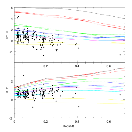
Figure 3: Colour-redshift distributions for the unique optical counterpart cases only. UPPER: $UV-B$, LOWER: $B-r$. The solid lines show the model predictions for the Poggianti (1997) set of SEDs, the dotted lines are the colours derived from the CWW SED’s (see text for details). The galaxies appear slightly bluer in $UV-B$ compared to the model SEDs than for $B-r$; additionally in $UV-B$ there is a small population of objects with colours bluer than the bluest model SED. The colours are in the AB system and are corrected for dust extinction.

4 Star-Formation properties of the Sample

We now turn to the main focus of this paper, continuing our investigations into the star-formation properties of the survey begun in S2000, where we examined the relationship between H$\alpha$ and UV derived SFRs. We found that this relationship possessed a scatter and non-unity best-fitting slope which could not be satisfactorily explained in scenarios assuming constant or other simple SFHs. We now use our new data to investigate these effects with increased precision.

4.1 Uncertainties in converting luminosities into star-formation rates

Our first step is to construct a framework within which we can transform our measured luminosities for each of the star-formation diagnostics into SFRs. As has been covered extensively in other studies, there are a remarkable number of free parameters in these models – the initial mass function (IMF), the stellar metallicity, and the choice of SED libraries, amongst many others (see Kennicutt, 1998, for a discussion of the issues). We derive conversion factors in a self-consistent manner using the pegase-ii spectral synthesis code (Fioc & Rocca-Volmerange, 1997, 1999). The three star-formation diagnostics available in this study are

• H$\alpha$ luminosity (L_Hα), originating from re-processed ionizing radiation at wavelengths $\lambda<912$ Å produced by the most massive ($>10\,\rm{M}_{\odot}$), short-lived ($\simeq 20\,\rm{Myr}$), OB-type stars. Accordingly, H$\alpha$ emission is a virtually instantaneous star-formation measure,reaching a constant level after $\simeq 10\,\rm{Myr}$ in a constant SFH. However, it is very sensitive to the form of the IMF due to the strong dependence on massive stars. Most calibrations assume case-B recombination (a comprehensive treatment of its use can be found in Charlot & Longhetti, 2001).

• UV 2000 Å continuum luminosity (L_UV), originating from stars spanning a range of ages (and hence initial masses), including some post-main sequence contribution. Hence, any L_UV to SFR calibration is dependent on the past history of star-formation, introducing a significant uncertainty when interpreting UV observations of star-forming galaxies. Dust corrections are also important in the UV, and a reliable correction can be difficult to achieve (e.g. Bell, 2002).

• $u$’ 3600 Å continuum luminosity (L${}_{u^{\prime}}$), with a similar physical origin as L_UV. The principle disadvantage is that $u$’ luminosities are contaminated by older, less massive stars to a greater extent than the UV-2000 Å data (given the longer wavelength), and this makes the calibration less certain than with shorter wavelength data. The advantage of using longer wavelengths is that dust corrections are smaller.

Using pegase-ii, we investigate the dependence of the three diagnostics to the principle free parameters in the spectral synthesis codes, varying each to determine the spread in the conversion values. We investigate metallicities of $Z=0.0004$, 0.004, 0.008, 0.02 ($=Z_{\odot}$) and 0.05, together with the IMFs of Salpeter (1955), Scalo (1998) and Kroupa (2001) using mass ranges of $0.1\rightarrow 100\,\mathrm{M}_{\odot}$, $0.1\rightarrow 120\,\mathrm{M}_{\odot}$, $0.1\rightarrow 50\,\mathrm{M}_{\odot}$, $1.0\rightarrow 100\,\mathrm{M}_{\odot}$ and $5.0\rightarrow 100\,\mathrm{M}_{\odot}$.

Table 3: Default conversions between luminosity and SFR

Tracer	Luminosity for $\mathrm{SFR}=1\,\mathrm{M}_{\odot}\,\mathrm{yr}^{-1}$
	$\mathrm{erg}\,\mathrm{s}^{-1}\,\mbox{\AA}^{-1}$	$\mathrm{erg}\,\mathrm{s}^{-1}\,\mathrm{Hz}^{-1}$
H$\alpha$	$1.22\times 10^{41}$ $\mbox{erg}\,\mbox{s}^{-1}$	—
UV 2000 Å	$5.75\times 10^{39}$	$7.78\times 10^{27}$
$u$’ 3600 Å	$1.71\times 10^{39}$	$7.40\times 10^{27}$

The uncertainties in the star-formation estimates due to these parameters are shown graphically in Fig. 4 as the distribution of L_Hα, L_UV and L${}_{u^{\prime}}$ and the distribution of the ratios of L_UV/L_Hα, L${}_{u^{\prime}}$/L_Hα and L${}_{u^{\prime}}$/L_UV for a constant SFR of 1 $\mathrm{M}_{\odot}\,\mathrm{yr}^{-1}$. There is a large spread in the conversion values for all diagnostics when considering the full range of IMFs and metallicities (around 1.5 orders of magnitude), with the importance of the timescale of recent star-formation for UV and $u$’ diagnostics clear. However, the scatter when considering the ratios of the diagnostics is much smaller, again with a strong time dependence. Though varying metallicities or IMFs can have a large effect on individual conversion values, the effects on the ratios is considerably smaller. Our default conversion values (listed in Table 3) assume solar metallicity, a Salpeter IMF with a mass range of 0.1 to 100 $\mathrm{M}_{\odot}$, and are taken 100 Myr into a constant SFH.

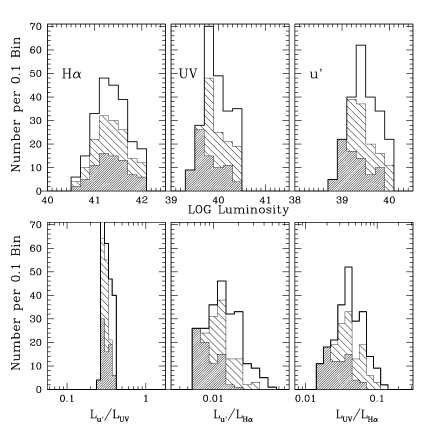
Figure 4: The distribution of the conversion values for the H$\alpha$, UV and $u$’ diagnostics (UPPER PANEL), and the distribution of the ratio of those values (LOWER PANEL), generated across the full range of metallicities, IMFs and mass ranges (see text for full details). The luminosities are those expected from star-formation rates of $1\,\mathrm{M}_{\odot}\,\mathrm{yr}^{-1}$. The shaded histograms refer to conversions taken at 10 (heavy shading), 100 (light shading) and 1000 Myr (no shading) in a constant SFH. The figure demonstrates how the ratios involving H$\alpha$ and UV (or $u$’) evolve according to the time after the onset of star-formation, whereas the ratio of $u$’/UV has little time dependence.

4.2 Comparing star-formation diagnostics

We present the relations between the different diagnostics in Fig. 5, showing comparisons between dust-corrected H$\alpha$, UV and $u$’ SFRs, overlaid with lines expected assuming constant star-formation and associated uncertainties in the position of this line derived from the analysis of the last section. Also shown are the error-weighted least-squares best-fits to the data. The H$\alpha$-UV plot is an updated version of fig. 13 in S2000 with the new aperture and $k$-corrections applied, together with some new measures and upper limits for H$\alpha$. Linear correlation (Pearson’s $r$) and Spearman rank-order correlation statistics, together with the weighted least-square best-fit equations and associated $\chi^{2}$, are presented in Table 4. We do not plot the relations before dust correction, and instead list the same statistical data for these samples in Table 4 as a comparison and so the effect of our dust-correction prescription can be seen.

Figure 5: A comparison of A) UV 2000 Å and H$\alpha$ SFRs, B) $u$’ 3600 Å and H$\alpha$ SFRs, C) UV 2000 Å and $u$’ 3600 Å, and D) the UV-B colour and the H$\alpha$ EW. All measures are dust corrected (and for H$\alpha$ aperture corrected) as described in the text. In the UV 2000 Å – $u$’ 3600 Åplot, galaxies possessing H$\alpha$ emission are marked as filled circles, those without as empty circles. The SFRs are calculated at 100 Myr into a constant SFH. The short-dashed lines denote an equality of SFRs and the long-dashed lines show typical uncertainties in the position of the short-dashed lines due to IMF/metallicity effects. Solid lines indicate weighted least-squares best-fits. In panel D), the overlaid lines correspond to the relation expected in a exponentially declining SFH for the three IMFs discussed in the text.

Table 4: The results for the various statistical tests for Fig. 5.

$\log(\mathrm{SFR})$	$N$	Pearson	Spearman	$\chi^{2}$	Equation
Relation
Corrected for dust:
H$\alpha$ – UV	106	0.918	0.916	348	$\log(\mathrm{SFR}_{\mathrm{uv}})=0.79\times\log(\mathrm{SFR}_{\mathrm{H}{\alpha}})+0.36$
H$\alpha$ – $u$’	78	0.909	0.906	793	$\log(\mathrm{SFR}_{u^{\prime}})=0.78\times\log(\mathrm{SFR}_{\mathrm{H}{\alpha}})+0.37$
$u$’ – UV	78	0.952	0.944	134	$\log(\mathrm{SFR}_{\mathrm{uv}})=1.13\times\log(\mathrm{SFR}_{u^{\prime}})-0.11$
Uncorrected:
H$\alpha$ – UV	106	0.889	0.887	391	$\log(\mathrm{SFR}_{\mathrm{uv}})=0.72\times\log(\mathrm{SFR}_{\mathrm{H}{\alpha}})+0.15$
H$\alpha$ – $u$’	78	0.901	0.903	892	$\log(\mathrm{SFR}_{u^{\prime}})=0.75\times\log(\mathrm{SFR}_{\mathrm{H}{\alpha}})+0.31$
$u$’ – UV	78	0.953	0.945	143	$\log(\mathrm{SFR}_{\mathrm{uv}})=1.03\times\log(\mathrm{SFR}_{u^{\prime}})-0.25$

These plots confirm several of the trends seen in S2000. Firstly, as in our previous studies we find correlations across three decades in luminosity between the different diagnostics. In all cases, the correlation coefficients are greater than 0.90 (before and after dust correction). Secondly, the plots involving H$\alpha$-derived SFRs show a marked increase in scatter when compared to the $u$’–UV plot (see the $\chi^{2}$ figures for the best-fits in Table 4). The lines derived from the analysis of Section 4.1 indicate that this scatter is unlikely to be primarily generated by varying IMFs and metallicities. Thirdly, the relation between H$\alpha$ and UV-derived SFRs is complex, appearing luminosity (or SFR) dependent with the best-fit lines possessing non-unity slopes. At higher luminosities, the diagnostics agree well, whereas at lower luminosities the H$\alpha$ diagnostic typically under-estimates the SFR when compared to both $u$’ and UV continuum measure as shown by the slopes of the best-fitting equations in Table 4. The comparison between the UV and $u$’ diagnostics shows little luminosity effect with no offset from the default metallicity and IMF. Finally, Table 4 suggests that the scatter that we see is not a result of an inappropriate dust correction being applied; the scatter in the relations decreases after our standard dust correction is performed.

Further discrepancies from relations expected as a result of regular SFHs are also seen in panel D of Fig. 5, which compares $UV-B$ colours with the H$\alpha$ equivalent widths. For a given H$\alpha$ EW, many of the galaxies appear bluer than would be expected in simple SFHs. Again, simply varying the IMF does not appear able to reproduce the effect.

As the UV and $u$’-band luminosities are measured at neighbouring wavelengths, they have a very similar dependence on the recent SFH (or the timescale over which the SFR varies) – see Fig. 4. The dominant cause of scatter in the UV – $u$’ relation will be due to a combination of incorrect dust-extinction corrections together with observational uncertainties (and the possibility of contamination by non star-forming galaxies), rather than varying star-formation timescales. The $u$’–UV relation for galaxies with detected H$\alpha$ emission (i.e. known to be star-forming) is tighter than for galaxies selected without regard to H$\alpha$ emission – indeed, many of the galaxies which show a large discrepancy between the UV and $u$’ emission show no detectable H$\alpha$ emission. Possibly these galaxies are not actively star-forming, with a substantial fraction of the UV and $u$’ light arising from the presence of older and evolved, possibly post main-sequence, stellar populations.

Though the luminosity (or SFR) dependent effect that we see in the plots involving H$\alpha$-emission could be due to a luminosity-dependent dust extinction relation (e.g. Hopkins et al., 2001; Sullivan et al., 2001), the correction we applied in Section 3.2 already does a good job of removing such effects in the radio–UV relations for these galaxies (Sullivan et al., 2001), making it unlikely the strength of the luminosity-dependent dust relation is under-estimated.

4.3 The nature of star-formation in the sample

The possibility of complex SF histories as been discussed in the past as an explanation for the broad properties of late-type star-forming galaxies (e.g. Searle et al., 1973). These studies have shown that periods of enhanced star-formation relative to a galaxy’s history as a whole are able to reproduce well the blue colours of local dwarf galaxies, as well as the scatter that is observed in the colours of these galaxies. In S2000, we introduced the possibility of complex SF histories as a possible explanation for the discrepancies between H$\alpha$ and UV luminosities. The results of the last section based on additional $u$-band information, an extended optical wavelength coverage, improved $k$-corrections, and aperture corrections on the H$\alpha$ fluxes, confirm these findings. In S2000, we introduced the concept of varying SFHs as a possible explanation for our dataset, and we now investigate this further.

The key is the time-scale upon which different diagnostics of star-formation trace changes in a galaxy’s SFH. The H$\alpha$ luminosity depends only on the most massive and short-lived stars, and the point at which new stars are born at the same rate as older stars die occurs after only a few million years. By contrast, as UV/$u$’ continuum measures have a significant contribution from older and longer-lived stars, it takes 100 to 1000 Myr to reach the stage at which the birth-rate of the stars which generate UV/$u$’ emission is the same as their death-rate. A burst or increased period of star-formation superimposed on an otherwise regular SFH therefore affects the different diagnostic plots in different ways.

For the H$\alpha$ versus UV (or $u$’) plot, a star-formation event will move a galaxy rapidly up and right on the diagnostic plot with a short period in which the observed H$\alpha$ SFR is higher than the observed UV SFR as the UV light catches up with the H$\alpha$ light. As the burst subsequently dies away, the H$\alpha$ rapidly decreases, whilst the UV luminosity is retained due to the contribution from older stars. The galaxy describes a loop in H$\alpha$–UV (or H$\alpha$–$u$’) space (see panel A in Fig. 6). The size of the loop depends on the parameters of the burst: stronger (more massive) and/or shorter bursts produce larger loops. By contrast, the effect on the UV–$u$’ relation is small as these diagnostics have a similar dependence on the SFH. For the $UV-B$ versus H$\alpha$ EW relation, the burst rapidly increases the H$\alpha$ EW and generates a bluer $UV-B$ colour. As the burst dies away, the H$\alpha$ returns to pre-burst levels, whilst the $UV-B$ colour remains blue (see panel B in Fig. 6).

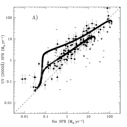
Figure 6: The effect of an enhanced star-formation event on A) the L_Hα – L_UV relation, and B) $UV-B$ versus H$\alpha$ EW. Two example bursts are shown: one involves 10 per cent of the galaxy mass in an exponentially decaying burst of e-folding time 45 Myr, the second 30 per cent mass with a time of 20 Myr, generated using the pegase-ii code, a standard IMF, and solar metallicity. The enhanced star-formation events are able to reproduce the scatter and offsets from constant star-formation scenarios seen in the data.

This explanation is supported by our observations and also predicts trends we should see in our spectral diagnostics indicative of the age of the stellar population. In galaxies which are either at the peak of a starburst or which are undergoing a regular star-forming process (those galaxies in which SFRs derived from L_Hα and L_UV agree well), we would expect small values of the Balmer decrement and high values for the H$\alpha$ EW due to the presence of a young stellar population. For galaxies which are in the later stages of a burst of star-formation, where we have excess in UV/$u$’ SFRs compared to H$\alpha$, we would expect larger Balmer breaks and weaker H$\alpha$ EWs as the burst population ages.

We examine these parameters in Fig. 7, showing the distribution of the Balmer break (D4000) and H$\alpha$ EW values as a function of the position of a galaxy on the H$\alpha$_SFR–UV_SFR diagram. As expected, we see some evidence that those systems with the largest residuals from constant SFR scenarios demonstrate features indicative of older stellar populations (larger values of D4000 and smaller H$\alpha$ EWs).

Figure 7: The distribution of the residuals from the constant SFR line on the H$\alpha$_SFR–UV_SFR plane, as a function of the H$\alpha$ EW (upper) and D4000 (lower) for the FOCA galaxies, shown as solid circles. The horizontal dashed lines show the position of constant star-forming galaxies. Overlaid stars show the evolution of these parameters during example starburst events as in Fig. 6. Again, the starburst events are able to reproduce the scatter and offsets seen.

Irregular SFHs clearly help to explain the discrepancies that we see in the relations exploring the different star-formation diagnostics, in particular the ‘excess’ SFRs derived from UV and $u$’ measures when compared to H$\alpha$, and the luminosity dependence of this result. We investigate this hypothesis more quantitatively in Section 5.

5 Analysis

We have reviewed the qualitative evidence that many of the low to intermediate luminosity galaxies in this data set do not possess simple constant or smoothly declining SFHs. This is an important finding in the context of the interpretation of SFR measures from large galaxy redshift surveys, our primary motivation in this section is to quantitatively confirm our findings. With sample photometry that ranges from 2000 Å to $\sim 7000$ Å (plus spectral coverage at optical wavelengths), we are able to investigate any SFHs that are more consistent with the combined dataset, via a simple $\chi^{2}$ modelling technique. We do this by examining the form of the recent SFH in our galaxies, and then discuss the implications for utilising the different star-formation diagnostics for the galaxy population as a whole.

5.1 Evidence for complex star-formation histories?

For each galaxy we have available the following (dust-corrected) measures: i) The H$\alpha$ luminosity, ii) The UV continuum luminosities at 2000 and 3600 Å, iii) The strength of the Balmer Break, D4000, iv) The H$\alpha$ EW, v) The $UV-B$ and $B-r$’ colours. 81 of our galaxies fit these criteria. The amount of extinction in the models is not left as a free parameter, but is constrained observationally using the H$\alpha$/H$\beta$ Balmer decrement as described earlier. Our goal is to examine the form of the most recent star-formation event for which this is an excellent dataset (however it is not able to provide constraints on the SFH in the distant past). In what follows, we assume a Salpeter IMF with mass limits at 0.1 $\mathrm{M}_{\odot}$ and 100 $\mathrm{M}_{\odot}$, solar metallicity and again utilise the pegase-ii population synthesis code.

We begin by considering two simple SFHs, one representing a constant SFH and the other an exponentially declining SFH according to

$$\mathrm{SFR}(t) = M_{0}\ \ \ (\mathrm{M}_{\odot}\,\mathrm{yr}^{-1})$$ (3)

$$\mathrm{SFR}(t) = \frac{M_{0}}{\tau}\exp(-\frac{t}{\tau})\ \ \ (\mathrm{M}_{\odot}\,\mathrm{yr}^{-1})$$ (4)

In equation (3), $M_{0}$ is the SFR and the stellar mass formed at time $t$ is $M_{0}\times t$; in equation (4), $\tau$ is the time constant of the SFH (in Myr) and $M_{0}$ is the total mass formed at time $t=\infty$ (i.e $\int M_{0}/\tau\exp(-t/\tau)dt=M_{0}$). Small values of $\tau$ (e.g. $\tau<5\,\mathrm{Myr}$) approximate instantaneous bursts, large values approximate continuous SFHs.

We construct a grid of galaxy spectra corresponding to the different SFHs as a function of time, with a range of $\tau$ from 500 to 5000 Myr for the exponential model and models ages of up to 12 Gyr. For each galaxy, we shift the model spectra to the observed redshift, and calculate predictions for each of the observed parameters listed above including nebular emission according to the prescription in pegase-ii. We normalise each model (i.e. adjust $M_{0}$) so that the predicted and observed H$\alpha$ emission are identical. We then calculate a $\chi^{2}$ statistic for each model galaxy by comparing the observed and predicted parameters, and find the combination of parameters which minimise this $\chi^{2}$. The probability of each $\chi^{2}$ is then calculated using the incomplete gamma function for the appropriate number of degrees of freedom in each fit.

The key result is that the ‘best-fits’ for 46/81 (57 per cent) of the galaxies in the constant SFH scenarios and 37/81 (46 per cent) of galaxies in the exponential SFH scenarios are rejected at greater than the nominal 99.9 per cent confidence level – i.e for just under half the sample, the model SEDs provide poor representations of the true physical scenario over the full range of $t$ and $\tau$. The principle indicators of the poor fits are the $u$’/UV luminosities and the H$\alpha$ EWs, sensitive to the ratio of ongoing to past star-formation.

Consequently, for the 46 galaxies which are poorly fit by simple SFHs, we extend these models by relaxing the assumption of ‘smooth’ SFHs and include the possibility of a burst of star-formation superimposed on top of the underlying galaxy SFH, represented by

$$\mathrm{SFR}(t) = \frac{(1-f_{b})M_{0}}{\tau_{g}}\exp(-\frac{t}{\tau_{g}})\ \ \ \mathrm{if}\;t<t_{b}$$

$$\mathrm{SFR}(t) = \frac{(1-f_{b})M_{0}}{\tau_{g}}\exp(-\frac{t}{\tau_{g}})$$ (5)

$$\mbox{}+\frac{f_{b}M_{0}}{\tau_{b}}\exp(-\frac{t_{b}-t}{\tau_{b}})\ \ \ \mathrm{if}\;t>=t_{b}$$

with the starburst commencing at time $t_{b}$ and the total mass formed $M_{0}$, a fraction $f_{b}$ formed during the starburst. We ignore times $t<t_{b}$ (simulated above), and assume $t_{b}=8000\,\mathrm{Myr}$ and $\tau_{g}=3.0\,\mathrm{Gyr}$. The results are not sensitive to the choice of these two parameters which define the underlying SED.

We fit for the combination of parameters which minimise the $\chi^{2}$ as before, with stellar masses estimated by integrating the SFH to the best-fitting $t$. The results of the fits using this framework is quite different – all but 6/46 of the galaxies which were poorly fit by regular SFHs now have acceptable fits. Of these, only 3 have fits which are excluded with a very high level of confidence with the 3 others ‘borderline’ fits. The median best-fitting parameters are given in Table 5. Though these parameters do vary widely when considering any one object, they suggest that the most common starbursts are relatively short duration events, involving around 8 – 10 per cent of the galaxy mass, and that we view these galaxies not at the peak of a particular starburst (where H$\alpha$ and UV derived SFRs will be approximately equal), but instead some way into a burst’s lifetime; it is at these times that the H$\alpha$ and UV or $u$’ luminosities are the most discrepant.

Table 5: The median best-fitting parameters for the form of the bursts of star-formation

Parameter	Median value
$\tau_{b}$	23.1
$t_{b}$	125
$f_{b}$	0.09
LOG $M_{\mathrm{stellar}}$	9.91

Our conclusion from this modelling work is that whilst regular SFHs can provide an adequate explanation for approximately half of the sample, they provide poor representations of the remaining galaxies. By relaxing the assumption of a simple SFH, and instead allowing the recent star-formation in the galaxies to evolve according to a simple burst structure, these inconsistencies appear to be resolved.

5.2 Comparisons with other samples

The finding that the SFHs of a substantial fraction of the galaxies in our dataset appear irregular has important implications for surveys that measure SFRs in galaxies via UV measures, which we discuss in the next section. Prior to that analysis, we first examine the results of this survey with other redshift surveys as a consistency check to confirm that the UV-selected galaxy properties make sense within the broader galaxy population.

Comparison of the results of this survey with other samples of UV-selected galaxies at low-redshift are not yet possible due to the lack of low-redshift UV observations (a situation soon to be rectified via the galex experiment), and $U$-band observations must suffice. However, at higher redshift a comparison is easier as $U$-band fluxes are shifted into optical bandpasses. We compare here with five different samples. The first, at $z\simeq 0.25$ and $z\simeq 0.4$, is the emission-line (H$\alpha$) selected sample of Hippelein et al. (2003). Next are two high-redshift samples of Glazebrook et al. (1999) ($z\sim 1$), who observe H$\alpha$ fluxes for a sample of $I$-band selected CFRS galaxies, and Erb et al. (2003), who select $z\sim 2.2$ galaxies using a photometric colour technique. Finally, we show the two $z\simeq 0$ samples of Bell & Kennicutt (2001) and Buat et al. (2002). For all these samples, we take the published H$\alpha$ and UV-continuum fluxes, correct for dust using the Calzetti et al. (2000) prescription if required, and convert to SFRs using our cosmological model and the pegase-ii conversions as appropriate. The samples are then plotted with the FOCA data in Fig. 8.

Figure 8: A comparison of the FOCA $0<z<0.4$ galaxies (data same as Fig. 5) with those from other samples at varying redshifts: Open circles: $z\simeq 0.25$ and $z\simeq 0.4$; Hippelein et al. (2003), Stars: $z\sim 1$; Glazebrook et al. (1999), Squares: $z\sim 2.2$; Erb et al. (2003), Square crosses: $z\sim 0$; Bell & Kennicutt (2001), Triangular crosses: $z\sim 0$; Buat et al. (2002). The solid line shows the best-fit to the FOCA sample. All data are dust-corrected using the Calzetti et al. (2000) prescription.

In high-luminosity systems ($\mathrm{SFR}\ga 5\,\mathrm{M}_{\odot}\,\mathrm{yr}^{-1}$), the only systems probed by the high-redshift studies, the different samples agree well, with some evidence for higher H$\alpha$-derived SFRs in these systems. Whilst this could be caused by under-estimated dust corrections, our alternative hypothesis of irregular SFHs can also explain the observations: high H$\alpha$ luminosity systems are likely near a peak in SFR, where models predict that H$\alpha$ and UV luminosities are at least equal, or should even show an H$\alpha$ excess (as H$\alpha$ light increases in a new starburst more rapidly than UV light).

Below SFRs of $\sim 5\,\mathrm{M}_{\odot}\,\mathrm{yr}^{-1}$, the properties of the different samples begin to diverge. As noted in Section 4.2, the UV-selected sample shows a general excess in the UV-derived SFRs. However, the two $z\simeq 0$ samples demonstrate SFRs that agree well, while the H$\alpha$-selected sample shows a larger scatter in the derived SFRs, with an H$\alpha$ excess at the faint end. Once again, a systematic under-estimation in the dust extinction corrections can explain the H$\alpha$-excess at the faint end, but this does not explain the UV-excess galaxies. Again, all of the results can be consistently interpreted within a framework of non-regular SFHs coupled with the various survey selection criteria: H$\alpha$-selected galaxies are likely to be located at a phase in their SFH where they are either near a peak of a starburst (in galaxies with varying SFHs) and the H$\alpha$-derived SFR is greater than that from the UV, or the galaxies will have regular SFHs and the H$\alpha$ and UV SFRs agree well. The $z\sim 0$ galaxies, with a general optical selection criteria, are likely to represent star-formation across normal Hubble types and are less likely to possess the irregular SFHs found in the FOCA sample which are selected by their UV light. We examine these ideas further in Section 5.3.

5.3 Implications for measuring cosmic star-formation for flux-limited redshift surveys

The finding that a fraction of the galaxies in our sample do not possess simple SFHs has implications for flux-limited redshift surveys such as this. A galaxy that evolves with an intermittent SFH will clearly brighten and dim over the course of its history. We demonstrate this in Fig. 9, where we show the UV evolution of a typical galaxy in our survey and the input SFR(t) required to produce it, together with the flux limit of the FOCA survey ($m_{\mathrm{uv}}=20.75$ in the AB system). We also plot the flux limit and survey parameters of the $z\simeq 0.25$ and $z\simeq 0.4$ H$\alpha$-selected survey of Hippelein et al. (2003).

The bursts of star-formation brighten the model galaxy above the UV flux limit into the detectable magnitude range. Without this boost, a galaxy would otherwise not be detected in the UV unless located at a low redshift. This bias in itself is not serious – it is one of the goals of this redshift survey to measure an integrated star-formation density, including that fraction of star-formation that occurs in a ‘burst mode’ rather than a ‘continuous mode’. However, a more important bias arises due to the time required for the UV light to die away after a burst has completed, thus leading to higher measured SFRs in the UV or $u$’ than might be obtained via alternative diagnostic measures, and higher measured SFRs than the ‘true’ SFR in the galaxy.

We illustrate this using a model taking into account the flux limit of the FOCA survey and H$\alpha$-selected survey. We model a galaxy’s SFH by superimposing a series of bursts onto an exponentially declining SFH between the ages in the galaxy’s history that correspond to $z=0.5$ and $z=0$ in our cosmological model. The variations $\mathrm{UV}(t)$ and $\mathrm{H}{\alpha}(t)$ are calculated, and using the mapping of $\mathrm{time}\rightarrow z$, the apparent magnitude $m_{\mathrm{uv}}(t)$ can then be computed from the luminosity distance and an appropriate $k$-correction calculated from the synthetic spectrum. From the flux limit of the two surveys, the visibility of the galaxy in each survey can be found.

Figure 9: The visibility in the FOCA UV-selected and Hippelein et al. (2003) emission-line selected surveys of a model galaxy undergoing a series of starbursts between $z=0.5$ and $z=0$. The continuous line denotes the UV luminosity; the dashed line the input SFR (the axes are scaled so that the UV luminosity and input SFR agree according to the conversion values in Table 3). The filled circles show the periods during which a galaxy falls within the selection criteria of a FOCA-like survey, and the two overlaid dotted curves show the magnitude limit of the FOCA survey (upper curve) and the sensitivity limit of the H$\alpha$ survey of Hippelein et al. (2003) (lower curve). The vertical shaded areas at $\simeq 0.25$ and $z\simeq 0.4$ show the redshift sensitivity of Hippelein et al. (2003).

Fig. 9 shows this model. There are points over the model galaxy’s evolution when, although the instantaneous SFR of the galaxy lies below the flux limit of the UV survey – i.e. if this SFR were converted to a UV luminosity using a simple constant-SFH assumption the galaxy would not be detected – the galaxy remains in the UV-selected survey due to the slower decline of the UV light. As expected, at higher redshift a galaxy is preferentially picked out if it is undergoing a burst of star-formation and additionally if the galaxy is near the peak of the particular starburst. At lower redshifts, we are able to view the galaxy at later times into a particular starburst event, and only at the lowest redshifts does the underlying (smoothly declining) galaxy SED come into the FOCA survey.

Figure 10: An example simulation of the galaxies in our survey generated by superimposing starbursts of various masses and durations on a selection of underlying galaxy SFHs. By sampling a galaxy’s history at random redshifts (weighted by the co-moving volume) during which the galaxy’s apparent UV and H$\alpha$ luminosities allow detection in the FOCA survey, distributions in the L_Hα – L_UV plane (panel A from Fig. 5) can be generated and compared to the observations. Simulated galaxies are denoted by small dots, observed galaxies by open circles. The solid line denotes equality of SFRs from Table 3.

The effect of these forms of SFHs on the H$\alpha$–UV plane in a UV-selected survey can be seen in Fig. 10. We run 200 simulations, generating SFHs containing a random number of bursts (from zero to three) of varying mass and duration superimposed on underlying histories with $\tau$ from 0.750 to 6 Gyr between $z=0-0.5$. The H$\alpha$ and UV luminosities at 1 Myr intervals are calculated and given a random error distribution identical to that in the survey. The galaxy is recorded (number-weighted by the co-moving volume) if it meets the selection criteria of the UV survey, and then example survey datasets drawn randomly from these results. The distribution of 18000 simulated galaxies in H$\alpha$–UV space can then be generated. An excellent match between the observed galaxy distribution and the simulated galaxies can be seen.

Estimating how ‘biased’ a determination of the SFR derived from a UV continuum measurement in a particular galaxy is (i.e. how much this measurement is over-estimated due to recent star-formation activity) clearly requires a knowledge of the precise form and age of the particular star-formation events. Though these parameters can, in principle, be estimated using techniques such as those in Section 5.1, this can only be done reliably for a sub-sample of the galaxies – and even then there is a considerable uncertainty in the derived parameters due to the lack of infra-red photometry (particularly the total stellar mass).

Instead, we can estimate the effect of the recent SFH in a purely statistical manner based on the entire sample. We can use the plots of Fig. 5 and the statistical tests performed on them to derive relations between UV or $u$’ luminosities and the instantaneous (H$\alpha$-derived) SFR. By fitting the data across the range of SFRs probed in this study, we find:

$$\log(\mathrm{L}_{\mathrm{UV}}) = 40.03+0.75\log(\mathrm{SFR}_{\mathrm{H}{\alpha}})$$

$$\rightarrow\mathrm{SFR} = (\frac{\mathrm{L}_{\mathrm{UV}}}{1.07\times 10^{40}})^{1.33}\,\,\mathrm{M}_{\odot}\,\mathrm{yr}^{-1}$$ (6)

for the UV luminosities, and

$$\log(\mathrm{L}_{u^{\prime}}) = 39.53+0.74\log(\mathrm{SFR}_{\mathrm{H}{\alpha}})$$

$$\rightarrow\mathrm{SFR} = (\frac{\mathrm{L}_{\mathrm{UV}}}{3.39\times 10^{39}})^{1.35}\,\,\mathrm{M}_{\odot}\,\mathrm{yr}^{-1}$$ (7)

for the $u$’ luminosities, where the luminosities are dust-corrected and measured in $\mathrm{erg}\,\mathrm{s}^{-1}\,\mbox{\AA}^{-1}$. This correction is valid over SFRs of approximately 0.1 to 100 $\mathrm{M}_{\odot}\,\mathrm{yr}^{-1}$ for galaxies in this survey selected at 2000 Å. Whilst similar relational forms likely hold for other redshift surveys, the exact form will depend on the selection criteria and hence the number of galaxies with ‘normal’ SFHs admitted into the survey. Even for other UV-selected surveys, selection at a shorter wavelength will be less affected by the effects of starbursts as the UV light dies away more quickly, whilst longer wavelengths could suffer considerable bias.

Understanding the precise impact of this bias on analyses such as the Madau plot is a complex problem. The corrections given above are only applicable to individual galaxies, not to the integrated luminosity density of the survey as a whole, as the standard luminosity function Schechter (1976) parameters ($\alpha$, $M_{\ast}$/$L_{\ast}$ and $\phi_{\ast}$) will be affected in different ways by correcting for this effect. This correction tends to make the SFR in fainter galaxies lower, and hence the appropriate luminosity function slope will be flatter, or $\alpha$ will become less negative, likely leading to a slight decrease in the calculated integrated star-formation density. The luminosity functions and light densities of this sample will be addressed in a forthcoming paper (Treyer, Sullivan & Ellis, in preparation).

The conclusion from this study is that integrated luminosity densities are a poor guide to the complex physical processes at play in these systems. Star-formation densities derived from these measures need to be carefully calibrated, and the effects of different biases at work more fully understood, before the results of flux-limited surveys can be fairly compared.

6 Conclusions

In this paper, we have presented the results of panoramic wide-field optical imaging of a UV-selected galaxy redshift survey, with the aim of further investigating the nature of star-formation in local $z<0.4$ star-forming and starburst galaxies. We have found the following:

1. New $u^{\prime}Br^{\prime}$ photometry, supplemented by DPOSS data, have allowed us to derive aperture corrections for our H$\alpha$ fluxes, as well as more reliable SEDs for all the sample galaxies. There remains a small fraction ($\leq 8$ per cent) of galaxies exhibiting $UV-B$ colours bluer than most starburst models, whilst possessing colours typical of standard SEDs at longer wavelength.

2. We have investigated the dependence of the H$\alpha$, UV and $u$’ luminosity to SFR conversion factors on the IMF and mass ranges, the stellar metallicity and the time since onset of star formation, assuming constant SFHs. Though varying these parameters can have a large effect on individual conversion values, the effect is smaller when considering ratios of these values (e.g. UV/H$\alpha$).

3. Taking advantage of our new dataset, we update the study of Sullivan et al. (2000) and compare SFRs derived from UV or $u$’ and H$\alpha$ luminosities. Assuming simple SFHs, we show the scatter and non-unity best-fitting slopes observed are unlikely to be primarily generated by varying the above parameters.

4. We show that models including a burst or increased period of star-formation superimposed on an otherwise smooth underlying SFH provide much better fits to the data set of $\sim$50% of the galaxies (H$\alpha$, UV and $u$’ luminosities, Balmer Break, H$\alpha$ EW and colours) than a smooth SFH alone.

5. Such burst modes of star formation lead to an overestimate of SFRs derived from UV luminosities in lower luminosity systems, as UV light from less massive stars will still be present after a burst has died away. We propose a simple statistical correction for UV-selected surveys based on the ‘true’ SFRs as derived from H$\alpha$ luminosities which originate only from the most massive stars.

References

- Afonso et al. (2003) Afonso, J., Hopkins, A., Mobasher, B., & Almeida, C. 2003, in press, ApJ, astro–ph/0307175
- Bell (2002) Bell, E. F. 2002, ApJ, 577, 150
- Bell & Kennicutt (2001) Bell, E. F. & Kennicutt, R. C. 2001, ApJ, 548, 681
- Bertin & Arnouts (1996) Bertin, E. & Arnouts, S. 1996, A&AS, 117, 393
- Blain et al. (1999) Blain, A. W., Smail, I., Ivison, R. J., & Kneib, J. 1999, MNRAS, 302, 632
- Brown et al. (2000) Brown, W. R., Kenyon, S. J., Geller, M. J., & Fabricant, D. G. 2000, ApJ, 540, L83
- Bruzual (1983) Bruzual, A. G. 1983, ApJ, 273, 105
- Buat et al. (2002) Buat, V., Boselli, A., Gavazzi, G., & Bonfanti, C. 2002, A&A, 383, 801
- Calzetti et al. (2000) Calzetti, D., Armus, L., Bohlin, R. C., Kinney, A. L., Koornneef, J., & Storchi-Bergmann, T. 2000, ApJ, 533, 682
- Calzetti et al. (1994) Calzetti, D., Kinney, A. L., & Storchi-Bergmann, T. 1994, ApJ, 429, 582
- Cardelli et al. (1989) Cardelli, J. A., Clayton, G. C., & Mathis, J. S. 1989, ApJ, 345, 245
- Charlot & Longhetti (2001) Charlot, S. . & Longhetti, M. 2001, MNRAS, 323, 887
- Coleman et al. (1980) Coleman, G. D., Wu, C. ., & Weedman, D. W. 1980, ApJS, 43, 393
- Condon (1992) Condon, J. J. 1992, ARA&A, 30, 575
- Connolly et al. (1995) Connolly, A. J., Szalay, A. S., Bershady, M. A., Kinney, A. L., & Calzetti, D. 1995, AJ, 110, 1071
- Connolly et al. (1997) Connolly, A. J., Szalay, A. S., Dickinson, M., Subbarao, M. U., & Brunner, R. J. 1997, ApJ, 486, L11
- Contini et al. (2002) Contini, T., Treyer, M. A., Sullivan, M., & Ellis, R. S. 2002, MNRAS, 330, 75
- Cowie et al. (1999) Cowie, L. L., Songaila, A., & Barger, A. J. 1999, AJ, 118, 603
- Cram et al. (1998) Cram, L., Hopkins, A., Mobasher, B., & Rowan-Robinson, M. 1998, ApJ, 507, 155
- Cuillandre et al. (2000) Cuillandre, J., Luppino, G. A., Starr, B. M., & Isani, S. 2000, Proc. SPIE, 4008, 1010
- Donas et al. (1987) Donas, J., Deharveng, J. M., Laget, M., Milliard, B., & Huguenin, D. 1987, A&A, 180, 12
- Erb et al. (2003) Erb, D. K., Shapley, A. E., Steidel, C. C., Pettini, M., Adelberger, K. L., Hunt, M. P., Moorwood, A. F. M., & Cuby, J. 2003, ApJ, 591, 101
- Fanelli et al. (1988) Fanelli, M. N., O’Connell, R. W., & Thuan, T. X. 1988, ApJ, 334, 665
- Fioc & Rocca-Volmerange (1997) Fioc, M. & Rocca-Volmerange, B. 1997, A&A, 326, 950
- Fioc & Rocca-Volmerange (1999) Fioc, M. & Rocca-Volmerange, B. 1999, in astro-ph, astro–ph/9912179
- Folkes et al. (1999) Folkes, S., et al. 1999, MNRAS, 308, 459
- Fukugita et al. (1995) Fukugita, M., Shimasaku, K., & Ichikawa, T. 1995, PASP, 107, 945
- Gal et al. (????) Gal, R. R., de Carvalho, R. R., Odewahn, S. C., Djorgovski, S. G., Mahabal, A. A., Brunner, R. J., & Lopes, P. A. A. ????, in press, AJ
- Gallagher et al. (1989) Gallagher, J. S., Hunter, D. A., & Bushouse, H. 1989, AJ, 97, 700
- Gallego et al. (1995) Gallego, J., Zamorano, J., Aragon-Salamanca, A., & Rego, M. 1995, ApJ, 455, L1
- Glazebrook et al. (1999) Glazebrook, K., Blake, C., Economou, F., Lilly, S., & Colless, M. 1999, MNRAS, 306, 843
- Haarsma et al. (2000) Haarsma, D. B., Partridge, R. B., Windhorst, R. A., & Richards, E. A. 2000, ApJ, 544, 641
- Heyl et al. (1997) Heyl, J., Colless, M., Ellis, R. S., & Broadhurst, T. 1997, MNRAS, 285, 613
- Hippelein et al. (2003) Hippelein, H., Maier, C., Meisenheimer, K., Wolf, C., Fried, J. W., von Kuhlmann, B., Kümmel, M., Phleps, S., & Röser, H.-J. 2003, A&A, 402, 65
- Hopkins et al. (2001) Hopkins, A. M., Connolly, A. J., Haarsma, D. B., & Cram, L. E. 2001, AJ, 122, 288
- Johnson & Morgan (1953) Johnson, H. L. & Morgan, W. W. 1953, ApJ, 117, 313
- Kennicutt (1983) Kennicutt, R. C. 1983, ApJ, 272, 54
- Kennicutt (1998) —. 1998, ARA&A, 36, 189
- Kewley et al. (2002) Kewley, L. J., Geller, M. J., Jansen, R. A., & Dopita, M. A. 2002, AJ, 124, 3135
- Kron (1980) Kron, R. G. 1980, ApJS, 43, 305
- Kroupa (2001) Kroupa, P. 2001, MNRAS, 322, 231
- Landolt (1992) Landolt, A. U. 1992, AJ, 104, 340
- Lilly et al. (1996) Lilly, S. J., Le Fevre, O., Hammer, F., & Crampton, D. 1996, ApJ, 460, L1
- Madgwick et al. (2002) Madgwick, D. S., et al. 2002, MNRAS, 333, 133
- Mas-Hesse & Kunth (1999) Mas-Hesse, J. M. & Kunth, D. 1999, A&A, 349, 765
- Massey & Gronwall (1990) Massey, P. & Gronwall, C. 1990, ApJ, 358, 344
- Massey et al. (1988) Massey, P., Strobel, K., Barnes, J. V., & Anderson, E. 1988, ApJ, 328, 315
- Milliard et al. (1992) Milliard, B., Donas, J., Laget, M., Armand, C., & Vuillemin, A. 1992, A&A, 257, 24
- Mink (1999) Mink, D. J. 1999, in ASP Conf. Ser. 172: Astronomical Data Analysis Software and Systems VIII, Vol. 8, 498
- Oke (1974) Oke, J. B. 1974, ApJS, 27, 21
- Oke & Gunn (1983) Oke, J. B. & Gunn, J. E. 1983, ApJ, 266, 713
- Poggianti (1997) Poggianti, B. M. 1997, A&AS, 122, 399
- Rowan-Robinson et al. (1997) Rowan-Robinson, M., et al. 1997, MNRAS, 289, 490
- Salpeter (1955) Salpeter, E. E. 1955, ApJ, 121, 161
- Scalo (1998) Scalo, J. 1998, in ASP Conf. Ser. 142: The Stellar Initial Mass Function, ed. G. Gilmore & D.Howell (San Francisco: ASP), 201
- Schechter (1976) Schechter, P. 1976, ApJ, 203, 297
- Schlegel et al. (1998) Schlegel, D. J., Finkbeiner, D. P., & Davis, M. 1998, ApJ, 500, 525
- Searle et al. (1973) Searle, L., Sargent, W. L. W., & Bagnuolo, W. G. 1973, ApJ, 179, 427
- Simcoe et al. (2000) Simcoe, R. A., Metzger, M. R., Small, T. A., & Araya, G. 2000, in American Astronomical Society Meeting, Vol. 196, 5209
- Steidel & Hamilton (1993) Steidel, C. C. & Hamilton, D. 1993, AJ, 105, 2017
- Stone et al. (1999) Stone, R. C., Pier, J. R., & Monet, D. G. 1999, AJ, 118, 2488
- Sullivan (2002) Sullivan, M. 2002, Ph.D. Thesis (Univeristy of Cambridge); abstract appears in The Observatory, 122, 307
- Sullivan et al. (2001) Sullivan, M., Mobasher, B., Chan, B., Cram, L., Ellis, R., Treyer, M., & Hopkins, A. 2001, ApJ, 558, 72
- Sullivan et al. (2000) Sullivan, M., Treyer, M. A., Ellis, R. S., Bridges, T. J., Milliard, B., & Donas, J. . 2000, MNRAS, 312, 442
- Tresse & Maddox (1998) Tresse, L. & Maddox, S. J. 1998, ApJ, 495, 691
- Tresse et al. (2002) Tresse, L., Maddox, S. J., Le Fèvre, O., & Cuby, J.-G. 2002, MNRAS, 337, 369
- Treyer et al. (1998) Treyer, M. A., Ellis, R. S., Milliard, B., Donas, J., & Bridges, T. J. 1998, MNRAS, 300, 303
- Valdes (1998) Valdes, F. G. 1998, in ASP Conf. Ser. 145: Astronomical Data Analysis Software and Systems VII, Vol. 7, 53
- Wilson et al. (2002) Wilson, G., Cowie, L. L., Barger, A. J., & Burke, D. J. 2002, AJ, 124, 1258
- Yoshii & Takahara (1988) Yoshii, Y. & Takahara, F. 1988, ApJ, 326, 1
- Zaritsky et al. (1995) Zaritsky, D., Zabludoff, A. I., & Willick, J. A. 1995, AJ, 110, 1602