Optical Monitoring of the Central Region of the Globular Cluster M15 = NGC 7078: New Variable Stars

Abstract

ABSTRACT

We obtained a series of more than two hundred $R$-band CCD images for the crowded central ($115^{\prime\prime}\times 77^{\prime\prime}$) region of the metal-poor globular cluster M15 with an angular resolution of $0\hbox{$.\!\!^{\prime\prime}$}5-0\hbox{$.\!\!^{\prime\prime}$}9$ in most images. Optimal image subtraction was used to identify variable stars. Brightness variations were found in 83 stars, 55 of which were identified with known cluster variables and the remaining 28 are candidates for new variables. Two of them are most likely SX Phe variables. The variability type of two more stars is uncertain. The remaining stars were tentatively classified as RR Lyrae variables. A preliminary analysis of published data and our results shows that the characteristics of RR Lyrae variables in the densest part ($r<35^{\prime\prime}$) of the cluster probably change. More specifically, the maximum of the period distribution of first- and second-overtone (RR1, RR2) pulsating stars shifts toward shorter periods; i.e., there is an increase in the fraction of stars pulsating with periods $<0\hbox{$.\!\!^{\symoperators d}$}3$ and a deficiency of stars with $0\hbox{$.\!\!^{\symoperators d}$}35\div 0\hbox{$.\!\!^{\symoperators d}$}40$. The ratio of the number of these short-period RR Lyrae variables to the number of fundamental-tone (RR0) pulsating variables changes appreciably. We found and corrected the error of transforming the coordinates of variables V128-155 in M 15 into the coordinate system used in the catalog of variable stars in globular clusters.

1 INTRODUCTION

Globular clusters, particularly their densest central regions, are among the objects whose observational study, as well as the range and level of problems to be solved, significantly depend on the limiting angular resolution achievable in observations. Obviously, new important results of the study of the stellar composition and basic parameters of globular clusters in our Galaxy and others have been obtained from observations that have recently been performed with the Hubble Space Telescope (HST) and ground-based telescopes installed at sites with the best astronomical climate.

The detection and study of photometrically variable objects in crowded stellar fields belong to the range of problems related to the investigation of the stellar populations of globular clusters. Observationally, variable stars of low (compared to RR Lyrae stars) luminosity and small variability amplitude in the central regions of these clusters are the most difficult objects to detect. These primarily include the stars that fall into the region of the so-called blue stragglers in the color-magnitude diagram, as well as the region of the turn-off point and near the main sequence. They are represented by pulsating, eclipsing, and cataclysmic variables. Our primary objective was to attempt to detect such stars, along with hitherto undetected RR Lyrae variables, in the densest central part of the globular cluster M15 where their number can be large, considering the parameters and the stage of dynamical evolution of this cluster.

By its parameters, M15 is, in a sense, a unique object among the Galactic globular clusters, especially among those observable in the Northern Hemisphere. According to the catalog by Harris (1996), M15 is simultaneously among the clusters with the highest mass, central star-crowding level, and density and is at the evolutionary stage of postcore collapse. This is so far the only Galactic globular cluster for which evidence for the presence of a central intermediate-mass black hole has been obtained (Gerssen et al. 2002, 2003). In addition, it is distinguished by a large population (more than 150) of discovered variable stars (Clement et al. 2001), the overwhelming majority of which are RR Lyrae stars. Recently, this population has been supplemented with new low-luminosity variables (Jeon et al. 2001a, 2001b).

In Section 2, we describe the observational data, their reduction, and our method of searching for variables and their photometry. Basic data on the new variable stars are presented and described in Section 3. In Section 4, we make a preliminary comparison of the parameters of the populations of RR Lyrae variables in the central and outer parts of M15.

2 OBSERVATIONS AND THEIR REDUCTION

Our observational data form the basis for solving the problem formulated above. These data aptly combine a high time resolution and a stable subarcsecond angular resolution throughout the two sets (each three hours long) of our optical monitoring of the central region in the globular cluster M15.

2.1 Observational Data and Preliminary Reduction

We carried out our observations with the 1.5-m AZT-22 telescope at the Maidanak Observatory (Mount Maidanak, Uzbekistan) during two consecutive nights, on July 31 and August 1, 2001. The two nights were estimated to be photometric. The detector was an ST7 CCD camera mounted at the short (f/7.7) Ritchey-Chretien focus of the AZT-22 telescope. The CCD array of the camera has $765\times 510$ light-sensitive pixels $9\times 9$ $\mu$m in size, which corresponds to a pixel angular size of $0.15^{\prime\prime}\times 0.15^{\prime\prime}$ and a $115^{\prime\prime}\times 77^{\prime\prime}$ field of view of the camera for this AZT-22 configuration. The observations were performed in a photometric band close to the standard Johnson-Cousins $R$ band in a continuous frame-by-frame imaging mode with an exposure of 1 min per frame. Given the image digitization and recording time, the imaging rate was about 40 frames per hour. The upper culmination of M15 occurred at the middle of each set of observations. The total volume of our observational data for the two nights was 248 frames (below, by the term frame, we mean the two-dimensional array of counts that reproduces the intensity distribution in the recorded image). The seeing estimated for all of our frames from the full width of the seeing image at half maximum (FWHM) showed a subarcsecond resolution almost for the entire volume of our data. The average seeing for the two sets was $0\hbox{$.\!\!^{\prime\prime}$}74$; an appreciable fraction of frames has a seeing FWHM $<0\hbox{$.\!\!^{\prime\prime}$}6$.

The preliminary CCD image reduction included the standard procedures of dark-current subtraction, flat fielding, and cosmic-ray particle hit removal. The mean dark current was estimated by averaging a series of 15 "dark" frames, which gives a dark-current master frame. The normalized master frame of a uniform flat field obtained by the median combination of a series of 15 frames containing the $R$-band images of twilight sky regions was used for the flat fielding. Charged cosmic-ray particle hits in the form of quasi-pointlike peaks were identified in each frame and removed by interpolating the counts in the surrounding pixels. Previously, when studying the photometric properties of the ST7 camera, we found a slight nonlinearity of the output signal (about $10\%$ in the entire range), which probably results from the adjustments of the ST7 output amplifier. Based on tests, we obtained a dependence of the counts in the CCD image on the intensity of the input signal varied in a known way and fitted it by a polynomial. Using this fit, we corrected the intensity in each frame of observational data for nonlinearity.

2.2 The Data-Reduction Technique and Results

The search for and photometry of variable stars in crowded stellar fields are an important but, at the same time, difficult problem, particularly for extremely dense objects like the centers of globular clusters. The conventional approach to this problem realized in the standard software packages for stellar-field photometry (DaoPhot, DoPhot) is based on the point-spread function (PSF) fitting technique and involves the decomposition or modeling of groups of close stars by using a particular PSF representation method followed by the estimation of the coordinates and magnitude for each of the stars in the group. Although most of the stellar-field photometry results obtained to date are based on this approach, we know several difficulties that arise when using the PSFphotometry methods. At a high star density in the image, it becomes difficult both to estimate the underlying sky background level and to properly estimate the parameters of the PSF itself. Therefore, the problem of identifying and photometrically measuring variable sources becomes much more complex.

The above difficulties stimulated the search for alternative approaches to the problem of searching for variable objects in crowded stellar fields. In particular, image-subtraction methods were developed. In general, the input data in the search for variable objects are series of sequential frames that contain the images of objects in a selected region of the sky. The idea of the image-subtraction methods is to obtain information about the brightness behavior of a source by analyzing the difference between the image in each of the frames from the series and the image in a fixed reference frame. The main problem in implementing the image-subtraction methods is the proper reduction of the PSF in the reference frame to the PSF in the current frame. The optimal image-subtraction (OIS) method that has recently been suggested by Alard and Lupton (1998) elegantly solves this problem and allows a nearly optimal difference between the images, i.e., limited by photon noise, to be obtained. The OIS method is based on the following simple assumption: if two images of the stellar field were resampled to a common coordinate system (centered), then the counts in the overwhelming majority of the pixels will be close if the PSFs of the two images are identical. The idea of the method is to determine the convolution kernel Ker(u,v) that reduces the reference image $Im(x,y)$ to the current image $Im(x,y)$ by analyzing the differences between the PSFs, i.e., to minimize the following difference in all pixels:

$$\sum_{x,y}\left([{{R}\otimes{Ker}}](x,y)-Im(x,y)-Bg(x,y)\right)^{2}\rightarrow\min$$ (1)

where x,y are the coordinates in the centered frame, $Bg(x,y)$ specifies the difference between the sky background counts, and the symbol $\otimes$ denotes a discrete convolution. The latter is defined in a pixel with x,y coordinates as

$$\sum_{u=x-p}^{x+p}\sum_{v=y-q}^{y+q}R(u,v)Ker(x-u,y-v)$$ (2)

The convolution kernel Ker(u,v) is specified on a separate [$2\cdot p+1$, $2\cdot q+1$] array. Alard and Lupton (1998) suggested representing Ker(u,v) as a sum of fixed bivariate Gaussian functions (the parameters $\sigma_{k}$) modifed by polynomials with a degree not higher than $i,j$

$$K(u,v)=\sum_{i,j,k,n}A_{n}e^{-\frac{(u^{2}+v^{2})}{2\cdot\sigma_{k}^{2}}}\cdot u^{i}\cdot v^{j}$$ (3)

Representation (3) allows the minimization problem (1) to be linearized with respect to the unknowns $A_{n}$. Thus, the parameters $A_{n}$ of the optimal kernel Ker(u,v) can be determined by solving the system of linear equations by the least squares method. Without dwelling on the detailed description of the method by Alard and Lupton (1998), we note important advantages of the OIS method. When the system of normal equations is constructed, all pixels, i.e., in principle, complete information about the difference between the PSFs of the two images, are used to find the parameters $A_{n}$. The OIS method works more reliably when the star density in the image increases, because more pixels contain information about the PSF difference in denser fields. The intensity-conservation condition can be easily deduced by appropriately normalizing the kernel representation parameters $A_{n}$. Thus, any variations in transparency, exposure time, and the like between the images are automatically eliminated. Finally, the PSF variations over the field can be taken into account in the solution by introducing a dependence of the coefficients $A_{n}$ on the coordinates. In the case of proper subtraction, only the variable part of the intensity remains in the difference image. Thus, only variable objects that are unaffected by the surrounding field can be detected and measured. The difference images can be photometrically measured in a standard way-using aperture or PSF photometry. It should be noted that difference-image photometry gives the variable part of the flux from the object; i.e., when applied to the time sequence of images, it gives a light curve without the constant component. If the total flux is needed for a particular task, then the light curve should be calibrated by performing the photometry of the corresponding objects in the reference image by a standard method. The idea of the OIS method underlies the software that we developed to process the images of M15. The reduction algorithm consisted of the following steps:

(1) Reference-image synthesis. We selected nine frames with the best seeing (FWHM$\sim{0\hbox{$.\!\!^{\prime\prime}$}55\div 0\hbox{$.\!\!^{\prime\prime}$}58}$) from the data of the two sets. Using a system of selected reference stars, we determined the image shifts/rotations in each of the selected frames relative to the coordinate system associated with the CCD array. Subsequently, all of the images were resampled to the same coordinate system by using bivariate spline interpolation and were combined pixel by pixel with median weighting. The resulting reference image has FWHM=$0\hbox{$.\!\!^{\prime\prime}$}56$ and is virtually free from local defects.

(2) Image centering. For the subsequent reduction, all of the images for M15 from the frames of the two observing sets were centered on the reference image. A correlation algorithm was used to determine the shift/rotation parameters. After the interpolation to the coordinate system of the reference image, the new sequence of centered frames was saved as a series of files.

(3) Image subtraction. The main procedure in calculating the difference between the current and reference images involves determining the parameters $A_{n}$ of the optimal convolution kernel (3), which reduces the reference image to the current image. We specified the convolution kernel Ker(u,v) as a sum of three bivariate Gaussian functions with fixed parameters $\sigma_{k}$ 1.3, 2.25, and 3.9 in combination with bivariate modifying polynomials of degrees 4, 3, and 2, respectively. The array size for Ker(u,v) was $31\times 31$ pixels; the difference between the sky background counts $Bg(x,y)$ was specified by a bivariate polynomial of the first degree with appropriate coefficients. In our calculations, we broke down the frames of the reference and current images into nine equal rectangular fragments and determined the parameters $A_{n}$ of the optimal kernel Ker(u,v) in each of these fragments. The coordinate dependence of the PSF may be disregarded within each fragment, which decreases the number of sought-for parameters to 36 and significantly reduces the expenditure of time on the calculations.

Having calculated $A_{n}$ for a given fragment of the current frame, we constructed an optimal kernel Ker(u,v), convolved the corresponding fragment of the reference imagewith this kernel, and subtracted the convolution result from the current fragment. Analysis of the resulting difference image makes it possible to find and fix the coordinates of the pixels that significantly (by more than $3\sigma$) deviate from the mean in a given region of the difference image and that are associated with variable objects or local defects. Using the coordinates of the marked pixels, we eliminated them from the original system of equations and obtained an improved solution by repeating the above procedure of calculating the parameters $A_{n}$.

Having performed the calculations in each of the nine fragments of the current frame, we combined the difference images and formed a full frame of the difference image, which was saved as a file. The absence of any steps at the fragment boundaries in the full difference image is an indicator of proper subtraction.

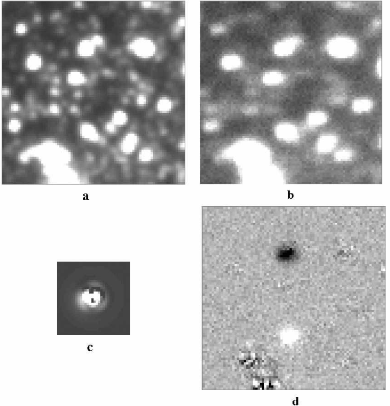
5mm normal

Figure 1: An illustration of how the optimal image-subtraction (OIS) algorithm works. The original fragments of the (a) reference and (b) current images for M15; the fragment size is $12^{\prime\prime}\times 12^{\prime\prime}$; (c) the relative-intensity distribution in the optimal kernel Ker(u,v) calculated from the reference and current images by using the algorithm described in the text. The sizes of the shown image for Ker(u,v) are $31\times 31$ independent pixels; the gradations for the visualization were chosen to optimally reproduce the faint outer wings. The relative-intensity distribution in the image of the optimal convolution kernel reflects the complex PSF shape for the current image (b); (d) the result of the subtraction of the fragment of the reference image (a) convolved with the optimal kernel from the fragment of the current image (b). The gradations were chosen to represent both positive (lighter) and negative (darker) fluctuations of the residual intensity near a zero mean (gray).

Figure 1 illustrates how the described algorithm works. The original fragments of the (Fig. 1a) reference and (Fig. 1b) current images for M15 are shown in the upper part of the figure. Although the PSF in the fragment of the current image (Fig. 1b) is appreciably broader and has a complex elongated shape, the OIS method allows us to find a solution for the optimal convolution kernel Ker(u,v) (Fig. 1c) and perform the subtraction; the corresponding fragment of the difference image is shown in Fig. 1d. The variable stars ZK6 and 7 (the numbers are from our list; the prefix "ZK" means that the star is a candidate for new variables) are clearly identified; we see that in the current fragment, star ZK6 is fainter, while variable 7 is brighter than they are in the reference image. The modulus of the intensity distribution in the difference images of these variables, naturally, corresponds to the PSF of the current image. We also see from Fig. 1d that the subtraction of the surrounding nonvariable stars, including those overlapping with variables ZK6 and 7, was performed properly. The appreciable residual-intensity .uctuations in the difference image (Fig. 1d), which are mainly attributable to photon noise, are observed only at the positions of the brightest stars (see, e.g., to the left and below variable 7).

Having reduced the data from the two sets of observations of M15 using the described algorithm, we obtained the corresponding series of difference image frames for the subsequent analysis. The procedure for finding variable objects can be based both on the analysis of the behavior of each pixel with time, i.e., within the derived sequence, and on the analysis of the average frame from several sequential difference-image frames. We used both approaches to find variable objects. As a result of the selection, we identified a group of pixels with appreciable variability and determined their coordinates (the centroid of the modulus of the difference intensity distribution) in the coordinate system of the reference image. A list of potentially variable objects with the coordinates of their centroids was saved in a separate file for subsequent reduction. The formal measurement error of the centroid coordinates for most objects was about 0.1 pixel ($\sim 0\hbox{$.\!\!^{\prime\prime}$}02$). The ultimate selection of candidates for variable stars was based on photometric data.

We used aperture photometry, which is easier to realize, to measure objects in the difference image. An aperture 10 pixels (1$.\!\!^{\prime\prime}$5) in diameter was used to measure the intensity in the difference image. Based on the centroid coordinates from our list, we measured the intensity of each residual from all of the difference images. Objects with a deviation from the mean of more than 3% within the entire series were classified as candidates for variable stars. Since all of the images, both the original ones before the subtraction and the difference ones, were reduced to the same coordinate system, it will suffice to formally estimate the photometry error from the total-flux fluctuations within the measuring aperture. Placing the measuring aperture in star-centroid coordinates into the frame of the original (before the subtraction) image and summing the intensities, we estimate the rms measurement error $\sigma_{m}$ from the total intensity in the aperture (under the assumption of Poisson statistics):

$$\sigma_{m}=\frac{1}{\sqrt{\sum_{i}{\left(I_{0i}*g\right)}}}$$ (4)

The summation is over the pixels within the aperture (index $i$), $I_{0i}$ is the intensity in pixel $i$ before the subtraction (including the sky background), and $g$ is the number of electrons per ADC unit. Our estimates of the formal error $\sigma_{m}$ vary within the range $0\hbox{$.\!\!^{\symoperators m}$}03-0\hbox{$.\!\!^{\symoperators m}$}005$, depending on the object’s brightness.

Since we have a sample of almost homogeneous measurements at our disposal, we can also directly estimate the photometry error by analyzing the scatter of individual points about the mean (e.g., on monotonic segments of the light curve after the elimination of the trend). The formal and direct estimates of the photometry errors made for several objects are in satisfactory agreement. Therefore, we considered it possible to use the formal estimate for the remaining objects.

Our reduction of the data from the two sets of observations in a $115^{\prime\prime}\times 77^{\prime\prime}$ central region of M15 revealed 83 stars with appreciable variability on short time scales. The coordinates and light curves relative to the reference frame form the basis for the subsequent analysis of our sample of candidates for variable stars.

3 NEW VARIABLE STARS

3.1 The Identification of Variables and the Determination of Their Coordinates

The overwhelming majority of the new variables in the densest central ($r<20^{\prime\prime}$) region of M15 were discovered in the past decade by Ferraro and Paresce (1993) and Butler et al. (1998), who used observations with the HST and the William Herschel (4.2-m) telescope, respectively. A series of several tens of cluster images with a subarcsecond angular resolution allowed the latter authors to confirm the variability of 15 stars from the list by Ferraro and Paresce (1993), to discover 13 new variables (apart from the two known variables V83 and V85), to obtain the phased light curves, and to determine the variability periods for all of these stars. In the catalog by Clement et al. (2001), these 28 new variables are designated as V128-155. However, their coordinates in this catalog proved to be erroneous in the sense that they do not correspond to its coordinate system. This fact was established during the identification by using the cataloged and original data. The formulas in the catalog that were used to recalculate the coordinates are erroneous.

For the above stars, Butler et al. (1998) provided both highly accurate rectangular coordinates (in pixels) and a finding chart. Therefore, we were able to reliably identify 19 of the 28 stars with the corresponding stars from our list: V128-142 (46, 61, 58, 59, 60, 57, 56, 53, 51, 50, 38, 42, 35, 30, 36), V144 (25), V145 (24), V152 (45), V155 (66). The numbers of the variables from our list are given in parentheses. It does not include the nine remaining stars, because they exhibited no light variations in our images. Two more stars (565 and 1417) from the list by Butler et al. (1998), which most likely correspond to V83 and V85, are also reliably identified with stars 21 and 17 from our list, respectively.

Apart from the stars considered above, several dozen of other known variables from the catalog by Clement et al. (2001), which is known to be an extension of the catalog by Sawyer Hogg (1973), fall within our observed field of M15. Unfortunately, the main drawbacks related to the rectangular ($x^{\prime\prime},y^{\prime\prime}$) coordinate system of the catalog by Sawyer Hogg (1973) passed to the catalog by Clement et al. (2001). For well-known reasons, the accuracy of these coordinates in the catalog is low for most of the variable stars. In particular, as Kadla et al. (1988) pointed out, the positions of variables in M15 were determined in two rectangular coordinate systems with a difference between the zero points larger than $2^{\prime\prime}$ along each of the axes back in the first quarter of the past century. Therefore, in some cases, confusion with the identification of variables arises, because the differences between their positions determined by different authors reach several arcseconds. In the absence of finding charts, this circumstance makes it difficult to unambiguously identify new variables with previously discovered ones. This is especially true for the central parts of variable-rich globular clusters, such as M15, where the probability of a close neighborhood of variables is high. We also ran into this problem. However, Kadla et al. (1988) published a finding chart for variable stars in the part of the cluster concerned. Therefore, we were able to solve the problem more or less reliably with a number of controversial cases (see below) that arose when we used the cataloged information about the coordinates of the variables. The authors of the paper mentioned above reduced the coordinates for all of the variables known at that time in M15 to the same coordinate system and pointed out the cases where the same stars were denoted in the catalog by different numbers.

The final identification procedure was performed as follows. We determined the variables from the catalog by Clement et al. (2001) that were most reliably identified with stars from our list (mostly in the outer parts of the observed cluster field) and transformed the coordinate system of the former to the coordinate system of the latter. Subsequently, we determined the equatorial coordinates for the stars from the list by Butler et al. (1998), our list, and the catalog by Clement et al. (2001), naturally, by excluding variables V128-155 from it. In this case, reference stars from the catalog of M15 stars by Yanny et al. (1994) were used for referencing to the equatorial coordinate system. For the stars from all of the lists, we determined the differences $\Delta\alpha$ and $\Delta\delta$ from their equatorial coordinates relative to the M15 center (the position of the object AC 211), whose coordinates, $\alpha_{2000}=21^{h}29^{m}58\hbox{$.\!\!^{\symoperators s}$}26$ and $\delta_{2000}=+12\hbox{${}^{\circ}$}10\hbox{${}^{\prime}$}02\hbox{$.\!\!^{\prime\prime}$}90$, were taken from the same paper. Taking into account the small size of the cluster field under consideration and its relatively small angular distance from the celestial equator, we simultaneously take these differences as the rectangular coordinates ($x^{\prime\prime}$ and $y^{\prime\prime}$) in the system of the catalog by Clement et al. (2001).

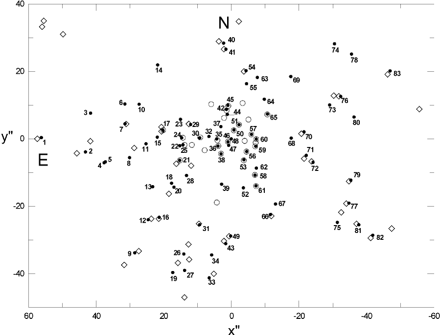
5mm normal

Figure 2: The identification of stars (1-83) from our list (denoted by dots with the corresponding numbers) with known variables. The stars from the catalog by Clement et al. (2001), except V128-155, are indicated by diamonds. The stars from the list by Butler et al. (1998), 28 of which are variables V128-155 and two most likely correspond to V83 and V85, are indicated by circles. The differences $\Delta\alpha^{\prime\prime}$ and $\Delta\delta^{\prime\prime}$ relative to the coordinates of the M15 center are used as $x^{\prime\prime}$ and $y^{\prime\prime}$ of the rectangular coordinate system of the catalog by Clement et al. (2001).

The identification result is shown in Fig. 2. This figure clearly illustrates the above-described reliable and unambiguous identification of a total of 21 stars from our list with the corresponding stars from the list by Butler et al. (1998). The situation with the identification of stars from the catalog by Clement et al. (2001) proved to be less certain and reliable because of several controversial cases. As we see from Fig. 2, each of the stars with numbers 2, 8, 15, 19, 20, 26, 27, 28, 33, 73, and 75 clearly do not coincide with any of the nearby catalogued stars. However, on the finding chart from Kadla et al. (1988) mentioned above, they are identified with the catalogued variables V47, V120, V119, V117, V84, V109, V100, V115, V95, V106, and V107, respectively. For all of the remaining identified stars, the difference between their coordinates ($\Delta x^{\prime\prime}$ and $\Delta y^{\prime\prime}$) and those of the catalogued variables proved to be much smaller and such that $r<2^{\prime\prime}$, where $r=\sqrt{(\Delta x^{\prime\prime})^{2}+(\Delta y^{\prime\prime})^{2}}$. Below, we list the catalogued stars that (apart from the above eleven stars) were identified with stars from our list (their corresponding numbers are given in parentheses): V33 (82), V56 (1), V64 (83), V68-71 (76, 81, 77, 79), V73 (54), V75-77 (43, 49, 66), V79 (16), V81-83 (71, 70, 21), V85-90 (17, 29, 12, 41, 72, 7), and V92-94 (31, 9, 40). In addition, the position of variable 48 in the cluster closely ($<0\hbox{$.\!\!^{\prime\prime}$}1$) matches the position of the well-known object AC 211 (Auriere and Cordoni 1981). Auriere et al. (1984) identified this object with the X-ray source X2127+119 located at the center of M15.

We identified a total of 55 of the 83 stars from our list with known variables, while the remaining 28 stars were classified as candidates for new variables in the globular cluster M15. Their numbers are given in Table 1. This table also presents the coordinates of these stars, which, as was noted above, are the differences $\Delta\alpha^{\prime\prime}$ and $\Delta\delta^{\prime\prime}$ relative to the coordinates of the cluster center in arcseconds. To identify new variables (among all of the 83 stars that we discovered), in describing them in the text, the table, and the figures, we added the prefix "ZK" to their numbers.

Table 2 gives corrected coordinates for V128-155. These coordinates are also the differences $\Delta\alpha^{\prime\prime}$ and $\Delta\delta^{\prime\prime}$, which may be taken with a sufficient accuracy as the rectangular coordinates ($x^{\prime\prime},y^{\prime\prime}$) relative to the cluster center in the system of the catalog by Clement et al. (2001).

3.2 The Classification of New Variables

The basic characteristics of our observations and the achieved accuracy of the (relative) photometry allowed us to reliably establish the fact of light variations in the candidates for variable stars. Unfortunately, however, the total duration of our optical monitoring was not long enough for the same reliable and definite classification of a large number of them. We primarily attribute this to the determination of the subtype of RR Lyrae variables, considering the highest probability of their presence among the discovered new variable stars. At the same time, we do not rule out the erroneous assignment of variables of other types whose periods exceed the duration of each of the two monitoring intervals to the latter. Nevertheless, our quasi-continuous fragments of the light curves make it possible to tentatively estimate the type of the discovered variables from the shape and characteristic features of these curves, the range of brightness variations, etc. This estimate is presented in the column "Type" of Table 1. In addition, this table gives data on the detected brightness variation $\Delta R$, which is not an amplitude value for some of the variables. In designating the different subtypes of RR Lyrae stars, we followed the new system of designations for these subtypes adopted in the catalog by Clement et al. (2001): RR0 corresponds to fundamental-mode pulsations; RR01 corresponds to a double pulsation mode (in the fundamental tone and the first overtone); and RR1 and RR2 correspond to first- and second- overtone pulsations, respectively.

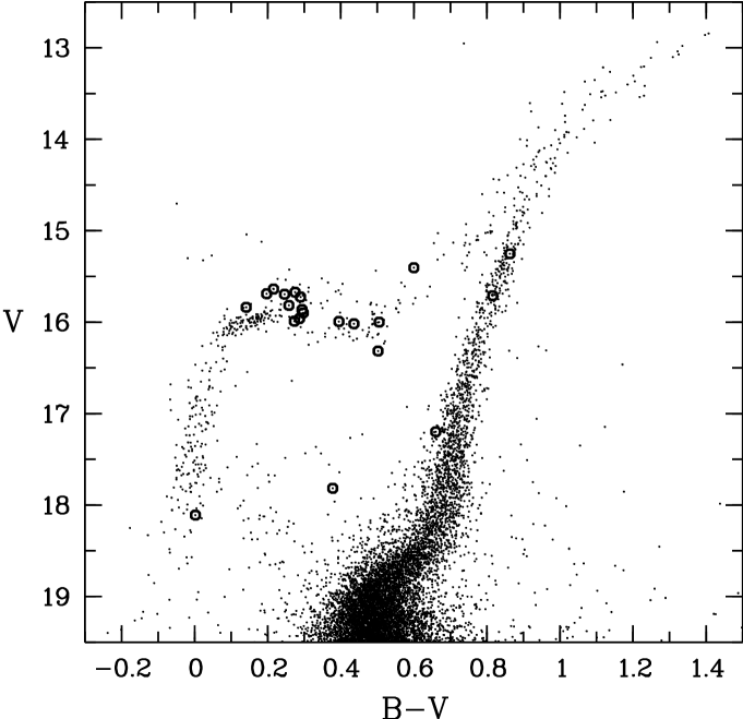
5mm normal

Figure 3: The $V-(B-V)$ diagram for the central region of M15 constructed by using the catalog from van der Marel et al. (2002). The new variables identifid with catalogued stars are indicated by circles.

Although the mean positions of the new variables in the color-magnitude diagram for M15 cannot be determined from our data, we managed to identify most of them with stars in the catalog from van der Marel et al. (2002). It contains photometric data for almost 32 000 stars in the central region of M15 that was observed with the HST. Therefore, we determined the positions of the following identified new variables in the $V-(B-V)$ diagram constructed from the data of this catalog (Fig. 3): ZK3 (21552), ZK4 (20097), ZK5 (20118), ZK6 (11423), ZK10 (11776), ZK11 (24953), ZK13 (26619), ZK14 (13564), ZK18 (25693), ZK22 (1855), ZK23 (505), ZK34 (27077), ZK37 (3393), ZK39 (8568), ZK44 (2997), ZK47 (5768), ZK52 (10356), ZK55 (2321), ZK62 (10041), ZK64 (4894), and ZK68 (10344). The new variables ZK34 (876), ZK37 (793), ZK39 (784), ZK44 (722), ZK47 (699), ZK52 (511), ZK64 (332), ZK67 (267), ZK68 (210), and ZK80 (46) were also identified with stars of the photometric catalog from Yanny et al. (1994), which was compiled from early HST observations. The star numbers from these catalogs are given in parentheses. The identified variables are indicated by circles in Fig. 3. With the exception of five stars (for more detail, see below), the positions of the remaining stars in the diagram are in good agreement with their classification as RR Lyrae variables.

As we see from Table 1, we managed to discover two stars, ZK62 and ZK68, that are, undoubtedly, not RR Lyrae variables. The amplitude and period ($<0\hbox{$.\!\!^{\symoperators d}$}08$) of their brightness variations allow us to classify these stars with a high probability as SX Phe variables, especially since, as we see from Fig. 3, ZK62 and ZK68 fall into the region of blue stragglers. Details on ZK62 and ZK68 will be presented in a separate publication. Note that, currently, only one variable of this type is known in M15. Recently, Jeon et al. (2001a) detected it at a distance of several arcminutes from the cluster center. Thus, given the results of our study, the number of SX Phe stars discovered in the globular cluster M15 reached three. In contrast to ZK62 and ZK68, we failed to determine the variability type of the other two variables, ZK32 and ZK47. As follows from the photometric data of van der Marel et al. (2002), the latter proved to be among the red-giant-branch (RGB) stars above the horizontal branch in the $V-(B-V)$ diagram, while according to the data of Yanny et al. (1994), it is located in the $V-(V-I)$ diagram above (by more than $0\hbox{$.\!\!^{\symoperators m}$}5$) the blue part of the horizontal branch. ZK10 and ZK39 also proved to be among the RGB stars in Fig. 3. However, the latter, according to the data of Yanny et al. (1994), is located near the horizontal branch, while in Fig. 3 it lies below this branch by more than $1\hbox{$.\!\!^{\symoperators m}$}0$. Therefore, it may well be that we identified it erroneously in the catalog by van der Marel et al. (2002), because the difference in coordinates between it and the star identified in the catalog was larger than that for other variables.

Note, in addition, that star 48, i.e., the object AC 211, in our images exhibited complex brightness variations. On the first night of our observations, they appeared periodic, with $\Delta R\approx 0\hbox{$.\!\!^{\symoperators m}$}1$ and a period on the order of $0\hbox{$.\!\!^{\symoperators d}$}1$, while on the second night these variations manifested themselves in the relatively slow brightness increase by $\Delta R\approx 0\hbox{$.\!\!^{\symoperators m}$}2$, only with a hint at faster brightness oscillations (at the photometry error level).

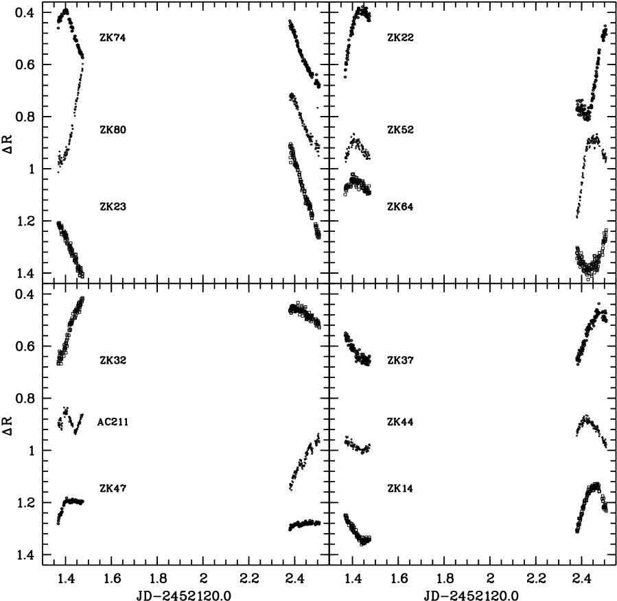
5mm normal

Figure 4: An illustration of the classification by types of new variables based on their light curves. Three light curves for stars of each of the subtypes (a) RR0, (b) RR1, and (d) RR2 are shown as an example. (c) The light curves for the two stars whose variability type could not be determined; also shown here is the light curve for the object AC 211. For convenience, the light curves were arbitrarily displaced along the vertical axis (relative $R$ magnitudes).

Our preliminary classification by types of new variables is illustrated by examples of light curves for twelve of these stars in Fig. 4. Figures 4a, 4b, and 4d show the light curves of RR0, RR1, and RR2 stars, respectively. The light curves of the stars mentioned above whose variability type could not be determined are shown in Fig. 4c. This figure also shows the light curve for the object AC 211. The star numbers are indicated near the corresponding curves. For convenience, we arbitrarily displaced the light curves along the vertical axis ($\Delta R$). Formally, there are no RR01 stars among the candidates for new variables. However, this is not an actual fact. It will be possible to reliably establish whether particular stars are of the RR01 subtype only after the determination of their periods. As we see from the figure, we conditionally classified the stars in which the recorded brightness variation allows the amplitude to be determined and, at the same time, $\Delta R$ is generally within $0\hbox{$.\!\!^{\symoperators m}$}25$ and the shape of the light curve is most likely nearly sinusoidal as being of the RR2 subtype. In this case, there is reason to believe that the second interval of our observations (its duration is $0\hbox{$.\!\!^{\symoperators d}$}128$ compared to the duration $0\hbox{$.\!\!^{\symoperators d}$}107$ of the first interval of our observations) spans about half the pulsation period of the RR2 stars under discussion; i.e., their periods are $<0\hbox{$.\!\!^{\symoperators d}$}3$. The stars classified as RR1 exhibit brightness (including amplitude) variations larger than $0\hbox{$.\!\!^{\symoperators m}$}25$ and an indistinct asymmetry in the light curves. For some of them, the pulsation periods can also be $<0\hbox{$.\!\!^{\symoperators d}$}3$, as those for the stars classified as RR2. The detected brightness variations in RR0 stars proved to be, on average, even larger than those in RR1 stars. In addition, particular characteristic features, such as an asymmetry, a sharp peak, etc., showed up in their light curves. Nevertheless, in several cases, the determination of the subtypes of new variables is controversial or conditional.

4 COMPARATIVE CHARACTERISTICS OF VARIABLE STARS IN THE CENTRAL AND OUTER PARTS OF M15

Almost ten years ago, Stetson (1994) performed multicolor photometry of stars in the central part of M15 by using a large number of CCD images with a subarcsecond angular resolution and an improved procedure of stellar photometry. He found several important changes in the stellar composition that were observed in the cluster region at $r<30^{\prime\prime}$, especially in its densest part ($r<12^{\prime\prime}$), and showed up in the color-magnitude diagram. In particular, these changes manifested themselves in a significant growth of the population of stars that fell into the region in the diagram between the turnoff point and the horizontal branch, as well as in an apparent reddening of the horizontal branch itself. It would be quite natural to assume that the effects resulting in the detected changes in the color-magnitude diagram could also be reflected on the population of variables located in the same part of the cluster and falling into the same region of the diagram. One of the possible changes is quite a natural and expected result of the dynamical effects in the central part of M15 or more specifically, an increase in the number of variables associated with binary stars and blue stragglers. This is confirmed by the study of the central parts of post-core-collapse globular clusters. In particular, in NGC 6397, Kaluzny and Thompson (2002) discovered several variables, among which are eclipsing, cataclysmic, and SX Phe stars. We also managed to discover two SX Phe variables. However, taking into account one of the above results of Stetson (1994), one might expect the actual number of such stars in the central part of M15 to be significant. Whether any changes could affect the population of RR Lyrae variables proper is quite a different matter.

A preliminary (including frequency) analysis of the light curves indicates that there may be a significant fraction of stars with periods $<0\hbox{$.\!\!^{\symoperators d}$}3$ among the new variables classified as RR1 and RR2 and located in the cluster region at $r<35^{\prime\prime}$. The most realistic estimation gives a lower limit on the order of seven (of 15), i.e., more than 40%. We noticed that only five (less than 20%) among the stars of the above subtypes in the catalog by Clement et al. (2001) with measured periods and located at distances $r>35^{\prime\prime}$ from the center of M15 (i.e., with the exception of V128-155, V83, and V85) satisfy this condition; none of them has a period $<0\hbox{$.\!\!^{\symoperators d}$}27$. However, the fraction of such stars (more than 60%) significantly increases among the variables of the above subtypes located in the central region of M15 (i.e., among V128-155, V83, and V85). Almost half of them have periods $<0\hbox{$.\!\!^{\symoperators d}$}27$. The change in the ratio of the numbers of RR Lyrae stars pulsating with periods $<0\hbox{$.\!\!^{\symoperators d}$}3$ and those pulsating in the fundamental tone (RR0) proves to be more significant: 80% in the central region compared to 15% outside it. Yet another significant difference is that only two (of the 25 sample stars) among the variables in the central part of the cluster have periods in the range $0\hbox{$.\!\!^{\symoperators d}$}35\div 0\hbox{$.\!\!^{\symoperators d}$}40$, while there are almost a third of such variables of their total number, more specifically, 24 of the 76 sample stars, in the outer parts of the cluster. A similar change probably also pertains to the numerous population of RR01 stars in the outer parts of the cluster.

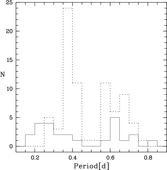
5mm normal

Figure 5: The period distributions (histograms) of RR Lyrae variables in the globular cluster M15. The solid and dotted lines indicate the histograms constructed for stars of the central cluster region ($r<35^{\prime\prime}$) and for the remaining stars, respectively.

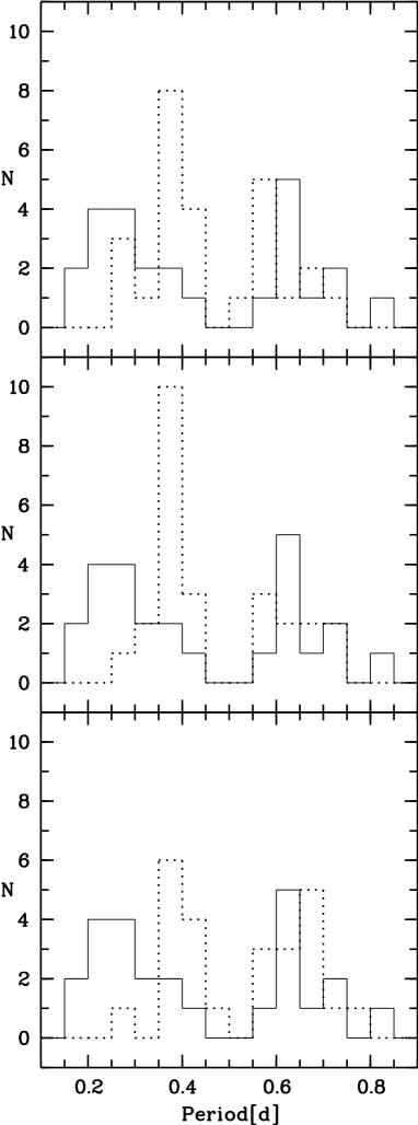
5mm normal

Figure 6: Comparison of the period distributions (histograms, dotted lines) of RR Lyrae variables located in annular zones at difference distances from the center of M15 ($r>175^{\prime\prime}$ (a), $90^{\prime\prime}<r<175^{\prime\prime}$ (b), and $35^{\prime\prime}<r<90^{\prime\prime}$ (c)) with a similar histogram (solid line) constructed for the same variables in the central region ($r<35^{\prime\prime}$) of the cluster. Each zone, except $r>175^{\prime\prime}$ (26 stars), contains 25 stars.

Based on the data from Butler et al. (1998) and from the catalog by Clement et al. (2001) analyzed above, we constructed the histograms (Fig. 5) that clearly show the described differences between the period distributions of the RR Lyrae variables located in different parts of M15. The number of stars in the outer regions of the cluster allows them be separated into three subpopulations (equal in number to the population in the central part) located in annular zones at different distances from the center of M15: 26 stars with $r>175^{\prime\prime}$ and 25 stars each with $90^{\prime\prime}<r<175^{\prime\prime}$ and $35^{\prime\prime}<r<90^{\prime\prime}$. This separation makes it possible not only to analyze the period distributions of variables at different distances from the center of M15 in its outer regions but also to compare each of them with the distribution of stars in the central region. The number of stars in each sample is the same. The derived histograms of the corresponding distributions are represented by dotted lines in Fig. 6 for stars at different distances from the center of M15. As in Fig. 5, the solid line indicates the period distribution of the variables in the central region. We see from a comparison of the histograms that there is no clear evidence of any systematic differences between the period distributions of the RR Lyrae variables in the three outer parts of M15 and that each of them significantly differs from the period distribution in the central part. This suggests that the changes (if they are real) occur almost abruptly somewhere at $r<35^{\prime\prime}$, where the star density significantly increases and where Stetson (1994) found apparent changes in the color-magnitude diagram of the cluster.

Undoubtedly, the size of the sample of variables in the central region of the cluster (25 stars) is much smaller than the size of their sample (76 stars) in the remaining part of M15 and is not yet sufficient to draw ultimate and reliable conclusions. However, the presented differences are too striking to be left unnoticed. In addition, a preliminary analysis of our observations of the new variables reveals the same tendency. Of course, we cannot rule out the possibility that the differences being discussed are attributable to selection effects. One of these effects may stem from the fact that, historically, the variables in the outer parts of M15 were studied mostly by using the methods of photographic photometry of these stars. In contrast, the data on the variables in the central part of the cluster were obtained mainly in the past decade by using much more sophisticated and efficient image recording and reduction techniques. This imbalance between the possibilities of observational studies could lead to the fact that some of the low-amplitude (and, hence, on average, shorter-period) RR Lyrae variables in the outer parts of M15 have proven to be simply undetectable so far. At first glance, this assumption seems quite justified. However, it should be borne in mind that, while studying several tens of known RR Lyrae stars in a wide cluster field using a CCD array, Silbermann and Smith (1995) discovered only one such low-amplitude variable of this type, namely, V113.

With the addition of data on the periods, light curves, and positions in the color-magnitude diagram of our discovered stars and the already known but as yet unstudied variables in the central part of the cluster, the sizes of the samples of variables located in the outer and central regions of M15 will be comparable and quite sufficient for a more substantive analysis.

5 CONCLUSIONS

We carried out two sets of optical monitoring of the central region in the globular cluster M15 with a subarcsecond angular resolution and a total duration of about six hours using the 1.5-m telescope. As a result, we obtained more than two hundred $R$-band images of the cluster. The reduction of our data using the optimal image-subtraction method of Alard and Lupton (1998) revealed brightness variations in 83 stars. Twenty eight of them are candidates for new variables, which constitute the largest population of new variables discovered in one research work in the past 50 years of the study of variable stars in M15. Apart from the two stars whose variability type could not be determined, the other two stars are likely to be SX Phe variables, while the remaining stars were tentatively classified as RR Lyrae variables. Published data on the variables of this type located in the central region of the globular cluster and a preliminary analysis of our results show that in the densest part ($r<35^{\prime\prime}$) of the cluster, the maximum of the period distribution for first- and second-overtone pulsating (RR1 and RR2) stars probably shifts toward shorter periods. In addition to an increase in the fraction of these stars pulsating with periods $<0\hbox{$.\!\!^{\symoperators d}$}3$, there is a deficiency of stars in the range of periods $0\hbox{$.\!\!^{\symoperators d}$}35\div 0\hbox{$.\!\!^{\symoperators d}$}40$ compared to the period distribution for the population of variables in the farther outer parts of M15. The ratio of the number of variables with periods $<0\hbox{$.\!\!^{\symoperators d}$}3$ to the number of variables pulsating in the fundamental tone (RR0) also changes. We found and corrected the error of transforming the coordinates of variables V128-155 to the coordinate system of the catalog by Clement et al. (2001).

Translated by V. Astakhov

0mm flushleft
N $\Delta\alpha^{\prime\prime}$ $\Delta\delta^{\prime\prime}$ $\Delta R$ Type N $\Delta\alpha^{\prime\prime}$ $\Delta\delta^{\prime\prime}$ $\Delta R$ Type ZK3 41.65 7.61 0$.\!\!^{\symoperators m}$20 RR1? ZK39 2.91 -13.46 0$.\!\!^{\symoperators m}$28 RR1? ZK4 37.66 -7.09 0$.\!\!^{\symoperators m}$45 RR1? ZK44 1.21 7.25 0$.\!\!^{\symoperators m}$12 RR2? ZK5 37.26 -6.84 0$.\!\!^{\symoperators m}$40 RR1? ZK47 0.81 -1.94 0$.\!\!^{\symoperators m}$10 $?$ ZK6 31.51 10.34 0$.\!\!^{\symoperators m}$30 RR0? ZK52 -3.54 -14.54 0$.\!\!^{\symoperators m}$32 RR1? ZK10 27.30 10.25 0$.\!\!^{\symoperators m}$12 RR2? ZK55 -4.49 16.33 0$.\!\!^{\symoperators m}$25 RR2? ZK11 25.27 -1.47 0$.\!\!^{\symoperators m}$22 RR1?? ZK62 -7.39 -8.70 0$.\!\!^{\symoperators m}$25 SX Phe ZK13 23.29 -14.21 0$.\!\!^{\symoperators m}$30 RR1? ZK63 -7.68 18.19 0$.\!\!^{\symoperators m}$28 RR1? ZK14 21.82 21.92 0$.\!\!^{\symoperators m}$23 RR2? ZK64 -9.75 11.73 0$.\!\!^{\symoperators m}$35 RR1? ZK18 17.70 -13.16 0$.\!\!^{\symoperators m}$52 RR0? ZK67 -13.04 -19.32 0$.\!\!^{\symoperators m}$30 RR1? ZK22 15.27 -2.06 0$.\!\!^{\symoperators m}$42 RR1? ZK68 -17.70 0.20 0$.\!\!^{\symoperators m}$20 SX Phe ZK23 15.07 5.78 0$.\!\!^{\symoperators m}$52 RR0? ZK69 -17.58 18.47 0$.\!\!^{\symoperators m}$30 RR1? ZK32 6.65 0.70 0$.\!\!^{\symoperators m}$25 $?$ ZK74 -30.51 28.17 0$.\!\!^{\symoperators m}$30 RR0? ZK34 5.85 -34.44 0$.\!\!^{\symoperators m}$30 RR2? ZK78 -35.53 25.13 0$.\!\!^{\symoperators m}$32 RR1 ZK37 3.12 3.63 0$.\!\!^{\symoperators m}$20 RR2? ZK80 -36.27 6.46 0$.\!\!^{\symoperators m}$40 RR0?

Table 1: Data on the 28 new variables in the central region of M15. N are the numbers of the stars from our list classified as candidates for new variables; $\Delta\alpha^{\prime\prime}$ and $\Delta\delta^{\prime\prime}$ are the differences in equatorial coordinates relative to the coordinates of the M15 center (AC 211, epoch 2000.0), which may be taken with a sfficient accuracy as the rectangular ($x^{\prime\prime},y^{\prime\prime}$) coordinates of the system of the catalog by Clement et al. (2001); $\Delta R$ is the maximum recorded $R$-band brightness variation, which is not an amplitude values for some stars; the column "Type" gives a tentative determination of the variability type.

0mm flushleft
N $\Delta\alpha^{\prime\prime}$ $\Delta\delta^{\prime\prime}$ N $\Delta\alpha^{\prime\prime}$ $\Delta\delta^{\prime\prime}$ N $\Delta\alpha^{\prime\prime}$ $\Delta\delta^{\prime\prime}$ 128 1.03 -0.86 138 3.07 -4.12 148 -3.93 -0.62 129 -7.28 -14.02 139 1.43 8.38 149 2.16 6.20 130 -6.95 -10.71 140 4.15 -0.42 150 5.98 10.25 131 -7.05 -2.23 141 9.23 0.41 151 -7.18 -1.15 132 -7.35 -0.09 142 3.86 -2.11 152 0.92 9.77 133 -5.90 1.30 143 4.32 -18.88 153 -5.05 5.71 134 -4.44 -3.79 144 13.89 -1.81 154 -3.32 10.60 135 -3.68 -6.38 145 14.38 0.31 155 -10.64 7.23 136 -2.24 4.20 146 11.69 -1.81 137 -0.71 2.52 147 7.91 -3.38

Table 2: Corrected coordinates of the variable stars V128-155 from the catalog by Clement et al. (2001). N are the numbers of the catalogued stars; $\Delta\alpha^{\prime\prime}$ and $\Delta\delta^{\prime\prime}$ are the same as in Table 1.